DOI: https://doi.org/10.1038/s41598-025-85874-7
PMID: https://pubmed.ncbi.nlm.nih.gov/39794374
تاريخ النشر: 2025-01-10
تقارير علمية
مفتوح
نموذج هجين قابل للتفسير يعتمد على تقنيات التعلم الآلي المتقدمة ونماذج التعلم العميق لتصنيف أورام الدماغ باستخدام صور الرنين المغناطيسي
ملخص
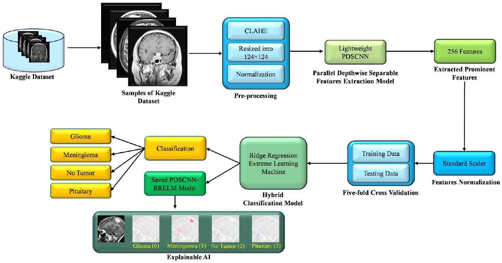
تشكل أورام الدماغ تحديًا صحيًا عالميًا كبيرًا، ويعد الكشف المبكر عنها وتصنيفها بدقة أمرًا حيويًا لاستراتيجيات العلاج الفعالة. تقدم هذه الدراسة نهجًا جديدًا يجمع بين شبكة عصبية تلافيفية قابلة للفصل بعمق خفيف الوزن (PDSCNN) ونموذج هجين من الانحدار الجبهي (RRELM) لتصنيف أربعة أنواع من أورام الدماغ (غليوما، منينجيوما، لا ورم، وغدة نخامية) بناءً على صور الرنين المغناطيسي. يعزز النهج المقترح وضوح وشفافية ميزات الورم في صور الرنين المغناطيسي من خلال استخدام تعديل تباين الهيستوغرام التكيفي المحدود (CLAHE). ثم يتم استخدام PDSCNN خفيف الوزن لاستخراج الأنماط المحددة للورم مع تقليل التعقيد الحسابي. يتم اقتراح نموذج هجين من RRELM، مما يعزز ELM التقليدي لتحسين أداء التصنيف. تم مقارنة الإطار المقترح مع نماذج متطورة مختلفة من حيث دقة التصنيف، ومعلمات النموذج، وأحجام الطبقات. حقق الإطار المقترح دقة متوسطة ملحوظة، واسترجاع، وقيم دقة بلغت 99.35%، 99.30%، و99.22%، على التوالي، من خلال التحقق المتقاطع بخمس طيات. تفوق PDSCNN-RRELM على نموذج آلة التعلم المتطرفة مع المعكوس الزائف (PELM) وأظهر أداءً متفوقًا. أدى إدخال الانحدار الجبهي في إطار ELM إلى تحسينات كبيرة في أداء التصنيف ومعلمات النموذج وأحجام الطبقات مقارنة بتلك الخاصة بالنماذج المتطورة. بالإضافة إلى ذلك، تم إثبات قابلية تفسير الإطار باستخدام تفسيرات شابلي التراكمية (SHAP)، مما يوفر رؤى حول عملية اتخاذ القرار وزيادة الثقة في التشخيصات الواقعية.
- استخدام CLAHE حسّن من وضوح وشفافية ميزات الورم المهمة في صور الرنين المغناطيسي، مما يعزز من مهام التحليل والتصنيف اللاحقة.
- تم اقتراح شبكة عصبية تلافيفية قابلة للفصل بعمق خفيف الوزن (PDSCNN) لاستخراج الميزات ذات الصلة من صور الرنين المغناطيسي المحسنة. يلتقط هذا النموذج الأنماط المحددة للورم بكفاءة مع تقليل التعقيد الحسابي.
- تم اقتراح نموذج هجين من الانحدار الجبهي (RRELM)، الذي يعزز ELM التقليدي من خلال استبدال المعكوس الزائف بالانحدار الجبهي لتحسين أداء التصنيف.
- قامت هذه الدراسة بمقارنة الإطار المقترح مع نماذج متطورة مختلفة (SOTA) بناءً على أداء التصنيف، ومعلمات النموذج، وأحجام الطبقات.
- تم عرض قابلية تفسير الإطار من خلال استخدام SHAP، مما يسمح بفهم أعمق لعملية اتخاذ القرار للنموذج، وزيادة الثقة في تطبيقه التشخيصي في العالم الحقيقي.
مراجعة الأدبيات
أظهر دقة عالية في تصنيف قاعدة البيانات المحدودة من خلال دمج طبقات كثيفة وطبقات إسقاط. تم دمج زيادة البيانات وتطبيع الحد الأدنى والحد الأقصى لتعزيز تباين خلايا الورم. أظهرت النتائج التجريبية أداءً استثنائيًا، مع دقة تدريب تبلغ
وقت الحساب من خلال استغلال القوة التمييزية لشبكة CNN القابلة للفصل بعمق بشكل متوازي. ومن الجدير بالذكر أنه تم تقديم نهج رائد من خلال دمج الانحدار الجبهي في نموذج ELM الهجين المقترح، بدلاً من الطريقة الأكثر زيفًا. يعزز هذا الدمج أداء التصنيف لنموذج الانحدار الجبهي الهجين الجديد (RRELM)، متجاوزًا قدرات الأساليب السابقة. بالإضافة إلى ذلك، تم تجاوز الحدود البحثية التقليدية من خلال تحقيق مستوى غير مسبوق من القابلية للتفسير ضمن الإطار المقترح. من خلال تطوير شبكة CNN-ELM الهجينة القابلة للتفسير، حصل المؤلفون على رؤى حول كيفية عمل النموذج المقترح، مما سمح لهم بفك شفرة المناطق المحددة في الصورة التي تساهم بشكل بارز في تصنيف أورام الدماغ. لقد ظهرت التعلم بالنقل كنهج محوري في تمثيل الصور، لا سيما في المجالات التي تحتوي على بيانات محدودة معلمة. تسلط الدراسة حول التعرف على فئات الطعام Zhang et al.
المنهجية
الإطار المقترح
مجموعة بيانات أورام الدماغ
معالجة البيانات
شبكة عصبية تلافيفية قابلة للفصل بعمق متوازي
الخوارزمية 1
إدخال:
k : عدد النوى المتوازية
س : حجم كل نواة متوازية (مصفوفة بطول k)
c: عدد القنوات
filter_heights: ارتفاع الفلتر لكل نواة متوازية (مصفوفة بطول k)
عرض الفلتر: عرض الفلتر لكل نواة متوازية (مصفوفة بطول k)
الإخراج:
num filters_concat: عدد الفلاتر في الطبقة المدمجة
إجمالي المعلمات: إجمالي عدد المعلمات في الطبقات المتوازية
الإجراء:
- تعيين num_filters_concat
- تعيين total_parameters
- لـ
إلى ك :
أ. تعيين منطقة الفلترارتفاعات_الفلاتر[i] * عرض_الفلاتر[i]
ب. تعيين depthwise_params* filter_heights[i] * filter_widths[i]
ج. تعيين المعلمات نقطة بنقطة
د. إذا كانت عملية الالتفاف قابلة للفصل:
إذا كانت الالتفافات طبيعية:
إضافة p إلى إجمالي المعلمات
4. إرجاع num _filters_concat، total_parameters
التفاعل بين PDSCNN و RRELM
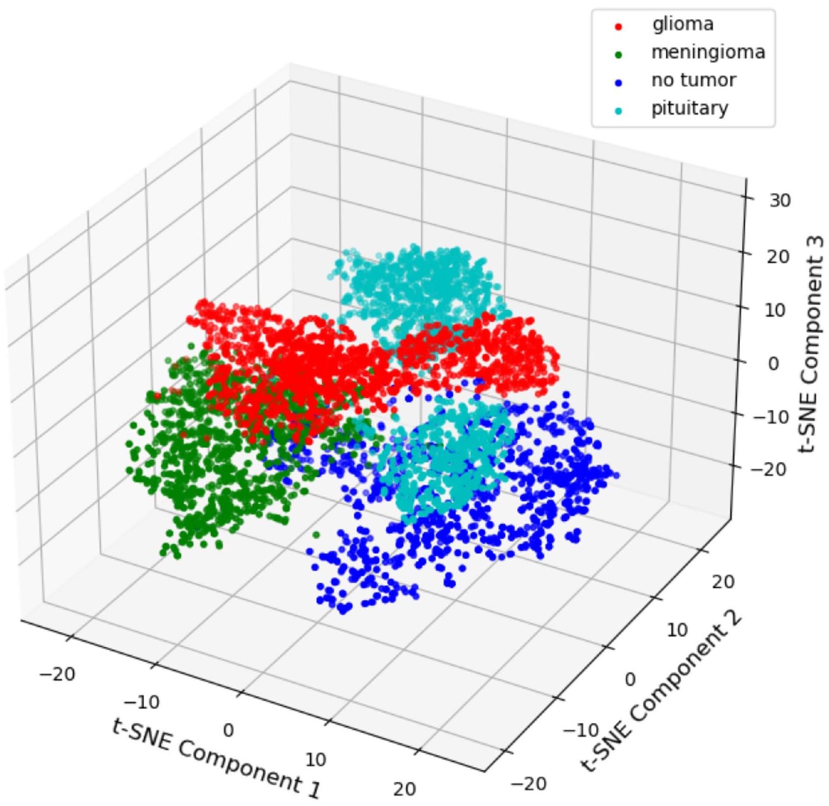
تصوير t-SNE في 3D
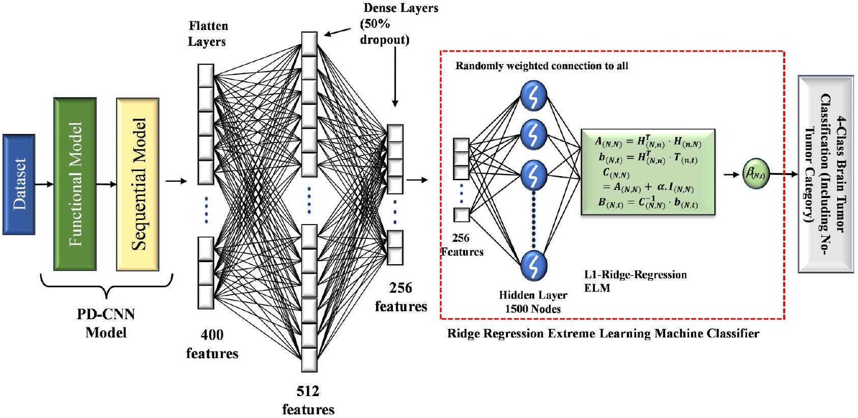
آلة التعلم المتطرفة الانحدار
التهيئة: تم تهيئة مصفوفة أوزان الإدخال (input_weights) بحجم (input_size × hidden_size) والتحيزات بشكل عشوائي باستخدام توزيع طبيعي.
دالة التنشيط: تم استخدام دالة الوحدة الخطية المعدلة (ReLU) كدالة تنشيط للطبقة المخفية. يمكن تعريفها على أنها
حساب الطبقة المخفية: تقوم دالة hidden_nodes() بحساب ناتج الطبقة المخفية (H_train) باستخدام المعادلات التالية.
H_train
output_weights = inv (H_train. T @ H_train + alpha * I) @ H_train. T @ y_train، حيث alpha هو معلمة التنظيم، و I تمثل مصفوفة الهوية بحجم hidden_size، و y_train تشير إلى التسميات المستهدفة.
التنبؤ: تم تقديم دالة predict() لإجراء التنبؤات باستخدام النموذج المدرب. تحسب ناتج الطبقة المخفية للميزات المدخلة المعطاة ( X ) باستخدام المعادلات التالية.
التنبؤات
من خلال دمج الانحدار Ridge ضمن إطار عمل ELM (RRELM)، كانت هذه المنهجية تهدف إلى تحقيق توازن بين تعلم الميزات الفعال والتنظيم، مما يعزز قدرة النموذج على التعميم وإنتاج تنبؤات دقيقة.
مصفوفات التقييم والتنفيذ
النتائج والمناقشة
نموذج ELM مع المعكوس الزائف
ELM مع الانحدار الجبهي
| رقم الطي | اسم الأمراض | دقة | استدعاء | درجة F1 | الدقة (%) |
| طية 1 | ورم دبقي (0) | 0.99 | 0.99 | 0.99 | – |
| ورم السحايا (1) | 0.99 | 0.98 | 0.99 | – | |
| لا ورم (2) | 1.00 | 1.00 | 1.00 | – | |
| الغدة النخامية (3) | 0.99 | 0.99 | 0.99 | – | |
| متوسط | 0.9925* | 0.99 | 0.9925 | 99.21 | |
| فولد 2 | ورم دبقي (0) | 0.99 | 0.99 | 0.99 | – |
| ورم السحايا (1) | 0.98 | 0.99 | 0.98 | – | |
| لا ورم (2) | 1.00 | 1.00 | 1.00 | – | |
| الغدة النخامية (3) | 0.99 | 1.00 | 0.99 | – | |
| متوسط | 0.99 | 0.9950 | 0.99 | 99.21 | |
| فولد 3 | ورم دبقي (0) | 0.99 | 0.99 | 0.99 | – |
| ورم السحايا (1) | 0.98 | 0.98 | 0.98 | – | |
| لا ورم (2) | 1.00 | 1.00 | 1.00 | – | |
| الغدة النخامية (3) | 1.00 | 0.99 | 1.00 | – | |
| متوسط | 0.9925 | 0.99 | 0.9925 | 99.14 | |
| فولد 4 | ورم دبقي (0) | 0.98 | 0.98 | 0.98 | – |
| ورم السحايا (1) | 0.99 | 0.98 | 0.98 | – | |
| لا ورم (2) | 1.00 | 1.00 | 1.00 | – | |
| الغدة النخامية (3) | 0.99 | 1.00 | 0.99 | – | |
| متوسط | 0.99 | 0.99 | 0.9875 | 99.00 | |
| فولد 5 | ورم دبقي (0) | 1.00 | 0.98 | 0.99 | – |
| ورم السحايا (1) | 0.97 | 0.99 | 0.98 | – | |
| لا ورم (2) | 1.00 | 1.00 | 1.00 | – | |
| الغدة النخامية (3) | 0.99 | 0.99 | 0.99 | – | |
| متوسط | 0.99 | 0.99 | 0.99 | 99.07 |
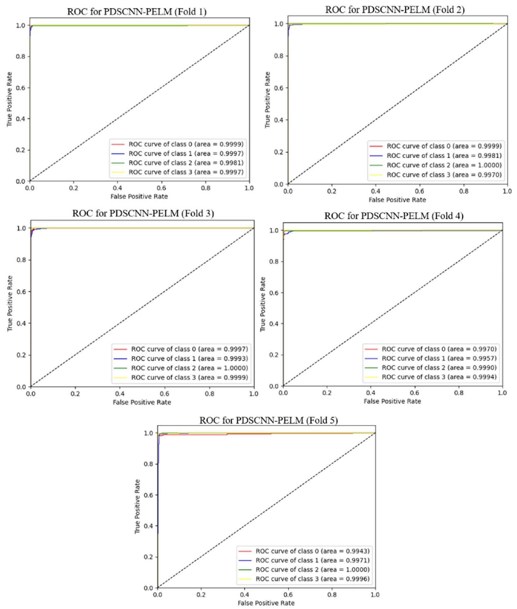
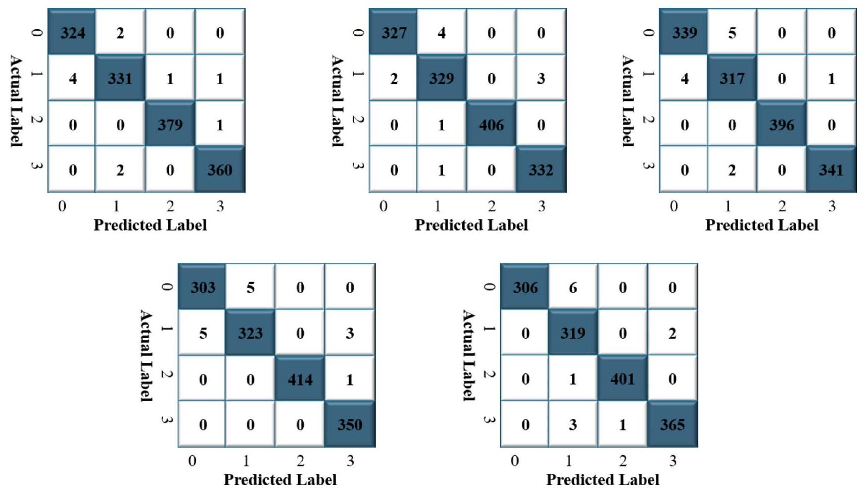
مقارنة بين PELM و RRELM
| رقم الطي | اسم الأمراض | دقة | استدعاء | درجة F1 | الدقة (%) |
| طية 1 | ورم دبقي (0) | 0.99 | 1.00 | 0.99 | – |
| ورم السحايا (1) | 0.99 | 0.98 | 0.98 | – | |
| لا ورم (2) | 1.00 | 1.00 | 1.00 | – | |
| الغدة النخامية (3) | 0.99 | 0.99 | 0.99 | – | |
| متوسط | 0.9925 | 0.9925 | 0.99 | 99.28 | |
| فولد 2 | ورم دبقي (0) | 1.00 | 0.98 | 0.99 | – |
| ورم السحايا (1) | 0.98 | 0.99 | 0.98 | – | |
| لا ورم (2) | 1.00 | 1.00 | 1.00 | – | |
| الغدة النخامية (3) | 0.99 | 0.99 | 0.99 | – | |
| متوسط | 0.9925 | 0.99 | 0.99 | 99.14 | |
| فولد 3 | ورم دبقي (0) | 0.99 | 0.99 | 0.99 | – |
| ورم السحايا (1) | 0.99 | 0.98 | 0.98 | – | |
| لا ورم (2) | 1.00 | 0.99 | 1.00 | – | |
| الغدة النخامية (3) | 0.99 | 1.00 | 0.99 | – | |
| متوسط | 0.9925 | 0.9925 | 0.99 | 99.04 | |
| فولد 4 | ورم دبقي (0) | 1.00 | 0.99 | 0.99 | – |
| ورم السحايا (1) | 0.99 | 0.99 | 0.98 | – | |
| لا ورم (2) | 1.00 | 1.00 | 1.00 | – | |
| الغدة النخامية (3) | 0.99 | 1.00 | 1.00 | – | |
| متوسط | 1.00* | 1.00 | 1.00 | 99.50 | |
| فولد 5 | ورم دبقي (0) | 0.99 | 0.98 | 0.99 | – |
| ورم السحايا (1) | 0.97 | 0.99 | 0.98 | – | |
| لا ورم (2) | 1.00 | 1.00 | 1.00 | – | |
| الغدة النخامية (3) | 1.00 | 1.00 | 1.00 | – | |
| متوسط | 0.99 | 0.9925 | 0.9925 | 99.14 |
| اسم الطراز | متوسط الدقة
|
استرجاع
|
درجة F1
|
دقة
|
الجامعة الأمريكية في القاهرة
|
| PDSCNN-PELM |
|
|
|
|
|
| PDSCNN-RRELM |
|
|
|
|
|
مقارنة أداء PDSCNN-RRELM مع نماذج SOTA
قابلية تفسير PDSCNN-RRELM باستخدام SHAP
| مرجع | حجم مجموعة البيانات | فئة الهدف | الدقة (%) | استرجاع (%) | درجة F1 (%) | الدقة (%) | العائد السنوي المركب (%) | المعلمات (مليون) | طبقات | نموذج |
| جومعي وآخرون
|
قطار: 2145 اختبار: 919 | ٣ | – | – | – | ٩٤.٢٣٣ | – | – | – | ريلم |
| مزوقي وآخرون
|
قطار: 284 اختبار: 67 | 2 | – | – | – | ٩٦.٤٩ | – | – | – | شبكة عصبية تلافيفية ثلاثية الأبعاد |
| خان وآخرون
|
التدريب: 2840 الاختبار: 424 | ٣ | 99.13 | – | – | 99.13 | – | – | – | HDL2BT |
| أحمد وآخرون
|
التدريب: 2968 الاختبار: 394 القيمة: 32 | ٤ | – | ٩٦.٣٤ | ٩٨.٢٢ | ٩٧.٩٨ | – | 14 | شبكة عصبية تلافيفية مخصصة | |
| ناياك وآخرون
|
التدريب: 2608 الاختبار: 652 | ٣ | ٩٨.٧٥ | ٩٨.٧٥ | ٩٨.٧٥ | ٩٨.٧٨ | – | 5.3 | ٢٣٠ | نسخة من EfficientNet |
| العنزي وآخرون
|
القطار: 1980 الاختبار: 495 | ٣ | – | – | – | ٩٦.٨٩ | – | – | ٢٢ | نقل التعلم العميق |
| بادزا وآخرون
|
التدريب: 2758 الاختبار: 306 | ٣ | ٩٧.١٥ | 97.82 | ٩٧.٤٧ | ٩٧.٢٨ | – | – | ٢٢ | شبكة عصبية تلافيفية مخصصة |
| ديباك وآخرون
|
قطار: 2450 اختبار: 614 | ٣ | ٩٧.٣٠ | ٩٧.٦٠ | ٩٧.٠٠ | 97.10 | 99.70 | 6.6 | ٢٢ | التعلم العميق للنقل |
| شيك وآخرون
|
التدريب: 2450 الاختبار: 614 | ٣ | ٩٦.١٤ | 95.99 | ٩٦.٠٣ | ٩٦.٥١ | 99.00 | ٢.٤ | 53 | مانيت |
| فردوس وآخرون
|
التدريب: 5156 الاختبار: 1031 | ٣ | – | – | – | ٩٨.١١ | – | ٨ | 14 | LCDEiT |
| ريدي وآخرون
|
التدريب: 5712 الاختبار: 1311 | ٤ | 98.6 | 98.6 | 98.6 | 98.7 | – | – | 32 | FTVT-b32 |
| وانغ وآخرون
|
تدريب: 5800 اختبار: 1400 | ٤ | ٩٨.٨٧ | ٩٨.٤٦ | ٩٨.٦٦ | 98.86 | – | – | 12 | رانمير-فورمر |
| العمل المقترح | قطار:5619 اختبار:1404 | ٤ | 99.35* | 99.30 | 99.25 | 99.22 | 99.99 | 0.53 | 10 | PDSCNN-RRELM |
نُشر على الإنترنت: 10 يناير 2025
References
- Louis, D. N. et al. The 2016 World Health Organization classification of tumors of the central nervous system: A summary. Acta Neuropathol. 131, 803-820 (2016).
- Chahal, P. K., Pandey, S. & Goel, S. A survey on brain tumor detection techniques for MR images. Multimed. Tools Appl. 79, 21771-21814 (2020).
- Guan, Y. et al. A framework for efficient brain tumor classification using MRI images (2021).
- Komninos, J. et al. Tumors metastatic to the pituitary gland: Case report and literature review. J. Clin. Endocrinol. Metab. 89, 574-580 (2004).
- Ahamed, M. F. et al. A review on brain tumor segmentation based on deep learning methods with federated learning techniques. Comput. Med. Imaging Graph. 110, 102313 (2023).
- Faysal Ahamed, M., Robiul Islam, M., Hossain, T., Syfullah, K. & Sarkar, O. Classification and segmentation on multi-regional brain tumors using volumetric images of MRI with customized 3D U-Net framework. In Proceedings of International Conference on Information and Communication Technology for Development: ICICTD 2022 223-234 (Springer, 2023).
- Titu, M. M. T., Mary, M. M., Ahamed, M. F., Oishee, T. M. & Hasan, M. M. Utilizing customized 3D U-Net framework for the classification and segmentation of multi-regional brain tumors in volumetric MRI images. In 2024 3rd International Conference on Advancement in Electrical and Electronic Engineering (ICAEEE) 1-6 (IEEE, 2024).
- Ahamed, M. F. et al. Automated detection of colorectal polyp utilizing deep learning methods with explainable AI. IEEE Access (2024).
- Varuna Shree, N. & Kumar, T. N. R. Identification and classification of brain tumor MRI images with feature extraction using DWT and probabilistic neural network. Brain Inf. 5, 23-30 (2018).
- Nahiduzzaman, M., Islam, M. R. & Hassan, R. ChestX-Ray6: Prediction of multiple diseases including COVID-19 from chest X-ray images using convolutional neural network. Expert Syst. Appl. 211, 118576 (2023).
- Islam, M. R. & Nahiduzzaman, M. Complex features extraction with deep learning model for the detection of COVID19 from CT scan images using ensemble based machine learning approach. Expert Syst. Appl. 195, 116554 (2022).
- Nahiduzzaman, M. et al. Diabetic retinopathy identification using parallel convolutional neural network based feature extractor and ELM classifier. Expert Syst. Appl. 217, 119557 (2023).
- Nahiduzzaman, M. et al. Hybrid CNN-SVD based prominent feature extraction and selection for grading diabetic retinopathy using extreme learning machine algorithm. IEEE Access 9, 152261-152274 (2021).
- Nahiduzzaman, M. et al. A novel method for multivariant pneumonia classification based on hybrid CNN-PCA based feature extraction using extreme learning machine with CXR images. IEEE Access 9, 147512-147526 (2021).
- Hossain, M. M., Islam, M. R., Ahamed, M. F., Ahsan, M. & Haider J. A collaborative federated learning framework for lung and colon cancer classifications. Technologies 12, 151 (2024).
- Hossain, M. M., Ahamed, M. F., Islam, M. R. & Imam, M. D. R. Privacy preserving federated learning for lung cancer classification. In 2023 26th International Conference on Computer and Information Technology (ICCIT) 1-6 (IEEE, 2023).
- Ahamed, M. F., Nahiduzzaman, M., Ayari, M. A., Khandakar, A. & Islam, S. M. R. Malaria parasite classification from RBC smears using lightweight parallel depthwise separable CNN and ridge regression ELM by integrating SHAP techniques (2023).
- Sarkar, O. et al. Multi-scale CNN: An explainable AI-integrated unique deep learning framework for lung-affected disease classification. Technologies 11, 134 (2023).
- Ullah, F., Nadeem, M. & Abrar, M. Revolutionizing brain tumor segmentation in MRI with dynamic fusion of handcrafted features and global pathway-based deep learning. KSII Trans. Internet Inform. Syst. 18 (2024).
- Anwar, R. W., Abrar, M. & Ullah, F. Transfer learning in brain tumor classification: Challenges, opportunities, and future prospects. In 2023 14th International Conference on Information and Communication Technology Convergence (ICTC) 24-29 (IEEE, 2023).
- Akbar, M. et al. An effective deep learning approach for the classification of Bacteriosis in peach leave. Front. Plant Sci. 13. https:/ /doi.org/10.3389/fpls.2022.1064854 (2022).
- Nazar, U. et al. Review of automated computerized methods for brain tumor segmentation and classification. Curr. Med. Imaging 16, 823-834 (2020).
- Ahamed, M. F., Sarkar, O. & Matin, A. Instance segmentation of visible cloud images based on mask R-CNN applying transfer learning approach. In 2020 2nd International Conference on Advanced Information and Communication Technology (ICAICT) 257-262 (IEEE, 2020). https://doi.org/10.1109/ICAICT51780.2020.9333531.
- Musallam, A. S., Sherif, A. S. & Hussein, M. K. A new convolutional neural network architecture for automatic detection of brain tumors in magnetic resonance imaging images. IEEE Access 10, 2775-2782 (2022).
- Simonyan, K. & Zisserman, A. Very deep convolutional networks for large-scale image recognition. arXiv preprint arXiv:1409.1556 (2014).
- Nayak, D. R., Padhy, N., Mallick, P. K., Zymbler, M. & Kumar, S. Brain tumor classification using dense efficient-net. Axioms 11, 34 (2022).
- Alanazi, M. F. et al. Brain tumor/mass classification framework using magnetic-resonance-imaging-based isolated and developed transfer deep-learning model. Sensors 22, 372 (2022).
- Khan, A. H. et al. Intelligent model for brain tumor identification using deep learning. Appl. Computat. Intell. Soft Comput. 2022, 8104054 (2022).
- Irmak, E. Multi-classification of brain tumor MRI images using deep convolutional neural network with fully optimized framework. Iran. J. Sci. Technol. Trans. Electr. Eng. 45, 1015-1036 (2021).
- Badža, M. M. & Barjaktarović, M. Č. Classification of brain tumors from MRI images using a convolutional neural network. Appl. Sci. 10, 1999 (2020).
- Mzoughi, H. et al. Deep multi-scale 3D convolutional neural network (CNN) for MRI gliomas brain tumor classification. J. Digit. Imaging 33, 903-915 (2020).
- Gumaei, A., Hassan, M. M., Hassan, M. R., Alelaiwi, A. & Fortino, G. A hybrid feature extraction method with regularized extreme learning machine for brain tumor classification. IEEE Access 7, 36266-36273 (2019).
- Deepak, S. & Ameer, P. M. Brain tumor classification using deep CNN features via transfer learning. Comput. Biol. Med. 111, 103345 (2019).
- Shaik, N. S. & Cherukuri, T. K. Multi-level attention network: Application to brain tumor classification. Signal. Image Video Process. 16, 817-824 (2022).
- Ahuja, S., Panigrahi, B. K. & Gandhi, T. K. Enhanced performance of Dark-nets for brain tumor classification and segmentation using colormap-based superpixel techniques. Mach. Learn. Appl. 7, 100212 (2022).
- Brain Tumor MRI Dataset. https://www.kaggle.com/datasets/masoudnickparvar/brain-tumor-mri-dataset/data.
- Pisano, E. D. et al. Contrast limited adaptive histogram equalization image processing to improve the detection of simulated spiculations in dense mammograms. J. Digit. Imaging 11, 193-200 (1998).
- Ahamed, M. F., Salam, A., Nahiduzzaman, M., Abdullah-Al-Wadud, M. & Islam, S. M. R. streamlining plant disease diagnosis with convolutional neural networks and edge devices. Neural Comput. Appl. 36, 18445-18477 (2024).
- Ahamed, M. F. et al. Detection of various gastrointestinal tract diseases through a deep learning method with ensemble ELM and explainable AI. Expert Syst. Appl. 256, 124908 (2024).
- Ahamed, M. F. et al. Interpretable deep learning model for tuberculosis detection using X-ray images. In Surveillance, Prevention, and Control of Infectious Diseases: An AI Perspective (eds. Chowdhury, M. E. H. & Kiranyaz, S.) 169-192 (Springer, 2024).
- Huang, G. B., Zhu, Q. Y. & Siew, C. K. Extreme learning machine: Theory and applications. Neurocomputing 70, 489-501 (2006).
- Nahiduzzaman, M. et al. Parallel CNN-ELM: A multiclass classification of chest X-ray images to identify seventeen lung diseases including COVID-19. Expert Syst. Appl. 229, 120528 (2023).
- Nahiduzzaman, M., Nayeem, M. J., Ahmed, M. T. & Zaman, M. S. U. Prediction of heart disease using multi-layer perceptron neural network and support vector machine. In 2019 4th International Conference on Electrical Information and Communication Technology (EICT) 1-6 (IEEE, 2019).
- Kibria, H. B., Nahiduzzaman, M., Goni, M. O. F., Ahsan, M. & Haider, J. An ensemble approach for the prediction of diabetes mellitus using a soft voting classifier with an explainable AI. Sensors 22, 7268 (2022).
- Powers, D. M. W. Evaluation: From precision, recall and F-measure to ROC, informedness, markedness and correlation. arXiv preprint arXiv:2010.16061(2020).
- Swets, J. A. Measuring the accuracy of diagnostic systems. Science (1979) 240, 1285-1293 (1988).
- Ferdous, G. J., Sathi, K. A., Hossain, M. A., Hoque, M. M. & Dewan, M. A. A. LCDEiT: A linear complexity data-efficient image transformer for MRI brain tumor classification. IEEE Access 11, 20337-20350 (2023).
- Reddy, C. K. K. et al. A fine-tuned vision transformer based enhanced multi-class brain tumor classification using MRI scan imagery. Front. Oncol. 141-23 (2024).
- Wang, J., Lu, S. Y., Wang, S. H. & Zhang, Y. D. RanMerFormer: Randomized vision transformer with token merging for brain tumor classification. Neurocomputing 573, 127216 (2024).
- Lundberg, S. A unified approach to interpreting model predictions. arXiv Preprint arXiv:1705.07874 (2017).
- Bhandari, M., Shahi, T. B., Siku, B. & Neupane, A. Explanatory classification of CXR images into COVID-19, Pneumonia and Tuberculosis using deep learning and XAI. Comput. Biol. Med. 150, 106156 (2022).
- Ullah, F. et al. Evolutionary model for brain cancer-grading and classification. IEEE Access 11, 126182-126194 (2023).
- Ullah, F. et al. Enhancing brain tumor segmentation accuracy through scalable federated learning with advanced data privacy and security measures. Mathematics 11, 4189 (2023).
- Ullah, F. et al. Brain tumor segmentation from MRI images using handcrafted convolutional neural network. Diagnostics 13, 2650 (2023).
- Zhang, Y. et al. Deep learning in food category recognition. Inf. Fusion 98, 101859 (2023).
- Lu, S. Y., Nayak, D. R., Wang, S. H. & Zhang Y.-D. A cerebral microbleed diagnosis method via FeatureNet and ensembled randomized neural networks. Appl. Soft Comput. 109, 107567 (2021).
- Lu, S. Y., Zhu, Z., Tang, Y., Zhang, X. & Liu, X. CTBViT: A novel ViT for tuberculosis classification with efficient block and randomized classifier. Biomed. Signal. Process. Control 100, 106981 (2025).
مساهمات المؤلفين
الإعلانات
المصالح المتنافسة
معلومات إضافية
معلومات إعادة الطباعة والتصاريح متاحة علىwww.nature.com/reprints.
ملاحظة الناشر: تظل شركة سبرينجر ناتشر محايدة فيما يتعلق بالمطالبات القضائية في الخرائط المنشورة والانتماءات المؤسسية.
© المؤلفون 2025، نشر مصحح 2025
قسم الهندسة الكهربائية وهندسة الحاسوب، جامعة راجشاهي للهندسة والتكنولوجيا، راجشاهي 6204، بنغلاديش. قسم هندسة تكنولوجيا الفضاء، كلية الهندسة الكهربائية التقنية، الجامعة التقنية الوسطى، بغداد، العراق. قسم علوم الحاسوب، جامعة جيهان السليمانية، السليمانية 46001، إقليم كردستان، العراق. قسم الهندسة الكهربائية، جامعة قطر، الدوحة 2713، قطر. قسم الهندسة المدنية والبيئية، جامعة قطر، الدوحة 2713، قطر. قسم علوم الحاسوب، جامعة يورك، طريق ديرامور، يورك YO10 5GH، المملكة المتحدة. قسم الهندسة، جامعة مانشستر متروبوليتان، شارع تشيستر، مانشستر M1 5GD، المملكة المتحدة. الذكاء الاصطناعي والصحة الرقمية، كلية علوم الصحة وإعادة التأهيل، كلية الصحة والعلوم السلوكية، جامعة كوينزلاند، سانت لوسيا، كوينزلاند 4072، أستراليا. معهد الإلكترونيات الضوئية، الجامعة العسكرية للتكنولوجيا، الجنرال س. كاليكسيغو 2، وارسو 00-908، بولندا. البريد الإلكتروني: marcin.kowalski@wat.edu.pl
DOI: https://doi.org/10.1038/s41598-025-85874-7
PMID: https://pubmed.ncbi.nlm.nih.gov/39794374
Publication Date: 2025-01-10
scientific reports
OPEN
A hybrid explainable model based on advanced machine learning and deep learning models for classifying brain tumors using MRI images
Abstract
Brain tumors present a significant global health challenge, and their early detection and accurate classification are crucial for effective treatment strategies. This study presents a novel approach combining a lightweight parallel depthwise separable convolutional neural network (PDSCNN) and a hybrid ridge regression extreme learning machine (RRELM) for accurately classifying four types of brain tumors (glioma, meningioma, no tumor, and pituitary) based on MRI images. The proposed approach enhances the visibility and clarity of tumor features in MRI images by employing contrastlimited adaptive histogram equalization (CLAHE). A lightweight PDSCNN is then employed to extract relevant tumor-specific patterns while minimizing computational complexity. A hybrid RRELM model is proposed, enhancing the traditional ELM for improved classification performance. The proposed framework is compared with various state-of-the-art models in terms of classification accuracy, model parameters, and layer sizes. The proposed framework achieved remarkable average precision, recall, and accuracy values of 99.35%, 99.30%, and 99.22%, respectively, through five-fold cross-validation. The PDSCNN-RRELM outperformed the extreme learning machine model with pseudoinverse (PELM) and exhibited superior performance. The introduction of ridge regression in the ELM framework led to significant enhancements in classification performance model parameters and layer sizes compared to those of the state-of-the-art models. Additionally, the interpretability of the framework was demonstrated using Shapley Additive Explanations (SHAP), providing insights into the decisionmaking process and increasing confidence in real-world diagnosis.
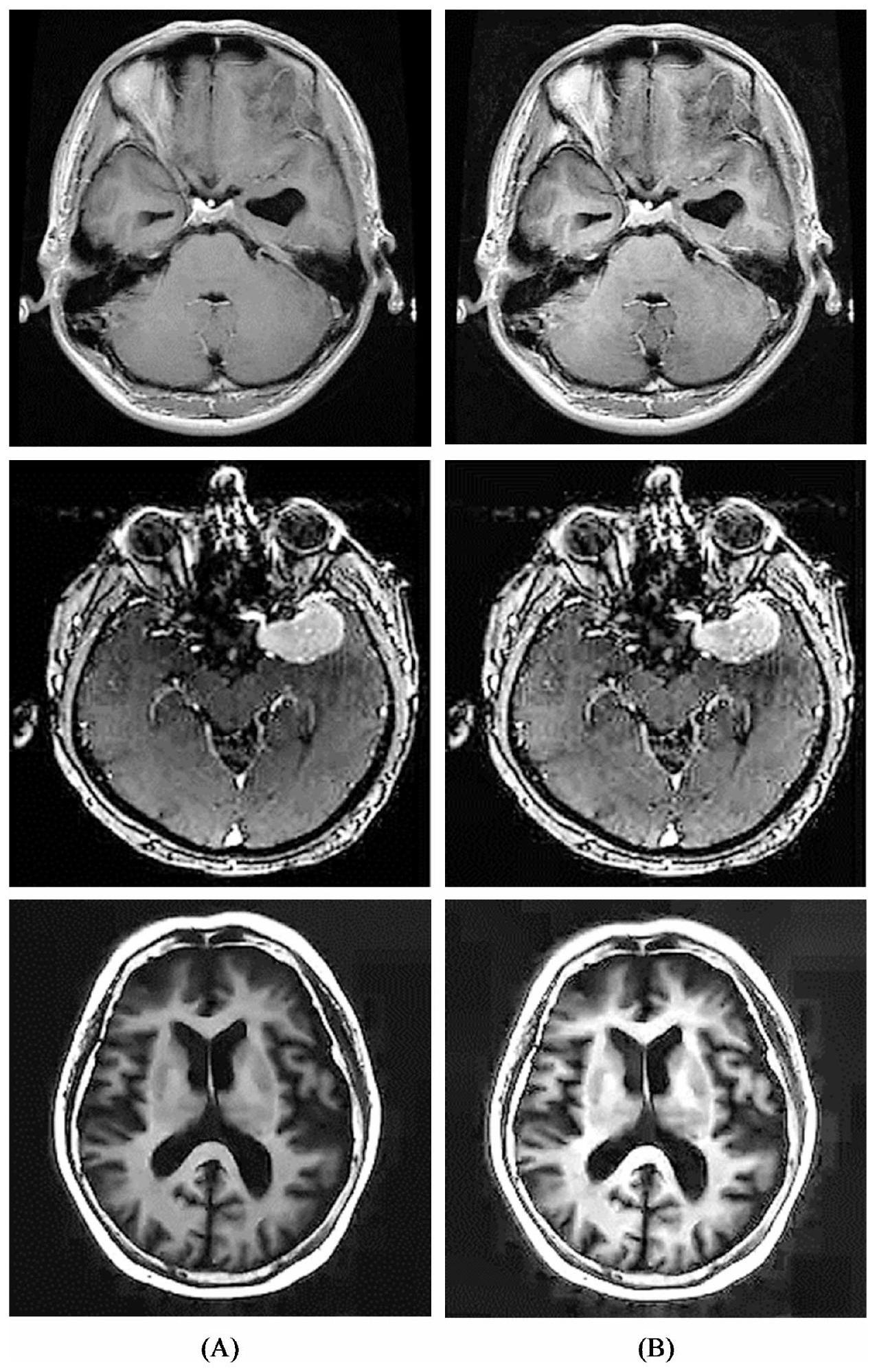
- Employing CLAHE improved the visibility and clarity of important tumor features in the MRI images, thereby enhancing the subsequent analysis and classification tasks.
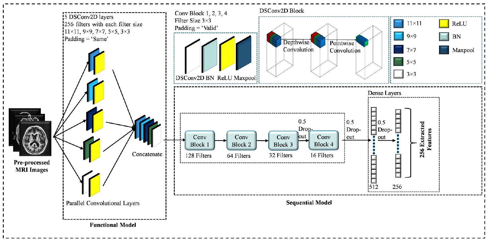
- A lightweight parallel depthwise separable CNN (PDSCNN) is proposed to extract relevant features from enhanced MRI images. This model efficiently captures tumor-specific patterns while minimizing computational complexity.
- A hybrid ridge regression ELM (RRELM) model is proposed, which enhances the traditional ELM by replacing the pseudoinverse with ridge regression for improved classification performance.
- This study compared the proposed framework with various state-of-the-art (SOTA) models based on classification performance, model parameters, and layer sizes.
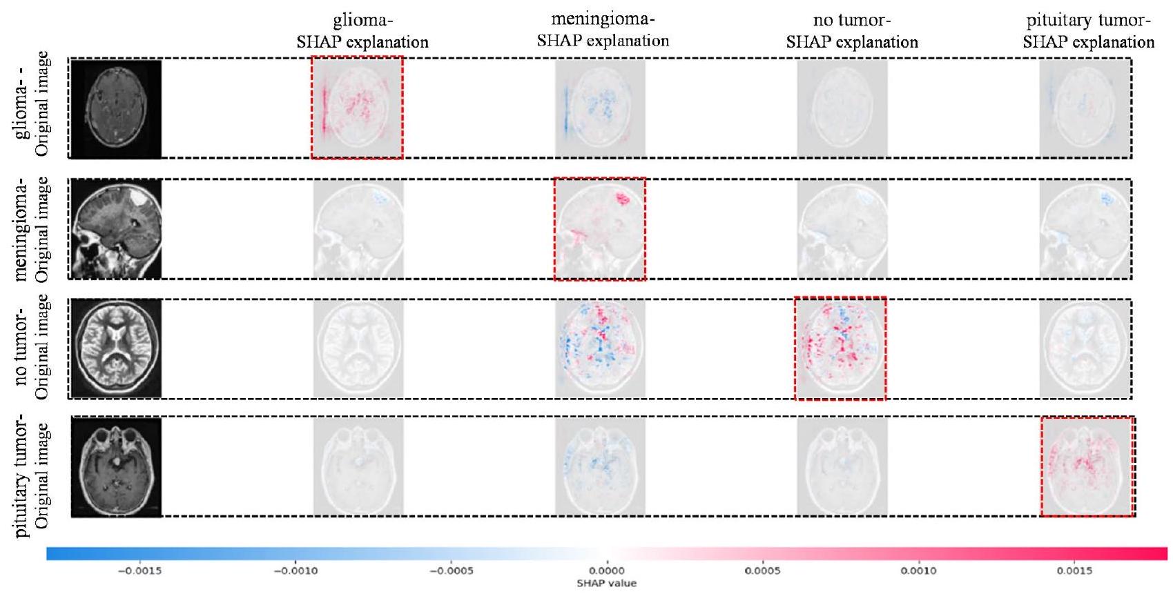
- The interpretability of the framework is showcased by employing SHAP, which allows a deeper understanding of the model’s decision making, increasing confidence in its real-world diagnostic application.
Literature review
exhibited high accuracy in categorizing the limited database by incorporating dense and drop-out layers. Data augmentation and min-max normalization were combined to enhance tumor cell contrast. The experimental results demonstrated exceptional performance, with a training accuracy of
computation time by harnessing the discriminative power of a parallel depthwise separable CNN. Notably, a pioneering approach was introduced by incorporating ridge regression into the proposed hybrid ELM model, replacing the more-pseudoinverse method. This integration enhances the classification performance of the novel hybrid ridge regression ELM (RRELM) model, surpassing the capabilities of previous approaches. In addition, conventional research boundaries were surpassed by achieving an unprecedented level of interpretability within the proposed framework. By developing a hybrid explainable CNN-ELM, the authors gained insights into the inner workings of the proposed model, allowing them to decipher the specific image regions that contribute most prominently to the classification of brain tumors. Transfer learning has emerged as a pivotal approach in image representation, particularly in fields with limited labeled data. The survey on food category recognition Zhang et al.
Methodology
Proposed framework
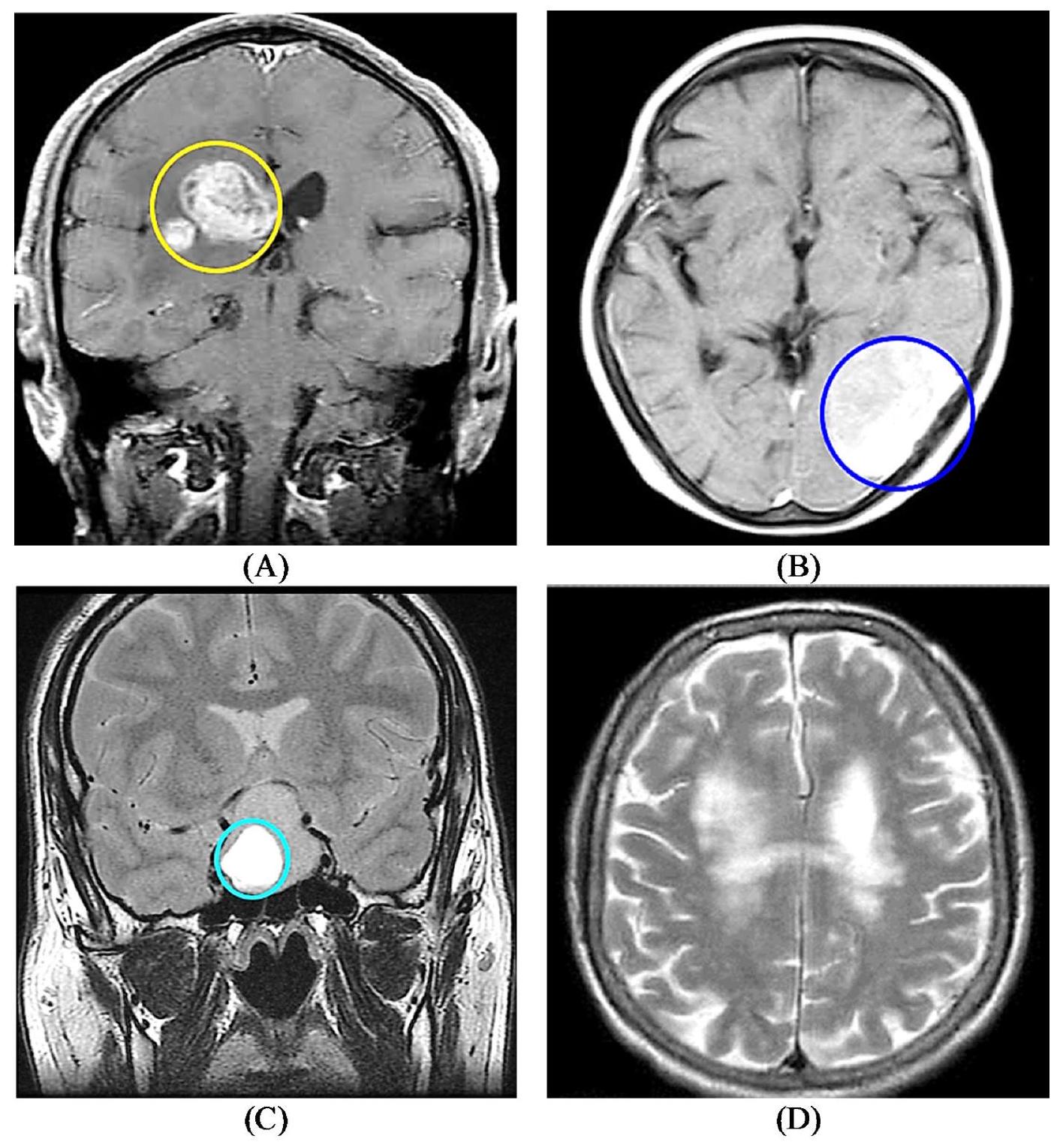
Brain tumor dataset
Data preprocessing
Parallel depthwise separable convolutional neural network
Algorithm 1
Input:
k : number of parallel kernels
s : size of each parallel kernel (an array of length k )
c: number of channels
filter_heights: height of the filter for each parallel kernel (an array of length k )
filter_widths: width of the filter for each parallel kernel (an array of length k )
Output:
num filters_concat: number of filters in the concatenated layer
total parameters: total number of parameters in the parallel layers
Procedure:
- Set num_filters_concat
- Set total_parameters
- For
to k :
a. Set filter_areafilter_heights[i] * filter_widths[i]
b. Set depthwise_params* filter_heights[i] * filter_widths[i]
c. Set pointwise params
d. If it is separable convolution:
e. If it is normal convolution:
f. Add p to total parameters
4. Return num _filters_concat, total_parameters
Interaction between PDSCNN and RRELM
t-SNE Visualization in 3D
Ridge regression extreme learning machine
Initialization: The input weight matrix (input_weights) of size (input_size × hidden_size) and biases were randomly initialized using a normal distribution.
Activation function: The rectified linear unit (ReLU) function was used as the activation function for the hidden layer. It can be defined as
Hidden layer computation: The hidden_nodes() function computes the hidden layer output (H_train) using the following equations.
H_train
output_weights = inv (H_train. T @ H_train + alpha * I) @ H_train. T @ y_train, where alpha is the regularization parameter, I represents the identity matrix of size hidden_size, and y_train denotes the target labels.
Prediction : The predict() function was introduced to make predictions using the trained model. It computes the output of the hidden layer for the given input features ( X ) using the following equations.
predictions
By incorporating Ridge Regression within the ELM (RRELM) framework, this methodology aimed to strike a balance between effective feature learning and regularization, enhancing the model’s ability to generalize and produce accurate predictions.
Assessment matrices and implementation
Results and discussion
An ELM with pseudoinverse
ELM with ridge regression
| Fold number | Diseases name | Precision | Recall | F1-score | Accuracy (%) |
| Fold 1 | Glioma (0) | 0.99 | 0.99 | 0.99 | – |
| Meningioma (1) | 0.99 | 0.98 | 0.99 | – | |
| No Tumor (2) | 1.00 | 1.00 | 1.00 | – | |
| Pituitary (3) | 0.99 | 0.99 | 0.99 | – | |
| Average | 0.9925* | 0.99 | 0.9925 | 99.21 | |
| Fold 2 | Glioma (0) | 0.99 | 0.99 | 0.99 | – |
| Meningioma (1) | 0.98 | 0.99 | 0.98 | – | |
| No Tumor (2) | 1.00 | 1.00 | 1.00 | – | |
| Pituitary (3) | 0.99 | 1.00 | 0.99 | – | |
| Average | 0.99 | 0.9950 | 0.99 | 99.21 | |
| Fold 3 | Glioma (0) | 0.99 | 0.99 | 0.99 | – |
| Meningioma (1) | 0.98 | 0.98 | 0.98 | – | |
| No Tumor (2) | 1.00 | 1.00 | 1.00 | – | |
| Pituitary (3) | 1.00 | 0.99 | 1.00 | – | |
| Average | 0.9925 | 0.99 | 0.9925 | 99.14 | |
| Fold 4 | Glioma (0) | 0.98 | 0.98 | 0.98 | – |
| Meningioma (1) | 0.99 | 0.98 | 0.98 | – | |
| No Tumor (2) | 1.00 | 1.00 | 1.00 | – | |
| Pituitary (3) | 0.99 | 1.00 | 0.99 | – | |
| Average | 0.99 | 0.99 | 0.9875 | 99.00 | |
| Fold 5 | Glioma (0) | 1.00 | 0.98 | 0.99 | – |
| Meningioma (1) | 0.97 | 0.99 | 0.98 | – | |
| No Tumor (2) | 1.00 | 1.00 | 1.00 | – | |
| Pituitary (3) | 0.99 | 0.99 | 0.99 | – | |
| Average | 0.99 | 0.99 | 0.99 | 99.07 |
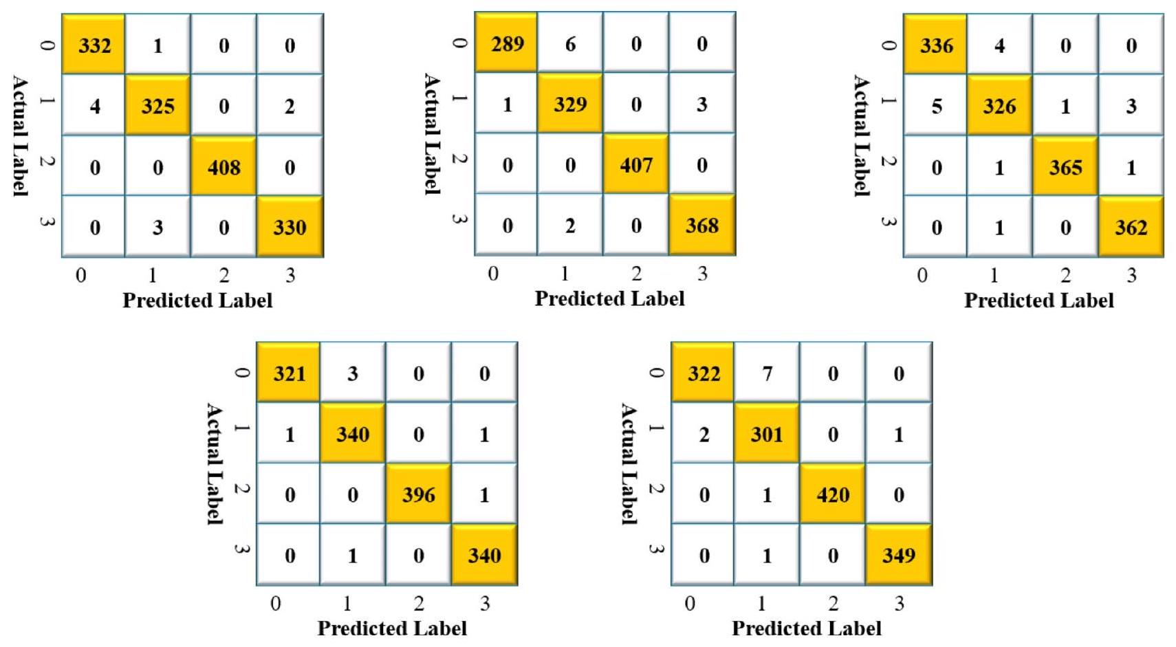
Comparison between PELM and RRELM
| Fold number | Diseases Name | Precision | Recall | F1-score | Accuracy (%) |
| Fold 1 | Glioma (0) | 0.99 | 1.00 | 0.99 | – |
| Meningioma (1) | 0.99 | 0.98 | 0.98 | – | |
| No Tumor (2) | 1.00 | 1.00 | 1.00 | – | |
| Pituitary (3) | 0.99 | 0.99 | 0.99 | – | |
| Average | 0.9925 | 0.9925 | 0.99 | 99.28 | |
| Fold 2 | Glioma (0) | 1.00 | 0.98 | 0.99 | – |
| Meningioma (1) | 0.98 | 0.99 | 0.98 | – | |
| No Tumor (2) | 1.00 | 1.00 | 1.00 | – | |
| Pituitary (3) | 0.99 | 0.99 | 0.99 | – | |
| Average | 0.9925 | 0.99 | 0.99 | 99.14 | |
| Fold 3 | Glioma (0) | 0.99 | 0.99 | 0.99 | – |
| Meningioma (1) | 0.99 | 0.98 | 0.98 | – | |
| No Tumor (2) | 1.00 | 0.99 | 1.00 | – | |
| Pituitary (3) | 0.99 | 1.00 | 0.99 | – | |
| Average | 0.9925 | 0.9925 | 0.99 | 99.04 | |
| Fold 4 | Glioma (0) | 1.00 | 0.99 | 0.99 | – |
| Meningioma (1) | 0.99 | 0.99 | 0.98 | – | |
| No Tumor (2) | 1.00 | 1.00 | 1.00 | – | |
| Pituitary (3) | 0.99 | 1.00 | 1.00 | – | |
| Average | 1.00* | 1.00 | 1.00 | 99.50 | |
| Fold 5 | Glioma (0) | 0.99 | 0.98 | 0.99 | – |
| Meningioma (1) | 0.97 | 0.99 | 0.98 | – | |
| No Tumor (2) | 1.00 | 1.00 | 1.00 | – | |
| Pituitary (3) | 1.00 | 1.00 | 1.00 | – | |
| Average | 0.99 | 0.9925 | 0.9925 | 99.14 |
| Model name | Precision average
|
Recall
|
F1-score
|
Accuracy
|
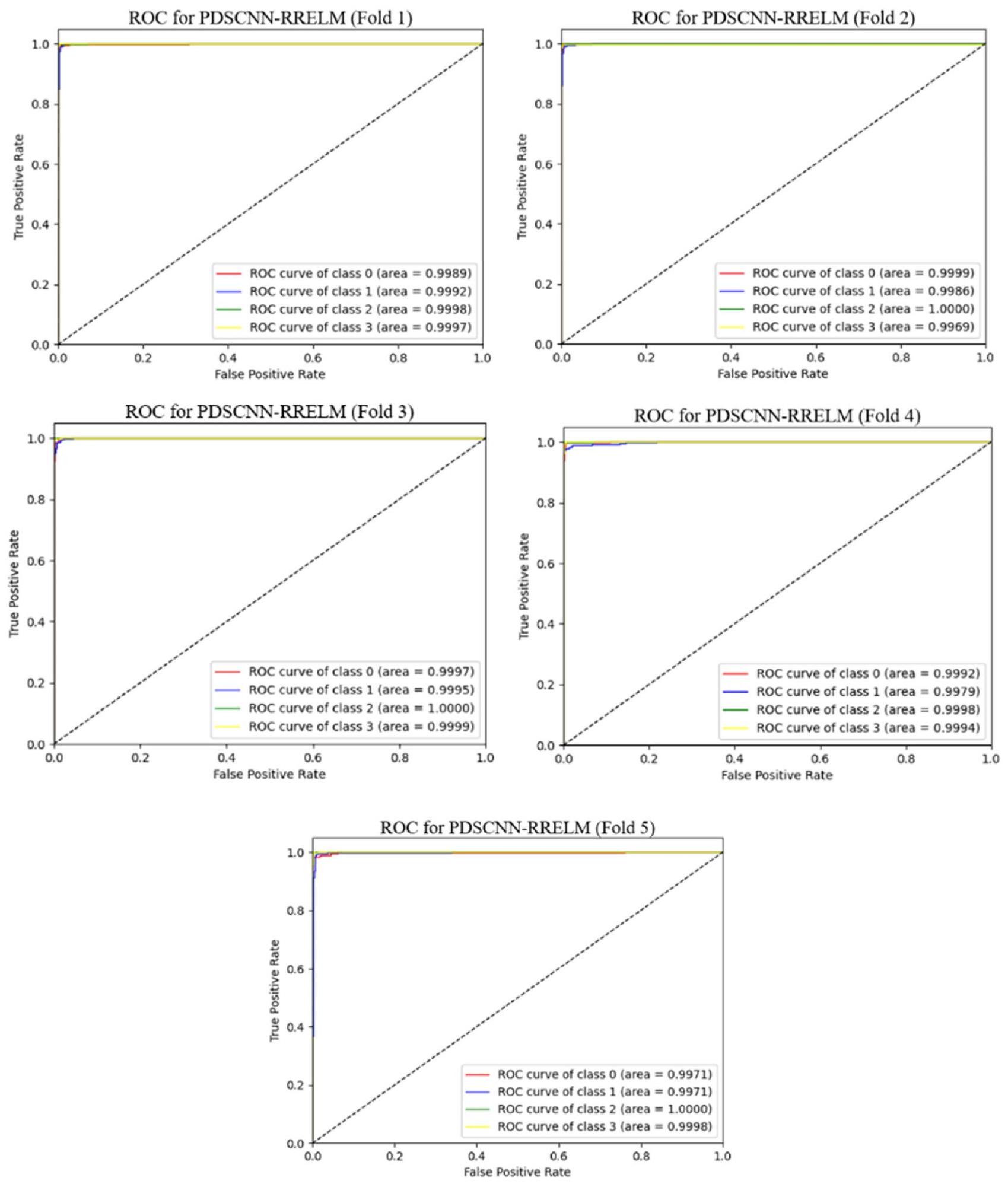
AUC
|
| PDSCNN-PELM |
|
|
|
|
|
| PDSCNN-RRELM |
|
|
|
|
|
Performances comparison of PDSCNN-RRELM with SOTA models
Interpretability of PDSCNN-RRELM using SHAP
| Reference | Dataset size | Target class | Precision (%) | Recall (%) | F1-score (%) | Accuracy (%) | AUC (%) | Para-meters (million) | Layers | Model |
| Gumaei et al.
|
Train: 2145 Test: 919 | 3 | – | – | – | 94.233 | – | – | – | RELM |
| Mzoughi et al.
|
Train: 284 Test: 67 | 2 | – | – | – | 96.49 | – | – | – | 3D CNN |
| Khan et al.
|
Train: 2840 Test: 424 | 3 | 99.13 | – | – | 99.13 | – | – | – | HDL2BT |
| Ahmed et al.
|
Train: 2968 Test: 394 Val: 32 | 4 | – | 96.34 | 98.22 | 97.98 | – | 14 | Custom CNN | |
| Nayak et al.
|
Train: 2608 Test: 652 | 3 | 98.75 | 98.75 | 98.75 | 98.78 | – | 5.3 | 230 | Variant of EfficientNet |
| Alanazi et al.
|
Train: 1980 Test: 495 | 3 | – | – | – | 96.89 | – | – | 22 | Transfer deep learning |
| Badza et al.
|
Train: 2758 Test: 306 | 3 | 97.15 | 97.82 | 97.47 | 97.28 | – | – | 22 | Custom CNN |
| Deepak et al.
|
Train: 2450 Test: 614 | 3 | 97.30 | 97.60 | 97.00 | 97.10 | 99.70 | 6.6 | 22 | Deep transfer learning |
| Shaik et al.
|
Train: 2450 Test: 614 | 3 | 96.14 | 95.99 | 96.03 | 96.51 | 99.00 | 2.4 | 53 | MANet |
| Ferdous et al.
|
Train: 5156 Test: 1031 | 3 | – | – | – | 98.11 | – | 8 | 14 | LCDEiT |
| Reddy et al.
|
Train: 5712 Test: 1311 | 4 | 98.6 | 98.6 | 98.6 | 98.7 | – | – | 32 | FTVT-b32 |
| Wang et al.
|
Train: 5800 Test: 1400 | 4 | 98.87 | 98.46 | 98.66 | 98.86 | – | – | 12 | RanMer-Former |
| Proposed work | Train:5619 Test:1404 | 4 | 99.35* | 99.30 | 99.25 | 99.22 | 99.99 | 0.53 | 10 | PDSCNN-RRELM |
Published online: 10 January 2025
References
- Louis, D. N. et al. The 2016 World Health Organization classification of tumors of the central nervous system: A summary. Acta Neuropathol. 131, 803-820 (2016).
- Chahal, P. K., Pandey, S. & Goel, S. A survey on brain tumor detection techniques for MR images. Multimed. Tools Appl. 79, 21771-21814 (2020).
- Guan, Y. et al. A framework for efficient brain tumor classification using MRI images (2021).
- Komninos, J. et al. Tumors metastatic to the pituitary gland: Case report and literature review. J. Clin. Endocrinol. Metab. 89, 574-580 (2004).
- Ahamed, M. F. et al. A review on brain tumor segmentation based on deep learning methods with federated learning techniques. Comput. Med. Imaging Graph. 110, 102313 (2023).
- Faysal Ahamed, M., Robiul Islam, M., Hossain, T., Syfullah, K. & Sarkar, O. Classification and segmentation on multi-regional brain tumors using volumetric images of MRI with customized 3D U-Net framework. In Proceedings of International Conference on Information and Communication Technology for Development: ICICTD 2022 223-234 (Springer, 2023).
- Titu, M. M. T., Mary, M. M., Ahamed, M. F., Oishee, T. M. & Hasan, M. M. Utilizing customized 3D U-Net framework for the classification and segmentation of multi-regional brain tumors in volumetric MRI images. In 2024 3rd International Conference on Advancement in Electrical and Electronic Engineering (ICAEEE) 1-6 (IEEE, 2024).
- Ahamed, M. F. et al. Automated detection of colorectal polyp utilizing deep learning methods with explainable AI. IEEE Access (2024).
- Varuna Shree, N. & Kumar, T. N. R. Identification and classification of brain tumor MRI images with feature extraction using DWT and probabilistic neural network. Brain Inf. 5, 23-30 (2018).
- Nahiduzzaman, M., Islam, M. R. & Hassan, R. ChestX-Ray6: Prediction of multiple diseases including COVID-19 from chest X-ray images using convolutional neural network. Expert Syst. Appl. 211, 118576 (2023).
- Islam, M. R. & Nahiduzzaman, M. Complex features extraction with deep learning model for the detection of COVID19 from CT scan images using ensemble based machine learning approach. Expert Syst. Appl. 195, 116554 (2022).
- Nahiduzzaman, M. et al. Diabetic retinopathy identification using parallel convolutional neural network based feature extractor and ELM classifier. Expert Syst. Appl. 217, 119557 (2023).
- Nahiduzzaman, M. et al. Hybrid CNN-SVD based prominent feature extraction and selection for grading diabetic retinopathy using extreme learning machine algorithm. IEEE Access 9, 152261-152274 (2021).
- Nahiduzzaman, M. et al. A novel method for multivariant pneumonia classification based on hybrid CNN-PCA based feature extraction using extreme learning machine with CXR images. IEEE Access 9, 147512-147526 (2021).
- Hossain, M. M., Islam, M. R., Ahamed, M. F., Ahsan, M. & Haider J. A collaborative federated learning framework for lung and colon cancer classifications. Technologies 12, 151 (2024).
- Hossain, M. M., Ahamed, M. F., Islam, M. R. & Imam, M. D. R. Privacy preserving federated learning for lung cancer classification. In 2023 26th International Conference on Computer and Information Technology (ICCIT) 1-6 (IEEE, 2023).
- Ahamed, M. F., Nahiduzzaman, M., Ayari, M. A., Khandakar, A. & Islam, S. M. R. Malaria parasite classification from RBC smears using lightweight parallel depthwise separable CNN and ridge regression ELM by integrating SHAP techniques (2023).
- Sarkar, O. et al. Multi-scale CNN: An explainable AI-integrated unique deep learning framework for lung-affected disease classification. Technologies 11, 134 (2023).
- Ullah, F., Nadeem, M. & Abrar, M. Revolutionizing brain tumor segmentation in MRI with dynamic fusion of handcrafted features and global pathway-based deep learning. KSII Trans. Internet Inform. Syst. 18 (2024).
- Anwar, R. W., Abrar, M. & Ullah, F. Transfer learning in brain tumor classification: Challenges, opportunities, and future prospects. In 2023 14th International Conference on Information and Communication Technology Convergence (ICTC) 24-29 (IEEE, 2023).
- Akbar, M. et al. An effective deep learning approach for the classification of Bacteriosis in peach leave. Front. Plant Sci. 13. https:/ /doi.org/10.3389/fpls.2022.1064854 (2022).
- Nazar, U. et al. Review of automated computerized methods for brain tumor segmentation and classification. Curr. Med. Imaging 16, 823-834 (2020).
- Ahamed, M. F., Sarkar, O. & Matin, A. Instance segmentation of visible cloud images based on mask R-CNN applying transfer learning approach. In 2020 2nd International Conference on Advanced Information and Communication Technology (ICAICT) 257-262 (IEEE, 2020). https://doi.org/10.1109/ICAICT51780.2020.9333531.
- Musallam, A. S., Sherif, A. S. & Hussein, M. K. A new convolutional neural network architecture for automatic detection of brain tumors in magnetic resonance imaging images. IEEE Access 10, 2775-2782 (2022).
- Simonyan, K. & Zisserman, A. Very deep convolutional networks for large-scale image recognition. arXiv preprint arXiv:1409.1556 (2014).
- Nayak, D. R., Padhy, N., Mallick, P. K., Zymbler, M. & Kumar, S. Brain tumor classification using dense efficient-net. Axioms 11, 34 (2022).
- Alanazi, M. F. et al. Brain tumor/mass classification framework using magnetic-resonance-imaging-based isolated and developed transfer deep-learning model. Sensors 22, 372 (2022).
- Khan, A. H. et al. Intelligent model for brain tumor identification using deep learning. Appl. Computat. Intell. Soft Comput. 2022, 8104054 (2022).
- Irmak, E. Multi-classification of brain tumor MRI images using deep convolutional neural network with fully optimized framework. Iran. J. Sci. Technol. Trans. Electr. Eng. 45, 1015-1036 (2021).
- Badža, M. M. & Barjaktarović, M. Č. Classification of brain tumors from MRI images using a convolutional neural network. Appl. Sci. 10, 1999 (2020).
- Mzoughi, H. et al. Deep multi-scale 3D convolutional neural network (CNN) for MRI gliomas brain tumor classification. J. Digit. Imaging 33, 903-915 (2020).
- Gumaei, A., Hassan, M. M., Hassan, M. R., Alelaiwi, A. & Fortino, G. A hybrid feature extraction method with regularized extreme learning machine for brain tumor classification. IEEE Access 7, 36266-36273 (2019).
- Deepak, S. & Ameer, P. M. Brain tumor classification using deep CNN features via transfer learning. Comput. Biol. Med. 111, 103345 (2019).
- Shaik, N. S. & Cherukuri, T. K. Multi-level attention network: Application to brain tumor classification. Signal. Image Video Process. 16, 817-824 (2022).
- Ahuja, S., Panigrahi, B. K. & Gandhi, T. K. Enhanced performance of Dark-nets for brain tumor classification and segmentation using colormap-based superpixel techniques. Mach. Learn. Appl. 7, 100212 (2022).
- Brain Tumor MRI Dataset. https://www.kaggle.com/datasets/masoudnickparvar/brain-tumor-mri-dataset/data.
- Pisano, E. D. et al. Contrast limited adaptive histogram equalization image processing to improve the detection of simulated spiculations in dense mammograms. J. Digit. Imaging 11, 193-200 (1998).
- Ahamed, M. F., Salam, A., Nahiduzzaman, M., Abdullah-Al-Wadud, M. & Islam, S. M. R. streamlining plant disease diagnosis with convolutional neural networks and edge devices. Neural Comput. Appl. 36, 18445-18477 (2024).
- Ahamed, M. F. et al. Detection of various gastrointestinal tract diseases through a deep learning method with ensemble ELM and explainable AI. Expert Syst. Appl. 256, 124908 (2024).
- Ahamed, M. F. et al. Interpretable deep learning model for tuberculosis detection using X-ray images. In Surveillance, Prevention, and Control of Infectious Diseases: An AI Perspective (eds. Chowdhury, M. E. H. & Kiranyaz, S.) 169-192 (Springer, 2024).
- Huang, G. B., Zhu, Q. Y. & Siew, C. K. Extreme learning machine: Theory and applications. Neurocomputing 70, 489-501 (2006).
- Nahiduzzaman, M. et al. Parallel CNN-ELM: A multiclass classification of chest X-ray images to identify seventeen lung diseases including COVID-19. Expert Syst. Appl. 229, 120528 (2023).
- Nahiduzzaman, M., Nayeem, M. J., Ahmed, M. T. & Zaman, M. S. U. Prediction of heart disease using multi-layer perceptron neural network and support vector machine. In 2019 4th International Conference on Electrical Information and Communication Technology (EICT) 1-6 (IEEE, 2019).
- Kibria, H. B., Nahiduzzaman, M., Goni, M. O. F., Ahsan, M. & Haider, J. An ensemble approach for the prediction of diabetes mellitus using a soft voting classifier with an explainable AI. Sensors 22, 7268 (2022).
- Powers, D. M. W. Evaluation: From precision, recall and F-measure to ROC, informedness, markedness and correlation. arXiv preprint arXiv:2010.16061(2020).
- Swets, J. A. Measuring the accuracy of diagnostic systems. Science (1979) 240, 1285-1293 (1988).
- Ferdous, G. J., Sathi, K. A., Hossain, M. A., Hoque, M. M. & Dewan, M. A. A. LCDEiT: A linear complexity data-efficient image transformer for MRI brain tumor classification. IEEE Access 11, 20337-20350 (2023).
- Reddy, C. K. K. et al. A fine-tuned vision transformer based enhanced multi-class brain tumor classification using MRI scan imagery. Front. Oncol. 141-23 (2024).
- Wang, J., Lu, S. Y., Wang, S. H. & Zhang, Y. D. RanMerFormer: Randomized vision transformer with token merging for brain tumor classification. Neurocomputing 573, 127216 (2024).
- Lundberg, S. A unified approach to interpreting model predictions. arXiv Preprint arXiv:1705.07874 (2017).
- Bhandari, M., Shahi, T. B., Siku, B. & Neupane, A. Explanatory classification of CXR images into COVID-19, Pneumonia and Tuberculosis using deep learning and XAI. Comput. Biol. Med. 150, 106156 (2022).
- Ullah, F. et al. Evolutionary model for brain cancer-grading and classification. IEEE Access 11, 126182-126194 (2023).
- Ullah, F. et al. Enhancing brain tumor segmentation accuracy through scalable federated learning with advanced data privacy and security measures. Mathematics 11, 4189 (2023).
- Ullah, F. et al. Brain tumor segmentation from MRI images using handcrafted convolutional neural network. Diagnostics 13, 2650 (2023).
- Zhang, Y. et al. Deep learning in food category recognition. Inf. Fusion 98, 101859 (2023).
- Lu, S. Y., Nayak, D. R., Wang, S. H. & Zhang Y.-D. A cerebral microbleed diagnosis method via FeatureNet and ensembled randomized neural networks. Appl. Soft Comput. 109, 107567 (2021).
- Lu, S. Y., Zhu, Z., Tang, Y., Zhang, X. & Liu, X. CTBViT: A novel ViT for tuberculosis classification with efficient block and randomized classifier. Biomed. Signal. Process. Control 100, 106981 (2025).
Author contributions
Declarations
Competing interests
Additional information
Reprints and permissions information is available at www.nature.com/reprints.
Publisher’s note Springer Nature remains neutral with regard to jurisdictional claims in published maps and institutional affiliations.
© The Author(s) 2025, corrected publication 2025
Department of Electrical and Computer Engineering, Rajshahi University of Engineering and Technology, Rajshahi 6204, Bangladesh. Department of Space Technology Engineering, Electrical Engineering Technical College, Middle Technical University, Baghdad, Iraq. Department of Computer Science, Cihan University Sulaimaniya, Sulaimaniya 46001, Kurdistan Region, Iraq. Department of Electrical Engineering, Qatar University, Doha 2713, Qatar. Department of Civil and Environmental Engineering, Qatar University, Doha 2713, Qatar. Department of Computer Science, University of York, Deramore Lane, York YO10 5GH, UK. Department of Engineering, Manchester Metropolitan University, Chester Street, Manchester M1 5GD, UK. Artificial Intelligence and Digital Health, School of Health and Rehabilitation Sciences, Faculty of Health and Behavioral Sciences, The University of Queensland, St Lucia, QLD 4072, Australia. Institute of Optoelectronics, Military University of Technology, Gen. S. Kaliskiego 2, Warsaw 00-908, Poland. email: marcin.kowalski@wat.edu.pl