نموذج هجين لشبكة عصبية عميقة لتصنيف صور أورام الدماغ متعددة الفئات A hybrid deep CNN model for brain tumor image multi-classification

المجلة: BMC Medical Imaging، المجلد: 24، العدد: 1
DOI: https://doi.org/10.1186/s12880-024-01195-7
PMID: https://pubmed.ncbi.nlm.nih.gov/38243215
تاريخ النشر: 2024-01-19

نموذج هجين لشبكة عصبية عميقة لتصنيف صور أورام الدماغ متعددة الفئات

سارافانان سريفياسان ديفيا فرانسيس سانديب كومار ماثيفانان هاريهاران راجادوراي باسو ديف شيفاهاري ومحمد عاصف شاه

الملخص

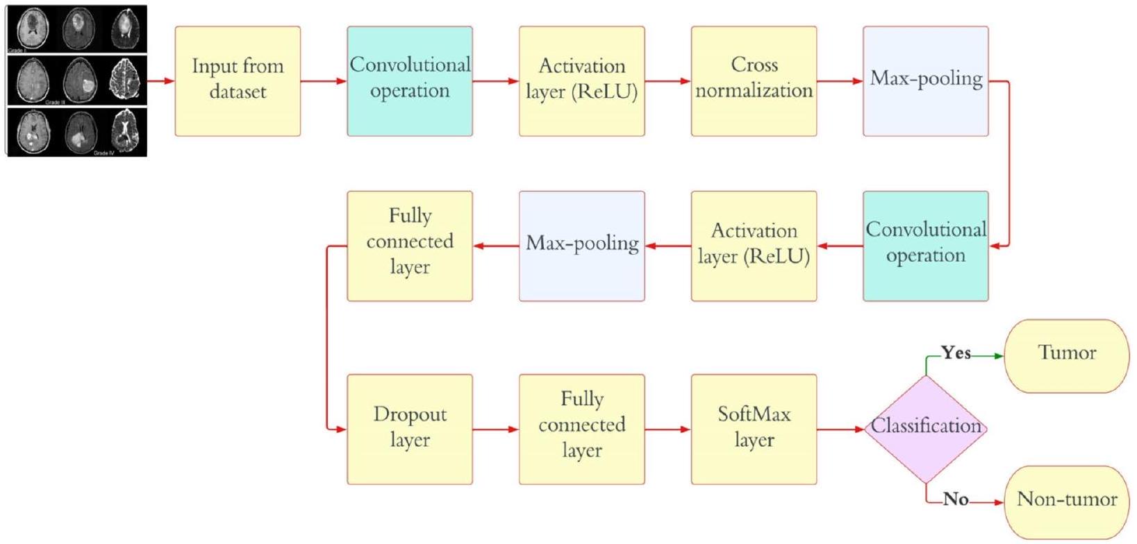
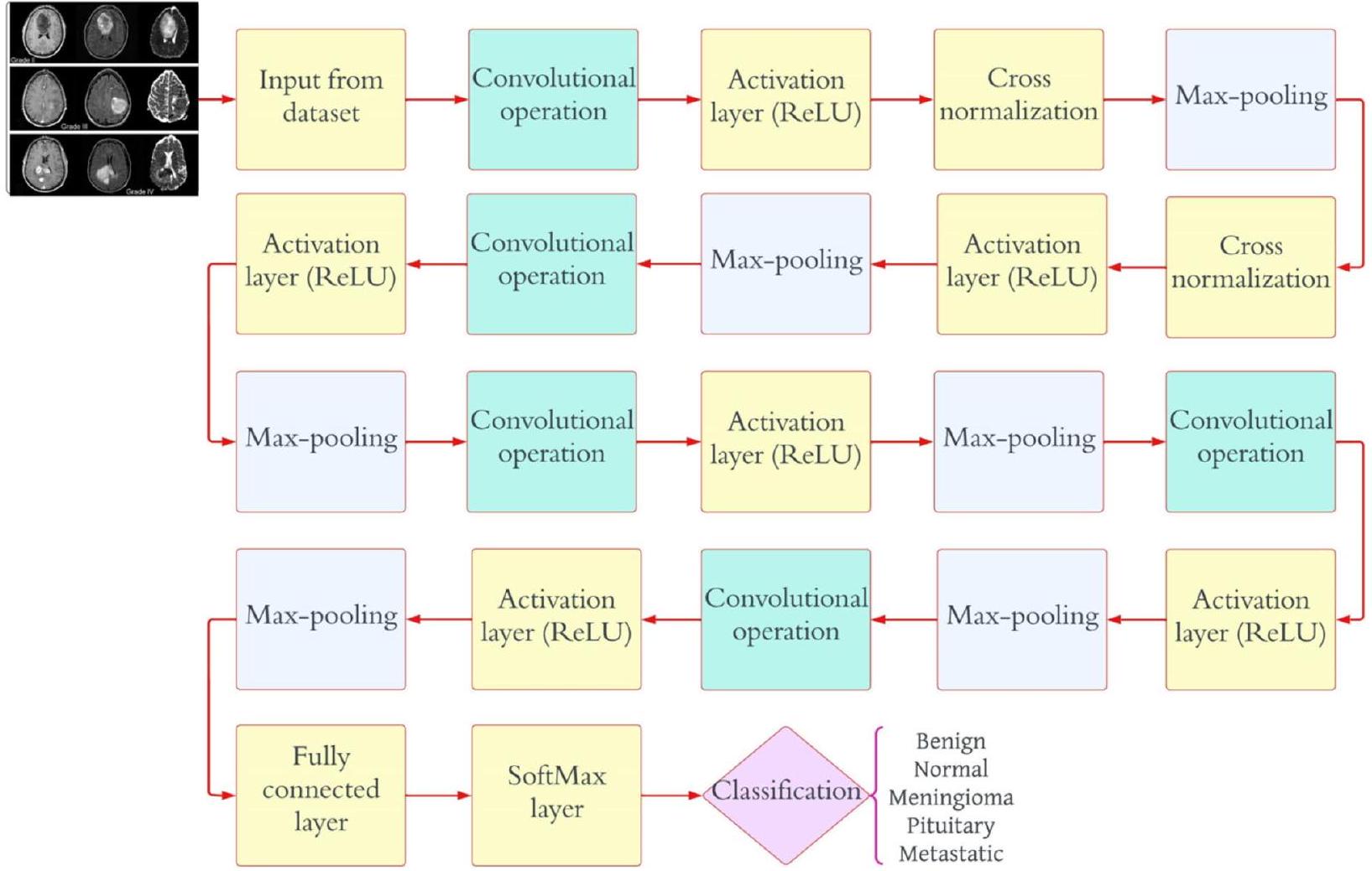
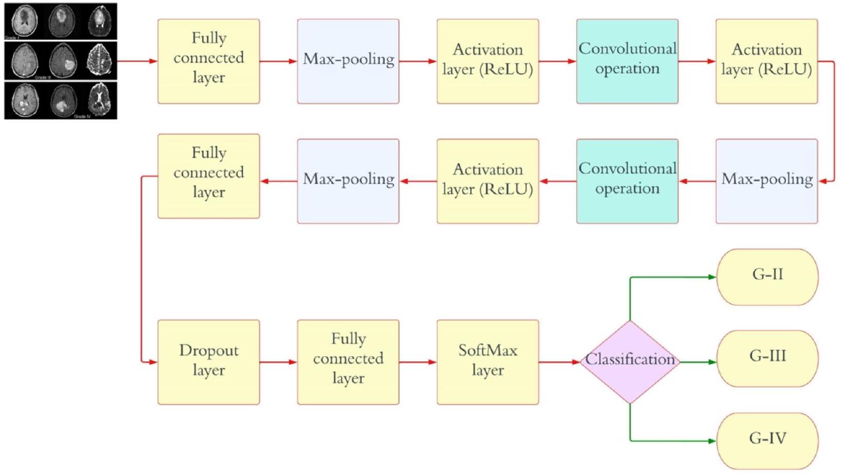
النهج الحالي لتشخيص وتصنيف أورام الدماغ يعتمد على التقييم النسيجي لعينات الخزعة، وهو نهج يتسم بالتدخل، ويستغرق وقتًا طويلاً، ويكون عرضة للأخطاء اليدوية. هذه القيود تبرز الحاجة الملحة إلى نظام تصنيف متعدد الفئات يعتمد على التعلم العميق بشكل كامل لأورام الدماغ الخبيثة. يهدف هذا المقال إلى الاستفادة من شبكة عصبية تلافيفية عميقة (CNN) لتعزيز الكشف المبكر ويقدم ثلاثة نماذج CNN متميزة مصممة لمهام تصنيف مختلفة. يحقق النموذج الأول من CNN دقة كشف مثيرة للإعجاب تبلغ 99.53% لأورام الدماغ. النموذج الثاني من CNN، بدقة تبلغ 93.81%، يصنف أورام الدماغ بكفاءة إلى خمسة أنواع متميزة: طبيعي، غليوما، منينجيوما، نخامية، وانتقالية. علاوة على ذلك، يظهر النموذج الثالث من CNN دقة تبلغ في تصنيف أورام الدماغ بدقة إلى درجاتها المختلفة. لضمان الأداء الأمثل، يتم استخدام نهج تحسين البحث الشبكي لضبط جميع المعلمات الفائقة ذات الصلة بنماذج الشبكات العصبية التلافيفية تلقائيًا. تؤدي الاستفادة من مجموعات البيانات السريرية الكبيرة والمتاحة للجمهور إلى نتائج تصنيف قوية وموثوقة. يجري هذا المقال مقارنة شاملة للنماذج المقترحة مقابل النماذج الكلاسيكية، مثل AlexNet وDenseNet121 وResNet-101 وVGG-19 وGoogleNet، مما يؤكد تفوق النهج القائم على الشبكات العصبية التلافيفية العميقة في تقدم مجال تصنيف أورام الدماغ والكشف المبكر.

الكلمات الرئيسية: تصنيف ورم الدماغ، التعلم العميق الهجين، الشبكة العصبية التلافيفية الهجينة، بحث الشبكة، المعلمات الفائقة

مقدمة

تشكل أورام الدماغ واحدة من الأسباب الرئيسية للوفاة في العالم الحديث. يمكن أن تظهر هذه الأورام في مناطق مختلفة من الدماغ، وغالبًا ما تظل بدون أعراض حتى مراحل متأخرة من الحياة. تشمل أعراض أمراض الدماغ مجموعة واسعة من المشكلات، بما في ذلك تغييرات في الشخصية، صعوبات في الذاكرة، ضعف في التواصل، تحديات في السمع أو الكلام، صداع نصفي مزمن، وحتى فقدان الرؤية. تشمل الأمثلة البارزة على أورام الدماغ الأورام السحائية، الأورام الدبقية، الأورام الغدية النخامية، والأورام العصبية السمعية. وفقًا للملاحظات الطبية، تمثل الأورام السحائية، الأورام الدبقية، وأورام الغدة النخامية حوالي ، و من جميع أورام الدماغ، على التوالي. يمكن أن يكون لورم الدماغ آثار نفسية طويلة الأمد على المريض. تنشأ هذه الأورام من اضطرابات أولية في الدماغ.
أو نسيج العمود الفقري المركزي الذي يعطل الوظيفة الطبيعية للدماغ. يتم تصنيف أورام الدماغ إلى فئتين رئيسيتين: حميدة وخبيثة. تنمو الأورام الحميدة ببطء وهي غير سرطانية؛ وهي نادرة نسبيًا ولا تنتشر. بالمقابل، تحتوي أورام الدماغ الخبيثة على خلايا سرطانية، وعادة ما تنشأ في منطقة واحدة من الدماغ قبل أن تنتشر بسرعة إلى مناطق أخرى من الدماغ والحبل الشوكي [2]. تشكل الأورام الخبيثة خطرًا صحيًا كبيرًا. تصنف منظمة الصحة العالمية (WHO) أورام الدماغ إلى أربع درجات بناءً على سلوكها داخل الدماغ: تعتبر الدرجات 1 و 2 أورامًا منخفضة الدرجة أو حميدة، بينما تصنف الدرجات 3 و 4 كأورام عالية الدرجة أو خبيثة. تتوفر عدة طرق تشخيصية، مثل التصوير المقطعي المحوسب (CT) وتخطيط كهربية الدماغ (EEG)، للكشف عن أورام الدماغ، لكن التصوير بالرنين المغناطيسي (MRI) هو الأكثر موثوقية واستخدامًا على نطاق واسع. ينتج التصوير بالرنين المغناطيسي صورًا داخلية مفصلة لأعضاء الجسم من خلال استخدام مجالات مغناطيسية قوية وموجات راديو [3]. بشكل أساسي، يمكن أن تميز فحوصات CT أو MRI المنطقة المتأثرة في الدماغ بسبب الورم عن الأنسجة السليمة. يمكن إجراء خزعات، وهي اختبارات سريرية تستخرج خلايا الدماغ، كتمهيد لجراحة الدماغ. الدقة أمر بالغ الأهمية في قياس خلايا الورم أو الوصول إلى تشخيصات دقيقة. يمثل ظهور التعلم الآلي (ML) فرصة لمساعدة أطباء الأشعة في تقديم معلومات دقيقة عن حالة المرض [4]. لقد تركت وفرة التقنيات الجديدة، وخاصة الذكاء الاصطناعي والتعلم الآلي، أثرًا لا يمحى في المجال الطبي، مما زود مختلف الأقسام الطبية، بما في ذلك التصوير الطبي، بأدوات لا غنى عنها لتعزيز عملياتها. بينما تتم معالجة صور الرنين المغناطيسي لمساعدة أطباء الأشعة في اتخاذ القرارات، يتم استخدام مجموعة متنوعة من استراتيجيات التعلم الآلي الآلي لأغراض التصنيف والتجزئة. بينما تحمل الطرق المراقبة لتصنيف أورام الدماغ وعدًا هائلًا، فإنها تتطلب خبرة متخصصة لتحسين تقنيات استخراج واختيار الميزات [5]. في التنقل وتحليل مجموعات البيانات الضخمة، يستفيد المتخصصون الطبيون الخبراء من دعم المساعدة الآلية. علاوة على ذلك، فإن الفشل في تحديد الأورام المهددة للحياة بدقة قد يؤدي إلى تأخيرات في العلاج للمرضى. لقد كانت تقنيات التعلم العميق (DL) في الكشف عن أورام الدماغ واستخراج رؤى ذات مغزى من أنماط البيانات لها تاريخ طويل. إن قدرة التعلم العميق على تصنيف ونمذجة سرطانات الدماغ معترف بها على نطاق واسع [6]. يعتمد علاج أورام الدماغ بشكل فعال على التشخيص المبكر والدقيق للمرض. تتأثر القرارات المتعلقة بطرق العلاج بعوامل مثل النوع المرضي للورم، والدرجة، والمرحلة عند التشخيص. لقد استغل أطباء الأورام العصبية أدوات التشخيص المدعومة بالحاسوب (CAD) لأغراض متنوعة، بما في ذلك الكشف عن الورم، والتصنيف، والتدرج ضمن مجال الأعصاب [7].
الورم الدبقي هو نوع من الأورام التي تنشأ في نسيج الدماغ، متميزة عن خلايا الأعصاب أو الأوعية الدموية. بالمقابل، تتطور الأورام السحائية من الأغشية الواقية التي تحيط بالدماغ والجهاز العصبي المركزي، بينما تنمو الأورام النخامية داخل حدود الجمجمة. من بين هذه الأنواع الثلاثة من الأورام، تعتبر الأورام السحائية نادرة نسبيًا وعادة ما تكون حميدة. على النقيض من ذلك، تشكل الأورام الدبقية الشكل الأكثر شيوعًا من الأورام الدماغية الخبيثة. على الرغم من أن الأورام النخامية قد تكون حميدة، إلا أنها لا تزال يمكن أن تؤدي إلى مضاعفات طبية كبيرة. تصنف أورام الدماغ كأحد الأسباب الرئيسية للوفيات على مستوى العالم. تؤكد الأبحاث على أهمية التعرف المبكر والدقيق، جنبًا إلى جنب مع العلاج الفوري، في تحسين معدلات البقاء على قيد الحياة للمرضى الذين يعانون من الأورام السرطانية. في بعض الحالات، قد يواجه المتخصصون في الرعاية الصحية الحاجة إلى التمييز بين السكتات الدماغية والأورام. ومن ثم، فإن الكشف المبكر عن أورام الدماغ يأخذ أهمية حيوية لتقديم رعاية فعالة وإمكانية إطالة عمر الفرد المتأثر. الشبكات العصبية التلافيفية (CNNs)، المتميزة بهيكلها متعدد الطبقات ودقتها التشخيصية العالية عند تزويدها بعدد كافٍ من صور الإدخال، تعتبر حاليًا نهجًا فعالًا للغاية في معالجة الصور. تُستخدم الشبكات العصبية، بما في ذلك المحولات الذاتية، وهي تقنية تعلم غير خاضعة للإشراف، في تعلم التمثيل. تظهر التصوير بالرنين المغناطيسي (MRI) كأداة استثنائية للحصول على تصورات واضحة ومفصلة داخل جسم الإنسان. على عكس الأشعة السينية أو الأشعة المقطعية التي تتضمن إشعاعًا مؤينًا، يوفر التصوير بالرنين المغناطيسي تباينًا محسّنًا بشكل كبير بين الأنسجة الرخوة المختلفة. علاوة على ذلك، توفر تقنية التصوير بالرنين المغناطيسي صورًا مفصلة من زوايا متعددة، مما يوفر للأطباء الإشعاعيين بيانات وفيرة حول تشريح الأنسجة الرخوة البشرية. الهدف من هذه الورقة هو تقديم ثلاثة نماذج CNN تلقائية بالكامل مصممة للتصنيف المتعدد لأورام الدماغ، باستخدام مجموعات بيانات متاحة للجمهور. حسب علم المؤلفين، يمثل هذا أول جهد في تصنيف أورام الدماغ من صور التصوير بالرنين المغناطيسي باستخدام CNNs، حيث يتم ضبط جميع المعلمات الفائقة تقريبًا تلقائيًا من خلال مُحسِّن البحث الشبكي. بقية هذه الورقة منظمة على النحو التالي: قسم المقدمة: يقدم هذا القسم نظرة شاملة على أنواع الأورام المختلفة وطرق تشخيصها؛ قسم الأعمال ذات الصلة: في هذا القسم، نتناول المقالات الحديثة، وندرس طرقها ونتائجها وتطبيقاتها؛ قسم المواد والأساليب: هنا، نفصل استخدام مجموعات البيانات ونصف هياكل النماذج المقترحة؛ قسم الدراسة التجريبية: يركز هذا القسم على تحليل مقارن للدقة التي حققتها طريقتنا المقترحة وغيرها من الأساليب المتطورة؛ الاستنتاجات.
القسم: يقدم هذا القسم الملاحظات الختامية والرؤى المتعلقة بالنموذج المقترح لدينا.
كان هدف المؤلف هو وضع نهج تصنيف يتميز بدقة أكبر، وفعالية من حيث التكلفة، وقدرة على التعلم الذاتي، من خلال استخدام مجموعة واسعة من مجموعات البيانات الأصلية بدلاً من البيانات المعززة. تم استخدام بنية VGG-16 (مجموعة الهندسة البصرية) المخصصة لتصنيف 10,153 صورة MRI إلى ثلاث فئات متميزة (غليوما، منينجيوما، وغدة نخامية). أظهر الشبكة أداءً ملحوظًا، محققة دقة إجمالية قدرها ومعدلات الدقة لـ لأورام الدبقية، لأورام السحايا، و للغدد النخامية [12]. تم تقييم فعالية النموذج المقترح باستخدام ثلاثة نماذج CNN: AlexNet وVisual Geometry Group (VGG)-16 وVGG-19. حقق AlexNet دقة اكتشاف قصوى بلغت 99.55% باستخدام 349 صورة مأخوذة من قاعدة بيانات الصور المرجعية لتقييم الاستجابة (RIDER) لقاعدة بيانات التصوير بالرنين المغناطيسي العصبي. بالنسبة لتحديد موقع ورم الدماغ، تم استخدام 804 صور رنين مغناطيسي ثلاثية الأبعاد من قاعدة بيانات تقسيم أورام الدماغ (BraTS) 2013، وتم تحقيق درجة Dice تبلغ 0.87 [13]. في دراسة تصنيف أورام الدماغ، تم استخدام مجموعة من تقنيات التعلم العميق والآلي، بما في ذلك softmax، والغابة العشوائية، وآلة الدعم الناقل (SVM)، وأقرب الجيران، وطريقة التجميع. تم مقارنة هذه النتائج مع الطرق الحالية. ومن الجدير بالذكر أن نموذج Inception-v3 أظهر أعلى أداء، محققًا دقة اختبار تبلغ . هذا التقدم يحمل القدرة على تأسيس دور بارز في التطبيقات السريرية لتحليل أورام الدماغ [14]. تم اقتراح نهج فعال لتصنيف صور الرنين المغناطيسي للدماغ إلى أربع فئات: طبيعية وثلاثة أشكال من الأورام الخبيثة في الدماغ (الورم الدبقي، الساركومة، والسرطان النقيلي المنشأ من الرئة). يدمج الأسلوب تحويل الموجات المتقطعة (DWT) مع شبكة عصبية عميقة (DNN). باستخدام مصنف شبكة عصبية عميقة، وهو أحد تصاميم التعلم العميق، تم تصنيف مجموعة بيانات مكونة من 66 صورة رنين مغناطيسي للدماغ إلى الفئات المحددة. أدى دمج DWT، وهي تقنية قوية لاستخراج الميزات، وتحليل المكونات الرئيسية (PCA)، والمصنف إلى تحقيق أداء جيد عبر جميع مقاييس التقييم [15]. قدم المؤلف استراتيجية تتضمن شبكة عصبية تلافيفية (CNN) لتمييز أورام الدماغ من صور الرنين المغناطيسي ثنائية الأبعاد للدماغ. يتبع هذا الفصل الأولي تطبيق المصنفات التقليدية وتقنيات التعلم العميق. بالإضافة إلى ذلك، تم استخدام مصنف SVM، إلى جانب خوارزميات تنشيط مختلفة، مثل softmax وRMSProp وsigmoid، للتحقق من صحة النهج المقترح ومراجعته. تم تنفيذ الحل المقترح من قبل المؤلف.
باستخدام TensorFlow و Keras في لغة البرمجة بايثون، التي تم اختيارها لقدراتها القوية في تسريع المهام. كانت نسبة الدقة المحققة لنموذج CNN عند مستوى مثير للإعجاب [16]. تقدم هذه الورقة نهجًا لتصنيف أورام الدماغ باستخدام مجموعات بيانات مفتوحة الوصول وتقنيات الشبكات العصبية التلافيفية (CNN). تستخدم المنهجية مجموعات بيانات مفتوحة الوصول لتصنيف الأنسجة كأورام أو غير أورام من خلال إطار عمل مميز يجمع بين دمج الصور المعتمد على تحويل كوساين المنفصل، وتحسين دقة الصور باستخدام الشبكات العصبية التلافيفية، ومصنف. باستخدام تحسين الدقة وهندسة ResNet50، حقق الإطار دقة مثيرة للإعجاب بلغت 98.14% [17].
تم اقتراح نهج جديد لتقليل الأبعاد، باستخدام مُحسِّن الذئب الرمادي (GWO) ونظرية المجموعات الخشنة. تحدد هذه الطريقة الميزات ذات الصلة من الصور المستخرجة، مميزة بين الأورام الدبقية متعددة الأشكال عالية الدرجة (HG) ومنخفضة الدرجة (LG) مع مراعاة قيود ارتباط الميزات لإزالة السمات الزائدة. بالإضافة إلى ذلك، يقدم المقال بنية ديناميكية لنمذجة الطبقات متعددة المستويات في نهج Faster R-CNN (MLL-CNN). يتم تحقيق ذلك باستخدام عامل وزن الميزات ونموذج وصف نسبي لبناء الميزات المختارة، مما يسهل معالجة وتصنيف الملفات ذات الذيل الطويل. يؤدي هذا التقدم إلى تحسين دقة التدريب لشبكات CNN. توضح النتائج أن التنبؤ بالنجاة العامة لنمو الدماغ GBM يحقق دقة أعلى تبلغ 95% ومعدل خطأ أقل من [18]. يتضمن العمل تصنيف 253 صورة رنين مغناطيسي للدماغ عالية الدقة إلى فئات طبيعية وفئات مرضية. لتدريب نماذج الشبكات العصبية العميقة بكفاءة ودقة، تم تعديل صور الرنين المغناطيسي من حيث الحجم، والقص، والمعالجة المسبقة، والتحسين. تم مقارنة نموذج Lu-Net مع LeNet و VGG-16 باستخدام خمسة مقاييس إحصائية: الدقة، والاسترجاع، والخصوصية، ودرجة F، والدقة. تم تدريب نماذج CNN على الصور المحسنة وتم التحقق من صحتها على 50 مجموعة من البيانات غير المدربة. حققت LeNet و VGG-16 والطريقة المقترحة معدلات دقة تبلغ ، ، و ، على التوالي [19]. تفوق نموذج MIDNet18 على AlexNet في تصنيف صور الأشعة الطبية للأورام الدماغية. أظهر نموذج MIDNet18 المقترح تعلمًا فعالًا، محققًا دقة تصنيف ثنائية تتجاوز ، وهو ذو دلالة إحصائية (عينة مستقلة -اختبار، تميز MIDNet18 عبر جميع مؤشرات الأداء لمجموعة البيانات المستخدمة في هذه الدراسة [20].
كان الهدف من هذه الدراسة هو تسهيل التشخيصات الدقيقة في المراحل المبكرة من قبل المتخصصين الطبيين. تم استخدام ثلاث هياكل تعلم عميق – AlexNet و GoogLeNet و ResNet50 لتحديد صور أورام الدماغ. من بينها، أظهرت بنية ResNet50 أعلى معدلات دقة. أسفرت النتائج التجريبية عن دقة قدرها ، مع إمكانية المزيد
تحسين في الأبحاث المستقبلية [21]. في مجال تشخيص مرض الزهايمر، تم استخدام نهج الشبكات العصبية التلافيفية (CNN) لاكتشاف المرضى باستخدام بيانات التصوير بالرنين المغناطيسي الطيفي (MRSI) وبيانات التصوير بالرنين المغناطيسي الإضافية. تم تحقيق درجات عالية من معامل الارتباط ماثيو (MCC)، مع قيم منطقة تحت المنحنى تبلغ 0.87 و0.91 لـ MRSI وMRI، على التوالي. أظهرت تحليل مقارن تفوق أساليب المربعات الجزئية وآلات الدعم المتجه. النظام المقترح اختار تلقائيًا المناطق الطيفية الحرجة للتشخيص، مؤكدًا النتائج مع مؤشرات الأدبيات [22]. تم دراسة الشبكات العصبية التلافيفية، وخطوط أنابيب التعلم الآلي المستوحاة من العمليات العصبية البيولوجية، بشكل موسع. شمل نهج المؤلف أولاً اكتساب فهم للشبكات العصبية التلافيفية، تلاه بحث أدبي عن خط أنابيب تقسيم قابل للتطبيق على تقسيم أورام الدماغ. بالإضافة إلى ذلك، تم استكشاف الدور المحتمل المستقبلي للشبكات العصبية التلافيفية في الأشعة. تم إثبات تطبيق الشبكات العصبية التلافيفية في التنبؤ بالنجاة واستجابات الأدوية من خلال تحليل شكل الورم الدماغي وملمسه وكثافة الإشارة [23]. في هذه الورقة، تم استخدام إطار عمل الكشف عن الأجسام المتطور YOLO (You Only Look Once) لتحديد وتصنيف أورام الدماغ باستخدام التعلم العميق. تميز YOLOv5، وهو خوارزمية كشف الأجسام الثورية، بكفاءته الحاسوبية. كانت مجموعة بيانات تصنيف الإشعاع الجيني لأورام الدماغ RSNA-MICCAI BraTS 2021 هي الأساس. حقق YOLOv5 معدل الدقة [24]. الهدف الرئيسي من هذه الطريقة هو تصنيف صور الدماغ على أنها صحية أو ورمية باستخدام بيانات اختبار التصوير بالرنين المغناطيسي. يوفر البحث في أورام الدماغ المعتمد على التصوير بالرنين المغناطيسي تصويرًا داخليًا متفوقًا مقارنةً بأشعة الكمبيوتر المقطعية. تتضمن الطريقة إزالة الضوضاء من صور الرنين المغناطيسي باستخدام فلتر انتشار غير متجانس، والتقسيم باستخدام العمليات الشكلية، والتصنيف من خلال تقنية هجينة تعتمد على شبكة عصبية تلافيفية من خمس طبقات، متفوقة على الطرق الأخرى. حقق النموذج المطور، الذي يستخدم قاعدة بيانات الرنين المغناطيسي للدماغ المتاحة للجمهور على كاجل، معدل دقة قدره [25]. يمكن أن يساعد اعتماد أنظمة الكمبيوتر المدعومة بالذكاء الاصطناعي الأطباء في إجراء تشخيصات أكثر دقة. في هذا البحث، قمنا بتطوير نظام تشخيص أورام الدماغ يعتمد على تقنية CNN، مستفيدين من تحسين Ranger والمعالجة المسبقة الشاملة للبيانات من بنية EfficientNetv2 [26]. يقدم هذا البحث طوبولوجيا جديدة لشبكة CNN عميقة متوازية (PDCNN) مصممة لاستخراج الميزات العالمية والمحلية من مرحلتين متوازيتين. يتم معالجة مشكلة الإفراط في التكيف من خلال استخدام تنظيم الإسقاط وتطبيع الدفعات. على عكس شبكات CNN التقليدية التي تجمع الميزات بشكل عشوائي دون مراعاة السياقات المحلية والعالمية، تهدف بنية PDCNN المقترحة لدينا إلى التقاط مجموعة شاملة من الميزات [27]. يركز هذا البحث على تصنيف الأورام السحائية، والأورام الدبقية، وأورام الغدة النخامية باستخدام تصوير الرنين المغناطيسي. شبكة Dual VGG-16 CNN، المجهزة
مع بنية CNN مملوكة، يشكل نموذج DCTN [28]. لا يمكن المبالغة في أهمية الكشف المبكر عن أورام الدماغ. تعتبر خزعات أورام الدماغ، المعيار الذهبي للتشخيص، ممكنة فقط خلال جراحة الدماغ التي تغير الحياة. يمكن أن تساعد الطرق المعتمدة على الذكاء الحسابي في تشخيص وتصنيف أورام الدماغ [29]. استخدم المؤلف نموذج DL لتصنيف صور الرنين المغناطيسي إلى فئات ورم دماغي وعادي، مسبوقًا باستخراج معلومات المسح. تم استخدام الشبكات العصبية التلافيفية المتكررة (CRNNs) لتوليد التصنيفات. وقد حسنت هذه الطريقة المقترحة بشكل كبير تصنيف صور الدماغ ضمن مجموعة بيانات إدخال محددة [30]. تم تدريب الشبكة واختبارها باستخدام بيانات BraTS2019. تم تقييم النهج باستخدام معامل تشابه Dice (DSC)، الحساسية (Sen)، النوعية (Spec)، والمسافة هاوسدورف (HD). كانت قيم DSC للورم بالكامل، ونواة الورم، والورم المعزز 0.934، 0.911، و0.851 على التوالي. كانت قيم Sen للمنطقة الفرعية 0.922، 0.911، و0.867. كانت درجات Spec وHD 1.000، 1.000، و3.224، 2.990، 2.844 على التوالي [31]. يتم تحقيق تقسيم منطقة السرطان من صور الدماغ باستخدام Deep K-Net، وهو نهج هجين يجمع بين K-Net ويستخدم تقسيم مشترك عميق مع تشابه روجيكا. يتم تدريب K-Net باستخدام خوارزمية Driving Training Taylor (DTT). تقوم خوارزمية DTT بتحسين Shepard CNN (ShCNN) للتصنيف [32].
قدم المؤلف نظرة عامة على طرق الكشف المعتمدة على الكمبيوتر المعاصرة التي تستخدم صور WCE كمدخلات، م distinguishing بين الصور المصابة/ غير الطبيعية أو الخالية من الأمراض/ الطبيعية. قمنا بإجراء تقييم للنهج المصممة لاكتشاف الأورام، والزوائد، والقرحات، حيث يتم تصنيف هذه الحالات الثلاث بشكل مشابه. علاوة على ذلك، نظرًا لأن الشذوذات العامة والنزيف داخل الجهاز الهضمي قد تكون مؤشرات على هذه الاضطرابات، بذلنا جهدًا لتسليط الضوء على الأبحاث التي أجريت لتحديد الشذوذات والنزيف داخل صور WCE [33]. وقد شمل المؤلف العديد من الدراسات البحثية، كل منها مصحوبًا بوصف مفصل لتقنياته ونتائجه واستنتاجاته. بالإضافة إلى ذلك، نقدم مناقشة ومقارنة للمقالات الاستعراضية السابقة، والتي تعمل كنقطة مرجعية للاستطلاع الحالي، مع تسليط الضوء أيضًا على قيوده [34]. لتعزيز استخراج الميزات، يقدم نموذج CNN العميق المقترح لدينا نهجًا مبتكرًا من خلال دمج عدة نوافذ تلافيفية بأحجام مختلفة داخل نفس الطبقة المخفية. تم تصميم هذه البنية لتكون خفيفة الوزن، وتتكون من 16 طبقة تلافيفية، وطبقتين متصلتين بالكامل (FCN)، وطبقة softmax تعمل كطبقة إخراج. وظيفة التنشيط المستخدمة في أول 15 طبقة هي MISH، تليها وظيفة التنشيط Rectified Linear Unit (ReLU). هذه المجموعة لا
لا يسهل فقط انتشار المعلومات العميقة ولكنه يقدم أيضًا خصائص ذاتية التنظيم، غير أحادية التوجه بسلاسة، بينما يخفف بفعالية من مشاكل التشبع أثناء التدريب. يقدم المؤلفون مجموعة شاملة من النتائج التجريبية، مقارنةً بأداء نموذجنا ضد معايير مثل تحدي MICCAI 2015 ومجموعات البيانات المتاحة للجمهور الأخرى. تظهر نتائجنا أن النموذج المقترح يتفوق من حيث الدقة والحساسية ودرجة F1 ودرجة F2 ومعامل Dice [35].

المواد والطرق

المواد

استخدمت الدراسة أربعة مجموعات بيانات مختلفة يمكن العثور عليها في قواعد بيانات متاحة مجانًا. مجموعة بيانات Figshare هي اسم المجموعة الأولى. تم أخذ صور متعددة التسلسلات بالرنين المغناطيسي من 19 مريضًا يعانون من الأورام الدبقية (G-IV) وإضافتها إلى مجموعة بيانات Figshare، وهي مجموعة مستهدفة من البيانات. تحتوي هذه المجموعة على إجمالي 70,221 صورة. اسم المجموعة الثانية من البيانات هو مستودع بيانات الأورام الدماغية الجزيئية (REMBRANDT) [36]. تحتوي هذه المجموعة من البيانات على صور بالرنين المغناطيسي للأورام الدبقية من الدرجات II وIII وIV من 133 مريضًا، وتحتوي على 109,021 صورة إجمالاً.
مجموعة بيانات أطلس جينوم السرطان للأورام الدبقية منخفضة الدرجة هي المجموعة الثالثة التي تم تحليلها (TCGA-LGG) [37]، وتحتوي على 242,185 صورة MRI لمرضى يعانون من أورام دبقية منخفضة الدرجة (G-I و G-II) وتدمج بيانات من 198 مريضًا. هذه المجموعات الثلاث هي جزء من مشروع أرشيف تصوير السرطان (TCIA) [38]. في كل حالة، تم إجراء تصوير متعدد الأنماط، بما في ذلك صور T1 المعززة بالتباين وصور FLAIR [39]. تتكون آخر مجموعة من البيانات المستخدمة في هذه الدراسة من 3067 صورة T1 محسنة بالتباين من 243 مريضًا يعانون من ثلاثة أنواع مختلفة من أورام الدماغ: الأورام الدبقية (1427 شريحة)، الأورام السحائية (709 شرائح)، وأورام الغدة النخامية (931 شريحة). الشكل 1 يوضح درجات مختلفة من أورام الدماغ من مجموعة البيانات. تم جمع 3165 صورة لنمط التصنيف-1، 1743 منها أورام خبيثة و1422 منها ليست كذلك. بالنسبة لنمط التصنيف-2، تم جمع 4195 صورة. هناك 910 صور طبيعية، 985 صورة أورام دبقية، 750 صورة أورام سحائية، 750 صورة أورام نخامية، و800 صورة ورم نقيل. بالنسبة لنمط التصنيف-3، نحصل على إجمالي 4720 صورة: 1712 G-II، 1296 G-III، و1712 G-IV. الجدول 1 يمثل تفاصيل تقسيم مجموعة البيانات للنموذج المقترح.

طرق

شبكة عصبية تلافيفية

تعتبر CNN هي نموذج الشبكة العصبية الأكثر استخدامًا في التعلم العميق. يحتوي نموذج CNN الشائع على مكونين: التصنيف واستخراج الميزات. A
تتكون بنية CNN من خمسة طبقات رئيسية: طبقة الإدخال، طبقة التلافيف، طبقة التجميع، الطبقة المتصلة بالكامل، وطبقة التصنيف. توفر CNN استخراج وتصنيف الميزات باستخدام طبقات قابلة للتدريب مرتبة بشكل متتابع. عادةً ما تتضمن طبقات التلافيف والتجميع في مرحلة استخراج الميزات من CNN، بينما تتضمن الطبقات المتصلة بالكامل وطبقات التصنيف عادةً في جزء التصنيف. تقترح هذه الدراسة المقترحة إنشاء ثلاثة نماذج CNN تلقائية بالكامل لتصنيف أنواع مختلفة من أورام الدماغ باستخدام صور MRI. يقوم تحسين البحث الشبكي بضبط المعلمات الفائقة الرئيسية لنماذج CNN تلقائيًا. يحدد النموذج الأول من هذه النماذج CNN ما إذا كانت صورة MRI معينة لمريض تحتوي على ورم أم لا، حيث يتم استخدامه لتشخيص أورام الدماغ. طوال هذه الدراسة، سيتم الإشارة إلى هذا النمط باسم “التصنيف 1” (C-1). وفقًا للشكل 2، يتكون نموذج CNN المقترح لـ C-1 من ثلاثة عشر طبقة موزونة: طبقة إدخال واحدة، طبقتان تلافيفيتان، طبقتان ReLU، طبقة واحدة للتطبيع، طبقتان للتجميع الأقصى، طبقتان متصلتان بالكامل، طبقة واحدة للتخلي، طبقة واحدة softmax، وطبقة واحدة للتصنيف.
تم تصميم النموذج الأول من CNN لتصنيف صورة إلى مجموعتين، ويحتوي على اثنين من الخلايا العصبية في طبقة الإخراج. أخيرًا، يتم تغذية مصنف softmax بمخرجات الطبقة المتصلة بالكامل (متجه ميزات ثنائي الأبعاد) لتحديد ما إذا كان هناك ورم أم لا. يوضح الجدول 2 معلومات مفصلة عن نموذج CNN. هناك خمسة أشكال متميزة من أورام الدماغ التي يميزها النموذج الثاني من CNN: حميدة، خبيثة، أورام سحائية، أورام نخامية، ونقيلية. طوال هذه الدراسة، سيتم الإشارة إلى هذا النمط باسم “التصنيف 2” (C-2). كما هو موضح في الشكل 3، يحتوي نموذج CNN المقترح لـ C-2 على إجمالي 25 طبقة موزونة: 1 طبقة إدخال، 6 طبقات تلافيفية، 6 طبقات ReLU، 1 طبقة تطبيع، 6 طبقات تجميع أقصى، 2 طبقتان متصلتان بالكامل، 1 طبقة تخلي، 1 طبقة softmax، و1 طبقة تصنيف. تحتوي طبقة الإخراج من النموذج الثاني من CNN على خمسة خلايا عصبية نتيجة لنية النموذج في تصنيف كل صورة معينة إلى خمس فئات متميزة. يتم إجراء التنبؤ النهائي لنوع الورم باستخدام مصنف softmax، الذي يتلقى كمدخل متجه ميزات ذو خمسة أبعاد تم إنشاؤه بواسطة الطبقة المتصلة بالكامل النهائية. يوضح الجدول 3 معلومات مفصلة عن نموذج CNN. يقسم الإطار الثالث المقترح من CNN أورام الدماغ الدبقية إلى ثلاث درجات، والتي تسمى G-II وG-III وG-IV. طوال هذه الدراسة، سيتم الإشارة إلى هذا النمط باسم “التصنيف 3” (C-3). كما يتضح في الشكل 4، يتكون نموذج CNN المقترح لـ C-3 من إجمالي ستة عشر طبقة موزونة: طبقة إدخال واحدة، ثلاث طبقات تلافيفية، ثلاث طبقات ReLU، طبقة واحدة للتطبيع، ثلاث طبقات تجميع أقصى، طبقتان متصلتان بالكامل، طبقة واحدة للتخلي، طبقة واحدة softmax، وطبقة واحدة للتصنيف.
(ب)
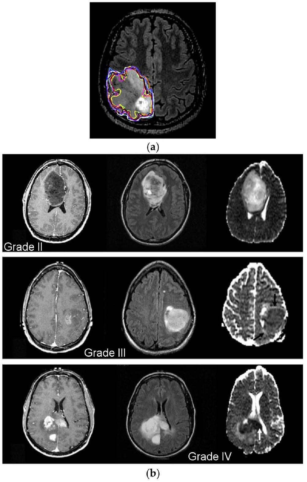
الشكل 1 أ تقسيم الورم يدويًا؛ درجة منظمة الصحة العالمية II (الصف الأول)، الدرجة III (الصف الثاني)، والدرجة IV (الصف الثالث) من أورام الدماغ
أحدث نموذج CNN يحتوي على ثلاثة خلايا عصبية في طبقة الإخراج لأنه مصمم لتقسيم كل صورة إلى ثلاث مجموعات. يتم إرسال الطبقة المتصلة بالكامل النهائية، والتي هي متجه ميزات ثلاثي الأبعاد، إلى مصنف softmax كمدخل. ثم يقوم مصنف softmax بإجراء تنبؤ نهائي حول درجة الورم. يوضح الجدول 4 معلومات مفصلة عن نموذج CNN.

تقييم مقياس الأداء

من الضروري تحليل أداء التصنيف في أبحاث تصنيف الصور لتوفير أساس منطقي لنتائج التحقيق. تم استخدام العديد من
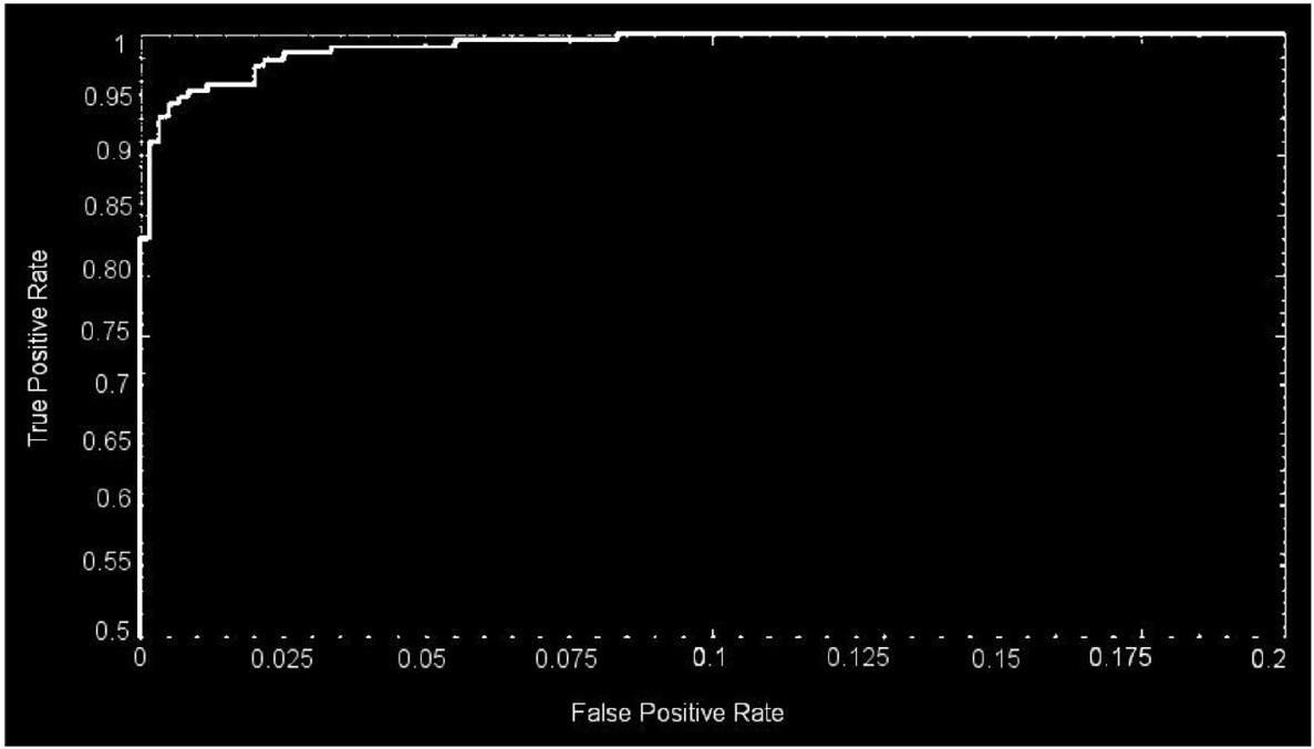
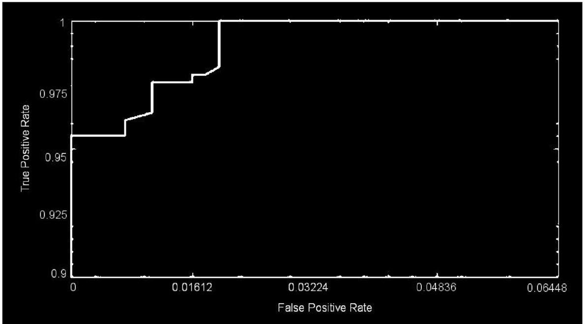
مقاييس تقييم الأداء المختلفة لفترة طويلة في الدراسات المتعلقة بتصنيف الصور والتي تطورت إلى مقاييس تقييم أداء قياسية في الدراسات المماثلة السابقة. استخدم النموذج المقترح طرقًا بارامترية مختلفة للتقييم، مثل الدقة، الحساسية، والدقة. تُعتبر هذه القياسات، التي تُعترف عمومًا كمقاييس تقييم أداء قياسية في أبحاث تصنيف الصور، مستخدمة أيضًا في هذه المقالة لقياس دقة وموثوقية عملية التصنيف. علاوة على ذلك، يتم استخدام منطقة منحنى التشغيل المستقبلي (ROC)، والمعروفة أيضًا باسم AUC من ROC
الجدول 1 عدد صور MRI في مجموعة البيانات
تقسيم مجموعة البيانات
تصنيف عدد الصور في المجموعة
النمط المجموعة إجمالي عدد الصور
1 خبيث 1743 3165
غير خبيث 1422
II حميد 910 4195
أورام دبقية 985
أورام سحائية 750
أورام نخامية 750
نقيلي 800
III G-II 1712 4720
G-III 1296
G-IV 1712
المنحنى، يُستخدم لتقييم أداء النماذج. فيما يلي المعادلات التي تحتوي على الصيغ المقابلة لكل من هذه القياسات:
حيث هو إيجابي حقيقي، هو سلبي حقيقي، هو إيجابي زائف، و هو سلبي زائف.

دراسة تجريبية

قمنا بتنفيذ نموذج التصنيف المقترح في MATLAB2021a على جهاز كمبيوتر بمواصفات 32 جيجابايت من الذاكرة العشوائية ومعالج Intel E3-1245v6 @3.70GHz.

تحسين المعلمات الفائقة

كانت هناك العديد من التطورات في مجال معالجة الصور الطبية التي أدت إلى زيادة استخدام CNNs، ونتيجة لذلك، ظهرت بعض التحديات في استخدامها. التصميمات المصممة للحصول على نتائج أكثر فعالية هي أعمق، وتصبح الصور المدخلة ذات جودة أعلى، مما يؤدي إلى زيادة في كمية الموارد المعالجة المطلوبة. تعتبر الأجهزة الكافية وضبط المعلمات الفائقة للشبكة ضرورية لتقليل هذه التكاليف الحاسوبية وتعظيم النتائج. نتيجة لذلك، تم ضبط جميع المعلمات الفائقة الأساسية لنماذج CNN المقترحة تقريبًا تلقائيًا باستخدام تقنية تحسين البحث الشبكي. عندما يكون مجال البحث عن القيم الممكنة صغيرًا، فإن تحسين البحث الشبكي هو وسيلة رائعة لتحسين تحسينات المعلمات الفائقة لـ CNN. يمكن أن يختار البحث الشبكي الأفضل من خلال تدريب الشبكة عبر مجموعة واسعة من التركيبات الممكنة. تحتوي نماذج CNN على هياكل معقدة جدًا ولديها الكثير من المعلمات الفائقة. في معظم الحالات، يمكن أن تكون هذه المعلمات الفائقة
الشكل 2 بنية نموذج CNN المقترح لنمط “C -1”
الجدول 2 معلومات مفصلة عن نموذج CNN المستخدم لنمط “C-1”
اسم الطبقة طبقة CNN التنشيطات المعلمات (قابلة للتدريب) إجمالي عدد المعلمات القابلة للتدريب
إدخال لا شيء 0
تلافيفية 128 ( )، خطوة (4،4)، مع حشو (0 00 0) أوزان، انحياز 13,954
طبقة تنشيط طبقة تنشيط-1 لا شيء 0
تطبيع تطبيع (عبر القناة) لا شيء 0
تجميع أقصى ( ) مع خطوة (2،2)، وحشو (000) لا شيء 0
تلافيفية 96 ( )، خطوة (1،1)، وحشو (2 22 2) أوزان، انحياز 49,246
طبقة تنشيط طبقة التفعيل-2 لا شيء 0
التجميع الأقصى ( بخطوة (2,2) وت padding (0 00 0) صفر 0
متصل بالكامل 512 متصل بالكامل أوزان تحيز 11,060,714
التسرب الدراسي 30٪ صفر 0
متصل بالكامل 2 متصل بالكامل أوزان تحيز ١٠٢٦
سوفتماكس سوفتماكس صفر 0
تصنيف ورم أو غير ورم لا شيء صفر 0
الشكل 3 هيكل نموذج CNN المقترح لوضع “C -2”
تنظم إلى فئتين متميزتين: المعلمات المعمارية والمعلمات الدقيقة للتعديل. تشمل المعلمات المعمارية ما يلي: عدد طبقات التجميع التلافيفي، عدد الطبقات المتصلة بالكامل، عدد المرشحات، المرشح
الأحجام، ودالة التفعيل. تعتبر تنظيم البيانات، والزخم، وحجم الدفعة الصغيرة، ومعدل التعلم من المعلمات الفائقة التي يتم ضبطها بدقة. في التحليل الحالي، يتم ضبط المعلمات الفائقة للهيكل في البداية باستخدام الخوارزمية 1.
الجدول 3 معلومات مفصلة عن نموذج CNN المستخدم في وضع “C-2”
اسم الطبقة طبقة CNN تفعيلات المعلمات (قابلة للتدريب) إجمالي عدد المعلمات القابلة للتدريب
مدخل صفر 0
التلافيفي خطوة (4,4) مع حشو (0 00 0) أوزان تحيز ١٣,٩٥٢
طبقة التفعيل طبقة التفعيل – 1 صفر 0
التطبيع التطبيع (عبر القنوات) لا شيء 0
التجميع الأقصى بخطوة من ، و ( 000 ) حشو صفر 0
التلافيفي ٩٦ خطوة (1,1) ووسادة (2 22 2) أوزان تحيز ٤٤٢,٤٦٤
طبقة التفعيل طبقة التفعيل-2 صفر 0
التجميع الأقصى ( بخطوة (2,2) و padding (000) صفر 0
التلافيفي ٩٦ الخطوة (1,1) و (222 2) الحشو أوزان تحيز ٣٦,٩٦٠
طبقة التفعيل طبقة التفعيل – 3 لا شيء 0
التجميع الأقصى ( ) بخطوة ( 2,2 )، و ( 000 ) حشو صفر 0
التلافيفي ٢٤ ( خطوة (1,1) و(222 2) حشوة أوزان تحيز 82,968
طبقة التفعيل طبقة التفعيل-4 صفر 0
التجميع الأقصى ( ) بخطوة ( 2,2 ) و ( 000 ) حشو لا شيء 0
التلافيفي 24 ( خطوة (1,1) و (222 2) حشوة أوزان تحيز ٢٠٧٦٠
طبقة التفعيل طبقة التفعيل-5 صفر 0
التجميع الأقصى ( بخطوة (2,2) و padding (000) صفر 0
التلافيفي خطوة (1,1) وت padding (2222) أوزان تحيز ١٢٣٢٠
طبقة التفعيل طبقة التفعيل-6 لا شيء 0
التجميع الأقصى ( بخطوة (2,2) و padding (000) لا شيء 0
متصل بالكامل 512 متصل بالكامل أوزان تحيز 16,896
التسرب الدراسي 30٪ لا شيء 0
متصل بالكامل 5 متصل بالكامل أوزان تحيز 2565
سوفتماكس سوفتماكس لا شيء 0
تصنيف حميد، ورم دبقي، ورم غدي، ورم نقوي، وورم سحائي صفر لا شيء 0
الخوارزمية 1. سيتم تحسين المعلمات المعمارية باستخدام خوارزمية البحث الشبكي
ابدأ
الخطوة 1: تخصيص شبكة ذات 5 أبعاد للمعلمات الخمسة التي تحتاج إلى تحسين.
الخطوة 2: يجب تعيين فترات القيم المحتملة لكل بُعد.
– طبقات التجميع الأقصى والتلافيف = (1,2,3,4)
الخطوة 3: افحص جميع التوليفات المحتملة واختر تلك التي تعظم الدقة العامة.
دقة
نهاية
بعد تحديد المعلمات المعمارية، يتم استخدام الخوارزمية 2 لتحسين معلمات الضبط الدقيق. في هذه الدراسة المقترحة، يتم إجراء بحث شبكي على مجموعة التدريب باستخدام طريقة التحقق المتقاطع بخمس طيات. يتم تقسيم مجموعة البيانات إلى خمس مجموعات مختلفة. تُستخدم أربع من هذه المجموعات للتدريب، وتُستخدم المجموعة الخامسة للاختبار. بالنسبة لوضع التصنيف 1، هناك 3165 صورة، وبالنسبة لوضع التصنيف 2، هناك 4195 صورة، وبالنسبة لوضع التصنيف 3، هناك 4720 صورة. لكل وضع تصنيف، يتم تقسيم مجموعة البيانات عشوائيًا إلى مجموعة تدريب، مجموعة تحقق، ومجموعة اختبار، بنسبة 60:20:20. بشكل أساسي، تمر طريقة البحث الشبكي عبر كل إعداد ممكن لكل معلمة وتجد الإعداد الذي يعطي أفضل أداء. من أجل الحصول على أعلى درجة ممكنة من الدقة مع الخوارزمية 1، هناك خمس معلمات تحتاج إلى تحسين.
الشكل 4 نموذج العمارة المقترح لشبكة CNN لوضع “C -3”
الخوارزمية 2. سيتم تحسين المعلمات المعمارية باستخدام خوارزمية البحث الشبكي
Begin
Step 1: Assign a 4-dimensional grid for the 5 hyperparameters needed to be optimized.
- Regularization = R2
- A momentum
- Size of the minibatches
- Rate of learning
Step 2: To each dimension, potential value intervals should be assigned.
- R2 = (0.0002, 0.00043, 0.002, 0.004)
- A momentum = (0.78, 0.77, 0.954, and 0.96)
- Size of the minibatches = (4,6, 16, 24, 32, 64)
- Rate of learning = (0.0002, 0.00043, 0.002, 0.004)
Step 3: Examine all the potential pairings and choose the one that maximizes overall ac-
curacy.
- A1 = (0.0002, 16, 0.16, 0.0002) }->mathrm{ accuracy 94.6%
- A2 = (0.0005, 32, 0.9, 0.002) }->mathrm{ accuracy }98.4
- A3 = (0.0002, 64, 0.9, 0.002) }->mathrm{ accuracy }99.2
End
العديد من التركيبات الممكنة لهذه المعلمات، بما في ذلك ، و 4 ، على التوالي. ونتيجة لذلك، فإن العدد الإجمالي للتباديل الممكنة التي سيتم فحصها هو ، مما يعادل 2240. نظرًا لأن 2240 تركيبة تحتاج إلى التحقق منها باستخدام تقنية التحقق المتقاطع الخماسي، يتم تنفيذ خوارزمية البحث الشبكي التي تم إنشاؤها لتحسين معلمات نموذج الشبكة العصبية التلافيفية 11,200 مرة. مشابهة للخوارزمية الأولى، تحتوي الخوارزمية الثانية على أربعة معلمات تحتاج إلى تحسين لتحقيق أعلى مستوى من الدقة. هناك مجموعة واسعة من التباديل الممكنة في هذه المعلمات،
على سبيل المثال، “، و 4. ونتيجة لذلك، فإن العدد الإجمالي للتباديل الممكنة التي يجب فحصها هو ، مما يعادل 320. نظرًا لأن هناك 320 مجموعة ممكنة مختلفة تحتاج إلى اختبار باستخدام طريقة التحقق المتقاطع بخمسة أضعاف، يتم تنفيذ تقنية البحث الشبكي التي تم تطويرها لتحسين تصحيح المعلمات الفائقة لنموذج CNN بمجموع 1600 مرة. كما هو موضح في الجداول 5 و 6 و 7، وجد خوارزمية تحسين البحث الشبكي أفضل القيم الممكنة للمعلمات الفائقة لوضعيات C-1 و C-2 و C-3.

نتائج الشبكة العصبية التلافيفية المحسّنة

يتم استخدام نهج التحقق المتقاطع بخمسة أضعاف لنمط C-1 لإجراء تحليل أداء النموذج المقترح. يتم تقسيم مجموعة البيانات إلى خمس مجموعات مختلفة، يتم استخدام أربع منها لأغراض التدريب، بينما يتم استخدام المجموعة الخامسة لأغراض الاختبار. هناك خمس تكرارات إجمالية للتجارب، ويتم تقييم أداء التصنيف للنمط في كل طية، ثم يتم حساب متوسط أداء التصنيف العام للنموذج. إن النتائج العالية من دورتَي التدريب والتحقق غير ذات معنى إذا لم يتم اختبار الشبكة العصبية التلافيفية المدربة والمضبوطة على قدرتها على التنبؤ بعينات لم تُرَ من قبل. لذلك، لتقييم فعالية الشبكة العصبية التلافيفية المدربة.
الجدول 4 معلومات مفصلة عن نموذج CNN المستخدم في وضع “C-3”
اسم الطبقة طبقة CNN التفعيل المعلمات (قابلة للتدريب) إجمالي عدد المعلمات القابلة للتدريب
مدخل صفر 0
التلافيفي 128 ( خطوة (4,4)، مع حشو (0 00 0) أوزان تحيز ١٣,٩٥٢
طبقة التفعيل طبقة التفعيل – 1 صفر 0
التطبيع التطبيع (عبر القنوات) صفر 0
التجميع الأقصى ( ) بخطوة ( 2,2 ) و ( 000 ) حشو صفر 0
التلافيفي ٩٦ ( خطوة (1,1) ووسادة (2 22 2) أوزان تحيز ٤٦,٧٥٢
طبقة التفعيل طبقة التفعيل-2 صفر 0
التجميع الأقصى ( ) بخطوة ( 2,2 )، و ( 000 ) حشو صفر 0
التلافيفي ٩٦ ( خطوة (1,1) و(222 2) حشوة أوزان تحيز ٣٦,٨٦٤
طبقة التفعيل طبقة التفعيل-3 صفر 0
التجميع الأقصى ( بخطوة (2,2) وت padding (0 00 0) صفر 0
متصل بالكامل 512 متصل بالكامل أوزان تحيز 3,146,240
التسرب الدراسي 30٪ صفر 0
متصل بالكامل 3 متصل بالكامل أوزان تحيز 1539
سوفتماكس سوفتماكس صفر 0
تصنيف جي-2، جي-3، جي-4 صفر صفر 0
تكون فعالية شبكة CNN في التنبؤ بالعينات، حيث يتم تخصيص مجموعة بيانات اختبار بشكل عشوائي وفصلها جنبًا إلى جنب مع مجموعات بيانات التدريب والتحقق. إذا تم تخطي هذه الخطوة، فقد تؤدي الدقة العالية إلى نتيجة ناتجة عن تخصيص مجموعة بيانات متحيزة. تعرض الجدول 8 نتائج تقسيم 3165 صورة من الدراسة بشكل عشوائي إلى مجموعات التدريب والتحقق والاختبار بنسبة 60:20:20 لوضع C-1.
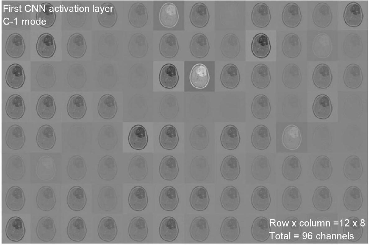
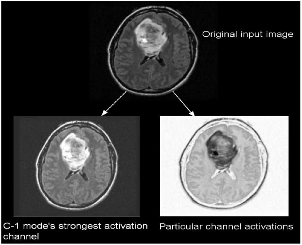
تم أخذ ما مجموعه 299 صورة بشكل عشوائي من مجموعة البيانات لكل فئة، ثم تُستخدم تلك الصور للاختبار. يمكن عرض تنشيطات طبقات الالتفاف في الشبكة العصبية التلافيفية للحصول على رؤية أفضل للميزات.
الجدول 5 النتائج المثلى التي تم الحصول عليها من البحث الشبكي للمعلمات الفائقة لوضع C-1
الهايبر بارامترز تغييرات في قيم المعلمات القيمة القصوى
طبقات التجميع الأقصى والشبكات العصبية التلافيفية (1، 2، 3، 4) 2
عدد الطبقات المتصلة بالكامل (1، 2، 3، 4) ٢
إجمالي عدد الفلاتر (8، 16، 24، 32، 48، 64، 96، 128، 256) ٦٤، ٩٦، ١٢٨
شدة الترشيح (3، 4، 5، 6، 7) 6,6
دور التنشيط (ريلو، إيلو، ريليو المتسرب) ريلو
حجم الدفعة الصغيرة (٤، ٦، ١٦، ٢٤، ٣٢، ٦٤) 32
معدل التغير (0.78، 0.77، 0.95، 0.96) 0.95
معدل التعلم (0.0002, 0.00043, 0.002, 0.004) 0.0002
-تنظيم (0.0002، 0.00043، 0.002، 0.004) 0.0002
أن CNN قد تعلمت بسبب تدريبها. مع هذا التمثيل، يمكن للباحث بسهولة ملاحظة تقدم الشبكة. الأشكال 5 و 6 كل منهما تصور تنشيطات الطبقات التلافيفية الأولى والثانية. واحدة من الصور في الشبكة تمثل نتيجة القناة. تمثل المناطق البيضاء تنشيطات إيجابية عالية، بينما تمثل المناطق الرمادية قنوات نشطة بشكل معتدل. بينما تُستخدم الطبقة التلافيفية الأولى من CNN لتعلم ميزات مثل اللون والحواف، تُستخدم الطبقة التلافيفية الثانية لتعلم معلومات أكثر تعقيدًا، مثل حدود أورام الدماغ. الطبقات التلافيفية التالية (الأعمق)
الجدول 7 النتائج المثلى التي تم الحصول عليها من خلال البحث الشبكي للمعلمات الفائقة لنموذج C-3
الهايبر بارامترز تغييرات في قيم المعلمات القيمة القصوى
طبقات التجميع الأقصى والشبكات العصبية التلافيفية (1، 2، 3، 4) ٣
عدد الطبقات المتصلة بالكامل (1، 2، 3، 4) 2
إجمالي عدد الفلاتر (8، 16، 24، 32، 48، 64، 96، 128، 256) ٦٤، ٩٦، ١٢٨
شدة الترشيح (3، 4، 5، 6، 7) ٦، ٦، ٤
دور التنشيط (ريلو، إيلو، ريليو المتسرب) ريلو
حجم الدفعة الصغيرة (٤، ٦، ١٦، ٢٤، ٣٢، ٦٤) 32
معدل التغير (0.78، 0.77، 0.95، 0.96) 0.95
معدل التعلم (0.0002, 0.00043, 0.002, 0.004) 0.004
-تنظيم (0.0002، 0.00043، 0.002، 0.004) 0.002
الجدول 6 النتائج المثلى التي تم الحصول عليها من البحث الشبكي للمعلمات الفائقة لوضع C-2
الهايبر بارامترز تغييرات في قيم المعلمات القيمة القصوى
طبقات التجميع الأقصى والشبكات العصبية التلافيفية (1، 2، 3، 4) ٦
عدد الطبقات المتصلة بالكامل (1، 2، 3، 4) 2
إجمالي عدد الفلاتر (8، 16، 24، 32، 48، 64، 96، 128، 256) 16، 24، 32، 48، 64، 96، 128
شدة الترشيح (3، 4، 5، 6، 7) ٦، ٦، ٤، ٦، ٢، ٦
دور التنشيط (ريلو، إيلو، ريليو المتسرب) ريلو
حجم الدفعة الصغيرة (٤، ٦، ١٦، ٢٤، ٣٢، ٦٤) 64
معدل التغير (0.78، 0.77، 0.95، 0.96) 0.95
معدل التعلم (0.0002، 0.00043، 0.002، 0.004) 0.0002
-تنظيم (0.0002, 0.00043, 0.002, 0.004) 0.002
يبنون ميزاتهم من خلال دمج الميزات التي تم تعلمها بواسطة الطبقات التلافيفية السابقة.
تظهر الشكل 5 96 من 128 قناة في الطبقة التلافيفية الأولى لشبكة CNN تعمل في وضع C-1. تحتوي هذه الطبقة على إجمالي 128 قناة. يظهر الشكل 6 صورة للطبقة التلافيفية الثانية للشبكة، التي تحتوي على 96 قناة. كل طبقة من شبكة CNN تتكون من قنوات، وهي مصفوفات في بعدين. تمثل إحدى الصور في الشكل 5 مخرجات كل قناة في الطبقة التلافيفية الأولى. في هذه الصور، تُظهر البكسلات البيضاء تنشيطات إيجابية قوية، بينما تُظهر البكسلات السوداء تنشيطات سلبية قوية. وبالمثل، تشير البكسلات الرمادية في الصورة المدخلة إلى قنوات ليست نشطة بشكل كبير. يوضح الشكل 7 تنشيطات قناة معينة والقناة ذات التنشيط الأكثر أهمية في الطبقة التلافيفية الأولى. وجود البكسلات البيضاء في قناة الشكل 7 يدل على أن هذه القناة نشطة بشكل كبير في موقع الورم. على الرغم من أن شبكة CNN لم تُعطَ تعليمات لتعلم حول الأورام، إلا أنه من الممكن الاستنتاج أنها قد التقطت حقيقة أن الأورام لها خصائص مميزة تسمح لها بالتفريق بين فئات مختلفة من الصور.
تستطيع هذه الشبكات العصبية التلافيفية اكتشاف الخصائص المفيدة بمفردها، على عكس طرق الشبكات العصبية الاصطناعية السابقة التي كانت تتطلب عادةً تصميمًا يدويًا لتناسب نمطًا معينًا. في هذه المقالة المقترحة، يُحسن التعلم للتعرف على الأورام القدرة على التمييز بين صورة ورم وصورة غير ورم. بعد الانتهاء من عملية التصنيف، يجب تقييم كفاءة نماذج الشبكات العصبية التلافيفية باستخدام طرق موثوقة مختلفة. تُستخدم مقاييس مثل الخصوصية والحساسية والدقة وقياسات الدقة، بالإضافة إلى المساحة تحت منحنى ROC، لإجراء تقييم الأداء للنموذج المقترح. تُظهر الرسوم البيانية لفقدان ودقة الشبكة العصبية التلافيفية المقترحة لنمط C-1 في الشكل 8. بعد 340 تكرارًا، كان النموذج المقترح لنمط C-1 قادرًا على التصنيف بـ الدقة. من الواضح، كما هو موضح في الشكل 8، أن حوالي 250 تكرارًا مطلوبة للوصول إلى مستوى دقة شبه مثالي. الشكل 9 يوضح مصفوفة الالتباس لوضع التصنيف-1. كما يمكن رؤيته في الشكل 10، فإن المساحة تحت منحنى ROC لها قيمة 0.9995 لمقياس AUC. النتائج المقدمة هنا تظهر أن نموذج CNN الموصى به قادر على تحديد أورام الدماغ. الجدول 9 يعرض مقاييس
الجدول 8 مراحل التدريب والتحقق والاختبار لنموذج CNN المقترح
تقسيم مجموعة البيانات أوضاع التدريب والتحقق والاختبار
تصنيف عدد الصور في المجموعة إجمالي عدد الصور وضع التدريب (60%) وضع التحقق (20%) وضع الاختبار (20%)
1 خبيث 1743 3165 1899 ٦٣٣ ٦٣٣
غير خبيث 1422
الثاني حميد 910 ٤١٩٥ ٢٥١٧ 839 839
ورم دبقي 985
ورم السحايا 750
الغدة النخامية 750
نقيلية ٨٠٠
ثالث جي-2 1712 4720 ٢٨٣٢ 944 944
جي-ثري ١٢٩٦
جي-4 1712
الشكل 5 أول طبقة تفعيل لشبكة CNN لوضع C-1
الشكل 6 الطبقة الثانية لتفعيل الشبكة العصبية التلافيفية لنمط C-1
الدقة، مثل الإيجابيات الحقيقية (TP)، السلبيات الحقيقية (TN)، الإيجابيات الكاذبة (FP)، السلبيات الكاذبة (FN)، الدقة (Acc)، الخصوصية (Sp)، الحساسية (Se)، والدقة (Pr). الشكل 10 يوضح منحنى ROC لمهمة التصنيف-1 (C-1).
تظهر الشكل 11 نتائج التصنيف والاحتمالات المتوقعة لكل من الاختبارات الأربعة التي أجريت في وضع C-1. تم تنفيذ طريقة التحقق المتقاطع بخمسة أضعاف لـ تقوم الوضعية بتقييم فعالية الإطار المقترح. يتم تقسيم مجموعة البيانات إلى خمس مجموعات، يتم استخدام أربع منها.
لأغراض التدريب، بينما يتم تخصيص المجموعة الخامسة لأغراض الاختبار. هناك خمس تكرارات إجمالية للتجارب. يتم تقييم أداء التصنيف للوظيفة لكل طية، ثم يتم حساب متوسط أداء التصنيف العام للنموذج. كما هو موضح في الجدول 8، هناك صور كافية لـ -وضع التدريب، والتحقق، ومجموعات الاختبار لتقسيمها عشوائيًا بنسبة لعينة حجمها 4195. من مجموعة البيانات لكل فئة التي ستستخدم لاختبار النموذج، يتم اختيار 158 صورة عشوائيًا لإزالتها. تمثيلات الدقة والخسارة للنموذج المقترح لشبكة CNN لـ
الشكل 7 صور الوضع C-1 الأقوى والمتوسطة من الصورة المدخلة الأصلية
الشكل 8 منحنيات دقة وضع C-1 وخسارة
تظهر مهام C-2 في الشكل 12. الطريقة المقترحة للشبكة العصبية التلافيفية (CNN) لنمط C-2 تحقق دقة تبلغ 93.81% في التصنيف بعد 294 تكرارًا. كما هو موضح في الشكل 13، فإن المساحة تحت منحنى ROC لها قيمة تبلغ 0.9981. هذه النتائج توضح قدرة نموذج CNN المقترح على تصنيف أنواع أورام الدماغ. الشكل 14 يصور مصفوفة الالتباس، والجدول 9 يسرد العديد من مقاييس الدقة، مثل TP وTN وFP وFN وAcc وSp وSe وPr. وفقًا للجدول 9، فإن الدقة تبلغ يتم تحقيقه عند تصنيف الورم الدبقي، عند تصنيف ورم السحايا، عند تصنيف النقائل، عند تصنيف الدماغ الصحي، و عند تصنيف نوع ورم الغدة النخامية لنمط C-2.
تظهر الشكل 14 منحنى ROC لمهمة التصنيف-2 (C-2).
تُستخدم عملية التحقق المتقاطع الخماسي لتقييم فعالية النماذج المقترحة في وضع C-3. يتم تقسيم مجموعة البيانات إلى خمس مجموعات مختلفة، حيث تُستخدم أربع منها للتدريب والخامسة للاختبار. هناك خمس تكرارات إجمالية للتجارب. بعد تحليل أداء التصنيف للوضع لكل مجموعة، يتم حساب متوسط أداء التصنيف للنموذج. بالنسبة لوضع C-3، يمكن تقسيم الصور الكافية عشوائيًا إلى مجموعات التدريب والتحقق والاختبار بالنسب 60:20:20، كما هو موضح في الجدول 8، مع استبعاد ثلاثمائة صورة عشوائيًا.
فئة الهدف
غير ورمي 268 44.9% 3 0.6% 98.72% 1.28%
فئة الإخراج ورم 0 0.0% 326 54.1% 100% 0.0%
100% 0.0% 98.9% 1.1% 99.5% 0.6%
ورم غير ورمي إجمالي
الشكل 9 مصفوفة الالتباس C-1
الشكل 10 متوسط وضع C-1 لمنحنى ROC
وخمس صور من مجموعة البيانات لكل فئة سيتم استخدامها لتقييم النموذج. تُظهر الرسوم البيانية للخسارة والدقة لشبكة CNN المقترحة لوضع C-3 في الشكل 15. يوضح الشكل 16 مصفوفة الالتباس لوضع C-3. تحصل الطريقة المقترحة لوضع C-3 على دقة تصنيف قدرها بعد 344 تكرارًا. الشكل 17 يوضح منحنى ROC لمهمة التصنيف-3 (C-3). الجدول 9 يظهر أن الدقة تبلغ يتم الوصول إليه عند تصنيف الدرجة الثانية، متى
تصنيف الدرجة الثالثة، و عند تصنيف الدرجة الرابعة لأورام الدماغ في وضع C-3. تم مقارنة النتائج الثلاثة المختلفة لتصنيف نموذج الشبكة العصبية الالتفافية المقترح مع نتائج طرق الشبكة العصبية الالتفافية التقليدية الأخرى لتقييم قدرة تصنيف النظام المقترح. لتحقيق هذا الهدف، تم إجراء نفس التجارب باستخدام نفس مجموعة البيانات، مع الاستفادة من نماذج الشبكة العصبية الالتفافية المدربة مسبقًا المعروفة والشائعة، مثل AlexNet وDenseNet121 وResNet-101 وVGG-16، و
الجدول 9 نتائج مقاييس معلمات نموذج CNN المقترح لجميع أوضاع التصنيف
المقاييس فصول تي بي TN FP FN حساب سب سي بر إجمالي
1 خبيث ٢٦٨ ٣٢٦ ٣ 0 99.50 99.09 100.00 98.89 ٢٦٨
غير خبيث ٣٢٦ ٢٦٨ 0 ٣ 99.50 100.00 99.09 100.00 ٣٢٩
الثاني حميد 183 598 ٨ ٨ 97.99 98.68 95.81 95.81 191
ورم دبقي 132 ٦٥٠ 10 12 97.26 ٩٨.٤٨ 91.67 92.96 ١٤٤
ورم السحايا 138 643 ٦ 14 ٩٧.٥٠ 99.08 90.79 95.83 152
الغدة النخامية ١٦٠ 598 ٢٤ 11 95.59 ٩٦.١٤ 93.57 ٨٦.٩٦ 171
نقيلية 127 643 11 14 ٩٦.٨٦ ٩٨.٣٢ 90.07 92.03 141
ثالثاً جي-2 ٣٣٢ 574 9 ٨ 98.16 ٩٨.٤٦ ٩٧.٦٥ ٩٧.٣٦ ٣٤٠
جي-ثري ٢٤٨ 679 0 0 100.00 100.00 100.00 100.00 ٢٤٨
جي-4 ٣٣٠ 580 ٨ 9 ٩٨.١٧ ٩٨.٦٤ ٩٧.٣٥ ٩٧.٦٣ ٣٣٩
الشكل 11 نتائج التصنيف والتنبؤات لاحتمالات أربع صور اختبار مختلفة لوضع C-1
الشكل 12 منحنيات دقة وضع C-2 والخسارة
الشكل 13 متوسط وضع C-2 لمنحنى ROC
فئة الهدف
ورم دبقي 183 ٣ ٤ 1 0 95.9%
٢٢.٨٪ 0.4% 0.5% 0.1% 0.0% ٤.١٪
ورم السحايا ٤ 132 ٣ 1 2 93.8٪
0.5% 16.3% 0.4% 0.1% 0.3% 6.2%
فئة الإخراج نقيلية 1 2 138 ٢ 1 95.9٪
0.1% 0.3% 17.4% 0.3% 0.1% ٤.١٪
حميد ٣ ٤ ٦ ١٦٠ 11 86.8%
0.4% 0.5% 0.8% ٢٠.٢٪ 1.4٪ 13.2%
الغدة النخامية 0 ٣ 1 ٧ 127 93.1٪
0.0% 0.4% 0.1% 0.9% 15.9% 6.9%
95.3٪ 93.9٪ 92.7% 93.6٪ 90.0% 93.8%
٤.٧٪ 6.1٪ ٧.٣٪ 6.4% 10.0% 6.9%
ورم دبقي ورم السحايا نقيلية حميد الغدة النخامية إجمالي
الشكل 14 مصفوفة الارتباك C-2
جوجل نت. توضح الجدول 10 مقارنة نتائج مقاييس الأداء للنموذج المقترح من CNN مع الأساليب الحالية لـ CNN. تُظهر الشكل 18 التمثيل البياني لمقارنة نتائج النماذج المقترحة والحالية.
توضح النتائج المعروضة في الجدول 10 أن نماذج CNN المقترحة تتفوق على الشبكات الأخرى في كل وضع تصنيف. تم تدريب DenseNet121 مسبقًا
نموذج، الذي يحصل على دقة التصنيف في اختبار كشف أورام الدماغ الوضع)، هو النموذج الأقرب إلى النموذج المقترح. يحصل نموذج VGG-16 المدرب مسبقًا على الدقة في وضع تصنيف نوع ورم الدماغ (وضع C-2). إنه النموذج الأقرب إلى نموذج CNN المقترح. بعد نموذج CNN المقترح، يحقق نموذج GoogleNet المدرب مسبقًا دقة تصنيف تبلغ
الشكل 15 منحنيات دقة وضع C-3 وخسارة
فئة الهدف
جي 332 37.2% 0 0.0% 9 1.1% 97.7% 2.3%
فئة الإخراج
0 0.0% 248 26.1% 0 0.0% 100% 0.0%
هو 8 0.8% 0 0.0% ٣٣٠ ٣٥.١٪ 98.1% 1.9%
100% 0.0% 97.5% 2.5% 98.1% 1.9% 98.5% 1.5%
مؤشر الابتكار العالمي جي 3 جيف إجمالي
الشكل 16 مصفوفة الارتباك C-3
95.12%، مما يجعلها أفضل شبكة متاحة لتصنيف الأورام (وضع C-3). من الواضح أن نماذج CNN المقترحة أفضل من الشبكات المدربة مسبقًا، التي تم بناؤها وتدريبها باستخدام مجموعات بيانات وأساليب عامة لمجموعة واسعة من مهام تصنيف الصور. توضح الجدول 11 مقارنة نتائج النماذج المقترحة والحالية. تم تصميم نماذج CNN المقترحة، على العكس، للتعامل مع قضايا أكثر تحديدًا، مثل تحديد وتعريف أنواع ومراحل مختلفة من أورام الدماغ. أخيرًا، تُستخدم صور الرنين المغناطيسي لأورام الدماغ لتدريب وتقييم النماذج المقترحة.

الاستنتاجات

في هذا البحث، نقترح طريقة تصنيف متعددة لتحديد أورام الدماغ في مرحلة مبكرة باستخدام نماذج الشبكات العصبية التلافيفية (CNN)، حيث يتم تحسين جميع المعلمات الفائقة تقريبًا تلقائيًا من خلال البحث الشبكي. من خلال استخدام مجموعات بيانات التصوير الطبي المتاحة للجمهور، تم تخصيص ثلاثة نماذج CNN موثوقة لأداء ثلاث مهام تصنيف أورام الدماغ متميزة. مستوى عالٍ من الدقة، مثل يمكن تحقيقه في عملية اكتشاف أورام الدماغ. بالإضافة إلى ذلك، دقة ملحوظة من يتم تحقيقه
الشكل 17 متوسط وضع C-3 لمنحنى ROC
الجدول 10 مقارنة نتائج مقاييس الأداء للنموذج المقترح لشبكة CNN مع الأساليب الحالية لشبكات CNN
نماذج سي إن إن وضع C-1 وضع C-2 وضع C-3
الدقة (%) الجامعة الأمريكية في القاهرة الدقة (%) الجامعة الأمريكية في القاهرة الدقة (%) الجامعة الأمريكية في القاهرة
جوجل نت ٧٤.٢١ 0.8108 ٧٧.٨٩ 0.8212 95.12 0.9617
أليكس نت 89.23 0.8989 84.24 0.8501 91.08 0.9772
دينس نت 121 93.89 0.9412 ٧٧.٦٧ 0.8122 ٨٦.٠٧ 0.8809
ريسنت101 93.29 0.9442 ٧٦.٤٥ 0.8115 ٨٦.٤٢ 0.881
في جي جي – 16 ٨٨.٨٧ 0.9201 ٨٩.١٩ 0.8112 84.87 0.8663
النهج المقترح لشبكة CNN 99.53 0.9994 93.81 0.9984 ٩٨.٥٦ 0.9993
الشكل 18 توضيح بياني لمقارنة نتائج النماذج المقترحة وال existentes
الجدول 11 مقارنة بين النموذج المقترح والدراسات الحالية
مؤلف سنة مجموعات البيانات طريقة تصنيف الدقة (%)
أحمد واصف رضا [12] ٢٠٢٣ كاجل، فيغشير معمارية VGG-16 ٩٦.٧٠
محمود خالد عبد الله [13] 2018 رايدر، رمبرانت، وبرايتس إيكوك-إس في إم ٩٧.٩٨
تاكوا رحمن [27] ٢٠٢٣ كاجل، ريمبرانت سي إن إن + 6 نماذج مدربة مسبقًا 97.12
أناند ديشباندي [17] ٢٠٢١ رايدر وبرايتس دمج الصور المعتمد على تحويل كوساين المتقطع مع الشبكات العصبية التلافيفية ٩٨.١٤
النموذج المقترح ٢٠٢٣ فيغشير، ريمبراندت، TCGA-LGG، TCIA شبكة عصبية تلافيفية هجينة ٩٨.٥٦
عند تصنيف صور الرنين المغناطيسي للدماغ إلى فئات الورم الدبقي، والورم السحائي، والغدة النخامية، والدماغ الطبيعي، والورم النقوي. الخطوة النهائية هي تصنيف أورام الدماغ الدبقية، والتي يمكن أن تتم بدقة تبلغ للمستويات الثانية والثالثة والرابعة. يتم استخدام عدد جيد من الصور الطبية لتدريب واختبار نماذج الشبكات العصبية التلافيفية (CNN) المقترحة. تظهر النتائج من نماذج CNN المقترحة والمقارنات مع الطرق الحالية أن نماذج CNN المصنوعة بإطار العمل الأمثل المقترح تعمل بشكل جيد. في هذا العمل، تم إنشاء نماذج CNN يمكن أن تساعد الأطباء والمختصين في الأشعة في فحص الفحوصات الأولية لعدة أنواع من أورام الدماغ.

شكر وتقدير

غير قابل للتطبيق.

بيان لجنة المراجعة المؤسسية

غير قابل للتطبيق.

قائمة التحقق لأبحاث المشاركين البشريين:

أكمل ما يلي إذا كانت دراستك تتضمن مشاركين بشريين أو بيانات لمشاركين بشريين. يجب معالجة هذه الأسئلة للدراسات المستقبلية والاستعادية.
  1. هل حصلت على موافقة الأخلاقيات لهذه الدراسة؟
  • إذا كانت الإجابة نعم، يرجى رفع (نوع الملف “آخر”) الوثيقة الأصلية للموافقة التي تلقيتها من لجنة الأخلاقيات الخاصة بك. إذا كانت الوثيقة الأصلية بلغة أخرى، يرجى أيضًا تقديم ترجمة إلى الإنجليزية.
    الرد: غير متوفر
  • إذا لم تحصل على موافقة أخلاقية، يرجى توضيح سبب عدم الحاجة لذلك أدناه.
  1. إذا قمت بتجنيد مشاركين بشريين للدراسة على سبيل المثال، أجريت تجربة سريرية، وزعت استبيانات، أو حصلت على أنسجة أو بيانات أو عينات لأغراض هذه الدراسة، يرجى الإبلاغ في القسم الخاص بالطرق: i. اليوم والشهر والسنة لبداية ونهاية فترة التجنيد لهذه الدراسة.
    ii. ما إذا كان المشاركون قد قدموا موافقة مستنيرة، وإذا كان الأمر كذلك، ما نوعها (على سبيل المثال، مكتوبة أو شفهية، وإذا كانت شفهية، كيف تم توثيقها وشهادتها). إذا كانت دراستك تشمل قاصرين، يرجى بيان ما إذا كنت قد حصلت على موافقة من الوالدين أو الأوصياء. إذا تم التنازل عن الحاجة إلى الموافقة من قبل لجنة الأخلاقيات، يرجى تضمين هذه المعلومات.
    الرد: غير متوفر
  2. إذا كنت تقوم بتقديم دراسة استعادية لسجلات طبية أو عينات مؤرشفة، يرجى الإبلاغ في قسم الطرق:
    i. اليوم والشهر والسنة التي تم فيها الوصول إلى البيانات لأغراض البحث ii. ما إذا كان المؤلفون قد حصلوا على معلومات يمكن أن تحدد المشاركين الأفراد أثناء أو بعد جمع البيانات
    الرد: غير متوفر

مساهمات المؤلفين

تصور، س.س. و د.ف.; المنهجية، س.ك.م. و ح.ر.; التحقق، ح.ر. و م.أ.س.; تنظيم البيانات، ب.د.س.; كتابة – المسودة الأصلية، س.س. و د.ف.; كتابة – المراجعة والتحرير، س.ك.م. و ح.ر.; التصور، ب.د.س; الإشراف س.ك.م. و م.أ.س.; إدارة المشروع، س.ك.م. و م.أ.س. جميع المؤلفين قرأوا ووافقوا على النسخة المنشورة من المخطوطة.

تمويل

لم تتلقَ هذه الدراسة أي تمويل خارجي.

توفر البيانات والمواد

تتوفر مجموعات البيانات المستخدمة خلال الدراسة الحالية من المؤلف المراسل عند الطلب المعقول.

الإعلانات

غير قابل للتطبيق.

تنافس المصالح

يعلن المؤلفون عدم وجود مصالح متنافسة.
تاريخ الاستلام: 7 نوفمبر 2023 تاريخ القبول: 8 يناير 2024
نُشر على الإنترنت: 19 يناير 2024

References

  1. Abiwinanda N, Hanif M, Hesaputra ST, Handayani A, Mengko TR. Brain tumor classification using convolutional neural network. IFMBE Proc. 2019;68:183-9.
  2. Ayadi W, Elhamzi W, Charfi I, Atri M. Deep CNN for brain tumor classification. Neural Process Lett. 2021;53:671-700.
  3. Badža MM, Barjaktarović MČ. Classification of brain tumors from MRI images using a convolutional neural network. Appl Sci. 1999;2020:10.
  4. Saravanan S, Kumar VV, Sarveshwaran V, Indirajithu A, Elangovan D, Allayear SM. Computational and Mathematical Methods in Medicine Glioma Brain Tumor Detection and Classification Using Convolutional Neural Network. Comput Math Methods Med. 2022;2022:4380901.
  5. Ge C, Gu IYH, Jakola AS, Yang J. Deep semi-supervised learning for brain tumor classification. BMC Med Imaging. 2020;20:87.
  6. Cinar A, Yildirim M. Detection of tumors on brain MRI images using the hybrid convolutional neural network architecture. Med Hypotheses. 2020;139: 109684.
  7. Pei L, Vidyaratne L, Rahman MM, Iftekharuddin KM. Context aware deep learning for brain tumor segmentation, subtype classification, and survival prediction using radiology images. Sci Rep. 2020;10:19726.
  8. Balasooriya NM, Nawarathna R.D. A sophisticated convolutional neural network model for brain tumor classification. In Proceedings of the 2017 IEEE International Conference on Industrial and Information Systems, Peradeniya, Sri Lanka, 15-16 2017; pp. 1-5
  9. Deepak VK, Sarath R. Multi-Class Brain Cancer Classification Using Deep Learning Convolutional Neural Network. PalArch’s J Archaeol Egypt/Egyptol. 2020;17:5341-60.
  10. Khan HA, Jue W, Mushtaq M, Mushtaq MU. Brain tumor classification in MRI image using convolutional neural network. Math Biosci Eng. 2020;17:6203-16.
  11. Islam R, Imran S, Ashikuzzaman M, Khan MMA. Detection and Classification of Brain Tumor Based on Multilevel Segmentation with Convolutional Neural Network. Biomed Sci Eng. 2020;13:45-53.
  12. Reza AW, Hossain MS, Wardiful MA, Farzana M, Ahmad S, Alam F, Nandi RN, Siddique N. A CNN-Based Strategy to Classify MRI-Based Brain Tumors Using Deep Convolutional Network. Appl Sci. 2023;13:312.
  13. Abd-Ellah MK, Awad AI, Khalaf AA, Hamed HF. Two-phase multi-model automatic brain tumor diagnosis system from magnetic resonance images using convolutional neural networks. EURASIP J Image Video Process. 2018;97:1-10.
  14. Noreen N, Palaniappan S, Qayyum A, Ahmad I, Alassafi MO. Brain Tumor Classification Based on Fine-Tuned Models and the Ensemble Method. Comput Mater Contin. 2023;67:3967-82. https://doi.org/10.32604/cmc. 2021.014158.
  15. Mohsen H, El-Dahshan ESA, El-Horbaty ESM, Salem ABM. Classification using deep learning neural networks for brain tumors. Future Comput Inform J. 2018;3:68-71.
  16. Chattopadhyay A, Maitra M. MRI-based brain tumor image detection using CNN based deep learning method. Neurosci Inform. 2022;2:100060.
  17. Deshpande A, Estrela VV, Patavardhan P. The DCT-CNN-ResNet50 architecture to classify brain tumors with super-resolution, convolutional neural network, and the ResNet50. Neurosci Inform. 2021;1:100013.
  18. Wankhede DS, Selvaran R. Dynamic architecture based deep learning approach for glioblastoma brain tumor survival prediction. Neurosci Inform. 2022;2:100062.
  19. Rai HM, Chatterjee K. Detection of brain abnormality by a novel Lu-Net deep neural CNN model from MR images. Mach Learn Appl. 2020;2:100004.
  20. Ramya M, Kirupa G, Rama A. Brain tumor classification of magnetic resonance images using a novel CNN-based medical image analysis and detection network in comparison with AlexNet. J Popul Ther Clin Pharmacol. 2022;29:e97-108. https://doi.org/10.47750/jptcp.2022.898.
  21. Bingol H, Alatas B. Classification of Brain Tumor Images using Deep Learning Methods. Turk J Sci Technol. 2021;16:137-43.
  22. Acquarelli J, van Laarhoven T, Postma GJ, Jansen JJ, Rijpma A, van Asten S, Heerschap A, Buydens LMC, Marchiori E. Convolutional neural networks to predict brain tumor grades and Alzheimer’s disease with MR spectroscopic imaging data. PLoS ONE. 2021;7:e0268881.
  23. Bhandari A, Koppen J, Agzarian M. Convolutional neural networks for brain tumor segmentation. Insights Imaging. 2020;11:1-9.
  24. Shelatkar T, Urvashi D, Shorfuzzaman M, Alsufyani A, Lakshmanna K. Diagnosis of Brain Tumor Using Light Weight Deep Learning Model with Fine-Tuning Approach. Comput Math Methods Med. 2022;2022:285884.
  25. Shwetha V, Madhavi CR, Nagendra KM. Classification of Brain Tumors Using Hybridized Convolutional Neural Network in Brain MRI images. Int J Circuits Syst Signal Process. 2022;16:561-70.
  26. Anagun Y. Smart brain tumor diagnosis system utilizing deep convolutional neural networks. Multimed Tools Appl. 2023;675:1-27.
  27. Rahman T, Islam MS. MRI brain tumor detection and classification using parallel deep convolutional neural networks. Meas Sens. 2023;26:100694.
  28. AI-Zoghby AM, AI-Awadly EMK, Moawad A, Yehia N, Ebada AI. Dual Deep CNN for Tumor Brain Classification. Diagnostics. 2023;13:2050.
  29. Saeedi S, Rezayi S, Keshavarz HR, Niakan Kalhori S. MRI-based brain tumor detection using convolutional deep learning methods and chosen machine learning techniques. BMC Med Inform Decis Mak. 2023;23:1-17.
  30. Srinivasan S, Bai PSM, Mathivanan SK, Muthukumaran V, Babu JC, Vilcekova L. Grade Classification of Tumors from Brain Magnetic Resonance Images Using a Deep Learning Technique. Diagnostics. 2023;13:1153.
  31. Yin Z, Gao H, Gong J, Wang Y. WD-UNeXt: Weight loss function and dropout U-Net with ConvNeXt for automatic segmentation of few shot brain gliomas. IET Image Process. 2023;17:3271-80.
  32. Prasad V, Vairamuthu S, Selva Rani B. K-Net-Deep joint segmentation with Taylor driving training optimization based deep learning for brain tumor classification using MRI. The Imaging Sci J. 2023. https://doi.org/10.1080/ 13682199.2023.2208963.
  33. Barboriak D. Data from RIDER_NEURO_MRI. Cancer Imag Arch. 2015. https://doi.org/10.7937/K9/TCIA.2015.VOSN3HN1.
  34. Lisa S, Flanders Adam E, Mikkelsen JR, Tom Andrews DW. Data From REMBRANDT. Arch: Cancer Imag; 2015. https://doi.org/10.7937/K9/TCIA. 2015.588OZUZB.
  35. Pedano N, Flanders AE, Scarpace L, Mikkelsen T, Eschbacher JM, Hermes B, Ostrom Q. Radiology data from the cancer genome atlas low grade glioma [TCGA-LGG] collection. Cancer Imag Arch. 2016. https://doi.org/ 10.7937/K9/TCIA.2016.L4LTD3TK.
  36. Clark K, Vendt B, Smith K, Freymann J, Kirb J, Koppel P, Moore S, Phillips S, Maffitt D, Pringle M. The cancer imaging archive (TCIA): Maintaining and operating a public information repository. J Digit Imaging. 2013;26:1045-57.
  37. Cheng J, Huang W, Cao S, Yang R, Yang W, Yun Z, Wang Z, Feng Q. Enhanced performance of brain tumor classification via tumor region augmentation and partition. PLoS ONE. 2015;10: e0140381.
  38. Rahim T, Usman MA, Shin SY. A survey on contemporary computer-aided tumor, polyp, and ulcer detection methods in wireless capsule endoscopy imaging. Comput Med Imaging Graph. 2020;85: 101767.
  39. Rahim T, Hassan SA, Shin SY. A deep convolutional neural network for the detection of polyps in colonoscopy images. Biomed Signal Process Control. 2021;68: 102654.

ملاحظة الناشر

تظل Springer Nature محايدة فيما يتعلق بالمطالبات القضائية في الخرائط المنشورة والانتماءات المؤسسية.

  1. *المراسلة:
    محمد عاصف شاه
    drmohdasifshah@kdu.edu.et
    ¹ قسم علوم الحاسوب والهندسة، معهد فيل تيك رانجاراجان د. ساغونثالا للبحث والتطوير في العلوم والتكنولوجيا، تشيناي 600062، الهند
    قسم هندسة الإلكترونيات والاتصالات، كلية PSNA للهندسة والتكنولوجيا، دينديغول 624622، الهند
    كلية علوم الحاسوب والهندسة، جامعة جالغوتيا، غريتر نويدا 203201، الهند
    كلية علوم الحاسوب والهندسة، جامعة VIT بوبال، طريق بوبال-إندور كوثريكالان، سهيور 466114، الهند
    قسم الاقتصاد، جامعة كابريداهار، صندوق بريد 250، كيبري ديهار، إثيوبيا
    مركز تأثير وأثر البحث، معهد تشيتكارا للهندسة والتكنولوجيا، جامعة تشيتكارا، راجبورا، بنجاب، 140401، الهند
    قسم البحث والتطوير، جامعة لوفلي المهنية، فاجوارا، بنجاب، 144001، الهند

Journal: BMC Medical Imaging, Volume: 24, Issue: 1
DOI: https://doi.org/10.1186/s12880-024-01195-7
PMID: https://pubmed.ncbi.nlm.nih.gov/38243215
Publication Date: 2024-01-19

A hybrid deep CNN model for brain tumor image multi-classification

Saravanan Srinivasan , Divya Francis , Sandeep Kumar Mathivanan , Hariharan Rajadurai , Basu Dev Shivahare and Mohd Asif Shah

Abstract

The current approach to diagnosing and classifying brain tumors relies on the histological evaluation of biopsy samples, which is invasive, time-consuming, and susceptible to manual errors. These limitations underscore the pressing need for a fully automated, deep-learning-based multi-classification system for brain malignancies. This article aims to leverage a deep convolutional neural network (CNN) to enhance early detection and presents three distinct CNN models designed for different types of classification tasks. The first CNN model achieves an impressive detection accuracy of 99.53% for brain tumors. The second CNN model, with an accuracy of 93.81%, proficiently categorizes brain tumors into five distinct types: normal, glioma, meningioma, pituitary, and metastatic. Furthermore, the third CNN model demonstrates an accuracy of in accurately classifying brain tumors into their different grades. To ensure optimal performance, a grid search optimization approach is employed to automatically fine-tune all the relevant hyperparameters of the CNN models. The utilization of large, publicly accessible clinical datasets results in robust and reliable classification outcomes. This article conducts a comprehensive comparison of the proposed models against classical models, such as AlexNet, DenseNet121, ResNet-101, VGG-19, and GoogleNet, reaffirming the superiority of the deep CNN-based approach in advancing the field of brain tumor classification and early detection.

Keywords Brain tumor grading, Hybrid deep learning, Hybrid convolutional neural network, Grid search, Hyperparameters

Introduction

Brain tumors stand as one of the leading causes of death in the modern world. These tumors can manifest in various regions of the brain, often remaining asymptomatic until later stages of life. Symptoms of brain disease encompass a wide array of issues, including personality changes, memory difficulties, communication impairments, hearing or speech challenges, chronic migraines, and even vision loss [1]. Notable examples of brain tumors include meningiomas, gliomas, pituitary adenomas, and acoustic neuromas. According to medical observations, meningiomas, gliomas, and pituitary tumors account for approximately , and of all brain tumors, respectively. A brain tumor can have long-lasting psychological effects on the patient. These tumors originate from primary abnormalities in the brain
or central spine tissue that disrupt normal brain function. Brain tumors are classified into two main categories: benign and malignant. Benign tumors grow slowly and are non-cancerous; they are relatively rare and do not metastasize. In contrast, malignant brain tumors contain cancerous cells, typically originating in one region of the brain before swiftly spreading to other areas of the brain and spinal cord [2]. Malignant tumors pose a significant health risk. The World Health Organization (WHO) classifies brain tumors into four grades based on their behavior within the brain: grades 1 and 2 are considered low-grade or benign tumors, while grades 3 and 4 are categorized as high-grade or malignant tumors. Several diagnostic methods, such as CT scanning and EEG, are available for detecting brain tumors, but magnetic resonance imaging (MRI) is the most reliable and widely utilized. MRI generates detailed internal images of the body’s organs by employing strong magnetic fields and radio waves [3]. Essentially, CT or MRI scans can distinguish the affected brain region due to the tumor from the healthy tissue. Biopsies, clinical tests that extract brain cells, can be conducted as a prelude to cerebral surgery. Precision is paramount in measuring tumor cells or arriving at accurate diagnoses. The emergence of machine learning (ML) presents an opportunity to assist radiologists in furnishing precise disease status information [4]. The proliferation of novel technologies, particularly artificial intelligence and ML, has left an indelible mark on the medical field, equipping various medical departments, including medical imaging, with indispensable tools to enhance their operations. As MRI images are processed to aid radiologists in decision making, a diverse array of automated learning strategies is employed for classification and segmentation purposes. While supervised methods for classifying brain tumors hold immense promise, they demand specialized expertise to optimize the feature extraction and selection techniques [5]. In navigating and analyzing vast datasets, expert medical professionals benefit from the support of machine assistance. Furthermore, the failure to accurately identify life-threatening tumors could potentially result in treatment delays for patients. The utilization of deep-learning (DL) techniques in detecting brain tumors and extracting meaningful insights from data patterns has a longstanding history. DL’s capability to classify and model brain cancers is widely recognized [6]. Effectively treating brain tumors hinges on early and precise disease diagnosis. Decisions regarding treatment methods are influenced by factors such as the tumor’s pathological type, grade, and stage at diagnosis. Neuro-oncologists have harnessed computer-aided diagnostic (CAD) tools for various purposes, including tumor detection, categorization, and grading within the realm of neurology [7].
A glioma is a type of tumor that originates in brain tissue, distinct from nerve cells or blood vessels. In contrast, meningiomas develop from the protective membranes that envelop the brain and central nervous system, while pituitary tumors grow within the confines of the skull. Among these three tumor types, meningiomas are relatively rare and generally benign. Conversely, gliomas constitute the most prevalent form of malignant brain tumors. Even though pituitary tumors may be benign, they can still give rise to significant medical complications [8]. Brain tumors rank as a leading cause of mortality worldwide. Research underscores the significance of early and accurate identification, coupled with prompt treatment, in improving survival rates for patients with cancerous tumors. In certain instances, healthcare professionals may encounter the need to differentiate between strokes and tumors. Hence, the early detection of brain tumors assumes pivotal importance for providing effective care and potentially extending the affected individual’s lifespan [9]. Convolutional neural networks (CNNs), distinguished by their multi-layered architecture and high diagnostic accuracy when provided with ample input images, currently stand as a highly effective approach in image processing. Neural networks, including auto-encoders, an unsupervised learning technique, are harnessed for representation learning [10]. Magnetic resonance imaging (MRI) emerges as an exceptional tool for obtaining clear and detailed visualizations within the human body. Unlike X-rays or CT scans that involve ionizing radiation, MRI offers significantly enhanced contrast between various soft tissues. Moreover, MRI technology furnishes detailed images from multiple angles, providing radiologists with abundant data on human soft-tissue anatomy [11]. The aim of this paper is to introduce three fully automatic CNN models designed for the multi-classification of brain tumors, utilizing publicly available datasets. To the best of the authors’ knowledge, this represents the first endeavor in multiclassifying brain tumors from MRI images using CNNs, wherein nearly all the hyperparameters are automatically tuned through the grid search optimizer. The rest of this paper is organized as follows: Introduction Section: this section provides a comprehensive overview of various tumor types and their diagnostic methods; Related work Section: in this section, we delve into recent articles, examining their methods, outcomes, and applications; Materials and methods Section: here, we detail the utilization of datasets and describe the proposed model architectures; Experimental study Section: this section centers on a comparative analysis of the accuracies achieved by our proposed method and other state-of-the-art approaches; Conclusions
Section: this section offers the concluding remarks and insights related to our proposed model.
The author’s goal was to devise a classification approach that is notably more accurate, cost-effective, and selftraining, utilizing an extensive collection of authentic datasets rather than augmented data. The customized VGG-16 (Visual Geometry Group) architecture was employed to classify 10,153 MRI images into three distinct classes (glioma, meningioma, and pituitary). The network demonstrated a remarkable performance, achieving an overall accuracy of and precision rates of for gliomas, for meningiomas, and for pituitaries [12]. The proposed model’s efficacy was assessed using three CNN models: AlexNet, Visual Geometry Group (VGG)-16, and VGG-19. AlexNet achieved a peak detection accuracy of 99.55% using 349 images sourced from the Reference Image Database to Evaluate Response (RIDER) neuro MRI database. For brain tumor localization, employing 804 3D MRIs from the Brain Tumor Segmentation (BraTS) 2013 database, a Dice score of 0.87 was achieved [13]. In the investigation of brain tumor categorization, an array of deep- and machine-learning techniques, including softmax, Random Forest, Support Vector Machine (SVM), K-Nearest Neighbors, and the ensemble method, were employed. These outcomes were compared with existing methods. Notably, the Inception-v3 model exhibited the highest performance, attaining a test accuracy of . This advancement holds the potential to establish a prominent role in clinical applications for brain tumor analysis [14]. An effective approach was proposed for categorizing brain MRIs into four classes: normal and three forms of malignant brain tumors (glioblastoma, sarcoma, and metastatic bronchogenic carcinoma). The method integrates the discrete wavelet transform (DWT) with a deep neural network (DNN). Employing a deep neural network classifier, one of the DL designs, a dataset of 66 brain MRIs was classified into the specified categories. The integration of DWT, a powerful feature extraction technique, principal component analysis (PCA), and the classifier yielded commendable performances across all evaluation metrics [15]. The author introduced a strategy involving a CNN to distinguish brain tumors from 2D MRI scans of the brain. This initial separation is subsequently followed by the application of conventional classifiers and DL techniques. In addition, an SVM classifier, along with various activation algorithms, such as softmax, RMSProp, and sigmoid, were employed to validate and cross-check the proposed approach. The implementation of the author’s suggested solution was executed
using TensorFlow and Keras in the Python programming language, chosen for its robust capabilities in expediting tasks. The achieved accuracy rate for the CNN model stood at an impressive [16]. This paper presents a brain tumor classification approach employing openaccess datasets and CNN techniques. The methodology utilizes open-access datasets to classify tissue as either tumor or non-tumor through a distinctive framework that combines discrete cosine transform-based image fusion, CNN super-resolution, and a classifier. Employing superresolution and the ResNet50 architecture, the framework attained an impressive accuracy of 98.14% [17].
A novel approach for dimensionality reduction is proposed, utilizing the Grey Wolf Optimizer (GWO) and rough-set theory. This method identifies relevant features from extracted images, distinguishing between highgrade (HG) and low-grade (LG) glioblastoma multiforme (GBM) while accommodating feature correlation constraints to eliminate redundant attributes. Additionally, the article introduces a dynamic architecture for multilevel layer modeling in a Faster R-CNN (MLL-CNN) approach. This is achieved using a feature weight factor and a relative description model to construct selected features, thereby streamlining the processing and classifying of long-tailed files. This advancement leads to improved training accuracies for CNNs. The findings illustrate that the overall survival prediction for GBM brain growth achieves a higher accuracy of 95% and a lower error rate of [18]. The work involves the classification of 253 high-resolution brain MR images into normal and pathological classes. To efficiently and accurately train deep neural models, MR images were scaled, cropped, preprocessed, and enhanced. The Lu-Net model is compared against LeNet and VGG-16 using five statistical metrics: precision, recall, specificity, F-score, and accuracy. The CNN models were trained on enhanced images and validated on 50 sets of untrained data. LeNet, VGG-16, and the proposed approach achieved accuracy rates of , , and , respectively [19]. MIDNet18 outperformed AlexNet in categorizing brain tumor medical images. The proposed MIDNet18 model demonstrated effective learning, achieving a binary classification accuracy exceeding , which is statistically significant (independent-sample -test, ). MIDNet18 excelled across all the performance indicators for the dataset used in this study [20].
The objective of this study was to facilitate accurate early-stage diagnoses by medical professionals. Three DL architectures-AlexNet, GoogLeNet, and ResNet50were employed to identify brain tumor images. Among them, the ResNet50 architecture demonstrated the highest accuracy rates. The experimental results yielded an accuracy of , with the potential for further
enhancement in future research [21]. In the realm of Alzheimer’s disease diagnosis, the CNN approach was utilized to detect patients using MRSI and supplementary MRI data. High Matthews Correlation Coefficient (MCC) scores were achieved, with area-under-the-curve values of 0.87 and 0.91 for MRSI and MRI, respectively. A comparative analysis highlighted the superiority of Partial Least Squares and Support Vector Machines. The proposed system automatically selected critical spectral regions for diagnosis, corroborating findings with literature biomarkers [22]. CNNs, ML pipelines inspired by biological neural processes, have been extensively studied. The author’s approach involved first acquiring an understanding of CNNs, followed by a literature search for a segmentation pipeline applicable to brain tumor segmentation. Additionally, the potential future role of CNNs in radiology was explored. The application of CNNs was demonstrated in predicting survival and medication responses through analyses of the brain tumor shape, texture, and signal intensity [23]. In this paper, the state-of-the-art object detection framework YOLO (You Only Look Once) was employed to identify and classify brain tumors using DL. YOLOv5, a revolutionary object detection algorithm, stood out for its computational efficiency. The RSNA-MICCAI brain tumor radiogenomics classification BraTS 2021 dataset served as the basis. YOLOv5 achieved an precision rate [24]. The primary aim of this method is to classify brain images as healthy or tumorous using test MRI data. MRI-based brain tumor research offers superior internal imaging compared to CT scans. The approach involves denoising MRI images with an anisotropic diffusion filter, segmenting using morphological operations, and classifying via a five-layer CNN-based hybrid technique, outperforming other methods. The developed model, utilizing the publicly available KAGGLE brain MRI database, achieved an accuracy rate of [25]. The adoption of AI-powered computer systems can assist doctors in making more accurate diagnoses. In this research, we developed a brain tumor diagnostic system based on CNN technology, utilizing Ranger optimization and the extensive pre-processing of data from the EfficientNetv2 architecture [26]. This research introduces a novel topology for a parallel deep CNN (PDCNN) designed to extract both global and local features from two parallel stages. Overfitting is addressed through the utilization of dropout regularization and batch normalization. Unlike conventional CNNs that collect features randomly without considering local and global contexts, our proposed PDCNN architecture aims to capture a comprehensive range of features [27]. This study focuses on the classification of meningiomas, gliomas, and pituitary tumors using MRI imaging. The Dual VGG-16 CNN, equipped
with a proprietary CNN architecture, constitutes the DCTN mode [28]. The importance of the early detection of brain tumors cannot be overstated. Biopsies of brain tumors, the gold standard for diagnosis, are only possible during life-altering brain surgery. Methods based on computational intelligence can aid in the diagnosis and categorization of brain tumors [29]. The author employed a DL model to classify MRI scans into glioma and normal categories, preceded by the extraction of scan information. Convolutional recurrent neural networks (CRNNs) were utilized for generating the classifications. This suggested method significantly improved the categorization of brain images within a specified input dataset [30]. The network was trained and tested using BraTS2019 data. The approach was evaluated using the Dice similarity coefficient (DSC), sensitivity (Sen), specificity (Spec), and Hausdorff distance (HD). The DSCs for the entire tumor, tumor core, and enhancing tumor were 0.934, 0.911, and 0.851 , respectively. The subregion Sen values were 0.922, 0.911 , and 0.867. The Spec and HD scores were 1.000, 1.000 , and 3.224, 2.990, 2.844, respectively [31]. The cancer region segmentation from brain images is achieved using Deep K-Net, a hybrid approach that combines K-Net and utilizes Deep Joint Segmentation with Ruzicka similarity. The K-Net is trained using a Driving Training Taylor (DTT) algorithm. The DTT algorithm optimizes the Shepard CNN (ShCNN) for classification [32].
The author provided an overview of contemporary computer-aided detection methods that utilize WCE images as input, distinguishing them as either diseased/ abnormal or disease-free/normal. We conducted an evaluation of approaches designed for the detection of tumors, polyps, and ulcers, as these three conditions are categorized similarly. Furthermore, because general abnormalities and bleeding within the GI tract could be indicative of these disorders, we made an effort to shed light on the research conducted for the identification of abnormalities and bleeding within WCE images [33]. Author have included several research studies, each accompanied by detailed descriptions of their techniques, findings, and conclusions. Additionally, we provide a discussion and comparison of previous review articles, which serves as a reference point for the current survey, while also highlighting its limitations [34]. To enhance feature extraction, our proposed deep CNN model introduces an innovative approach by incorporating multiple convolutional kernels with varying window widths within the same hidden layer. This architecture is designed to be lightweight, consisting of 16 convolutional layers, 2 fully connected layers (FCN), and a softmax layer serving as the output layer. The activation function employed in the first 15 layers is MISH, followed by the Rectified Linear Unit (ReLU) activation function. This combination not
only facilitates profound information propagation but also offers self-regularized, smoothly non-monotonic characteristics, while effectively mitigating saturation issues during training. The authors present a comprehensive set of experimental results, comparing our model’s performance against benchmarks like the MICCAI 2015 challenge and other publicly available datasets. Our findings demonstrate that the proposed model excels in terms of accuracy, sensitivity, the F1-score, the F2-score, and the Dice coefficient [35].

Materials and methods

Materials

The study used four different datasets that can be found in freely accessible databases. The Figshare dataset is the name of the first dataset. From 19 patients with glioblastomas (G-IV), MRI multi-sequence images were taken and added to the Figshare dataset, which is a targeted collection of data. There are a total of 70,221 images contained within this collection. The name of the second collection of data is the Repository of Molecular Brain Neoplasia Data (REMBRANDT) [36]. This set of data has MRI images of gliomas with grades II, III, and IV from 133 patients, and it has 109,021 images in total.
The Cancer Genome Atlas Low-Grade Glioma dataset is the third dataset that was analyzed (TCGA-LGG) [37], and it has 242,185 MRI images of patients with low-grade gliomas (G-I and G-II) and incorporates data from 198 patients. These three datasets are part of the Cancer Imaging Archive (TCIA) project [38]. In each instance, multimodal imaging was performed, including T1-contrast-enhanced and FLAIR images [39]. The last collection of data used in this investigation consists of 3067 T1-weighted, contrast-improved images from 243 patients with three different types of brain tumors: gliomas ( 1427 slices), meningiomas ( 709 slices), and pituitary tumors ( 931 slices). Figure 1 depicts the different grades of brain tumors from the dataset. Totally, 3165 images are collected for the Classification-1 mode, 1743 of which are malignant tumors and 1422 of which are not. For the Classification-2 mode, 4195 images are collected. There are 910 normal images, 985 glioma images, 750 meningioma images, 750 pituitary images, and 800 metastatic images. For the Classification-3 mode, we obtain a total of 4720 images: 1712 G-II, 1296 G-III, and 1712 G-IV. Table 1 represents the dataset split-up details for the proposed model.

Methods

Convolutional neural network

The CNN is the neural network DL model that is most frequently employed. A common CNN model has two components: classification and feature extraction. A
CNN architecture has five key layers: the input layer, convolution layer, pooling layer, fully connected layer, and classification layer. The CNN provides the extraction and classification of features using successively arranged trainable layers. Convolutional and pooling layers are typically included in the feature extraction phase of a CNN, whereas fully connected and classification layers are typically included in the classification part. This proposed study suggests creating three fully automatic CNN models for classifying different types of brain tumors using MRI images. Grid search optimization tunes the key hyperparameters of the CNN models automatically. The primary of these CNN models determines whether a particular MRI image of a patient has a tumor or not, as it is employed to diagnose brain tumors. Throughout this study, this mode will be referred to as “Classification 1” (C-1). According to Fig. 2, the proposed CNN model for C-1 consists of thirteen weighted layers: one input layer, two convolution layers, two ReLU layers, one normalization layer, two max-pooling layers, two fully connected layers, one dropout layer, one softmax layer, and one classification layer.
The initial CNN model is meant to classify an image into two groups, and it has two neurons in the output layer. Finally, a softmax classifier is fed the output of the fully connected layer (a two-dimensional feature vector) to determine whether a tumor is present or not. Table 2 illustrates detailed information on the CNN model. There are five distinct forms of brain tumors that are distinguished by the second CNN model: benign, malignant, meningioma, pituitary, and metastatic. Throughout this study, this mode will be referred to as “Classification 2” (C-2). As shown in Fig. 3, the proposed CNN model for C-2 contains a total of 25 weighted layers: 1 input layer, 6 convolution layers, 6 ReLU layers, 1 normalization layer, 6 max-pooling layers, 2 fully connected layers, 1 dropout layer, 1 softmax layer, and 1 classification layer. The output layer of the second CNN model has five neurons as a result of the model’s intention to classify each given image into five distinct categories. The final prediction of the tumor type is made using a softmax classifier, which receives as input the five-dimensional feature vector generated by the final fully connected layer. Table 3 illustrates detailed information on the CNN model. The third proposed CNN framework divides glioma brain tumors into three grades, which are called G-II, G-III, and G-IV. Throughout this study, this mode will be referred to as “Classification 3” (C-3). As can be seen in Fig. 4, the proposed CNN model for C-3 consists of a total of sixteen weighted layers: one input layer, three convolution layers, three ReLU layers, one normalization layer, three maxpooling layers, two fully connected layers, one dropout layer, one softmax layer, and one classification layer. The
(b)
Fig. 1 a Manual tumor segmentation; WHO grade II (first row), grade III (second row), and grade IV (third row) brain tumors
most recent CNN model has three neurons in the output layer because it is meant to divide every image into three groups. The final fully connected layer, which is a three-dimensional feature vector, is sent to the softmax classifier as an input. The softmax classifier then makes a final prediction about the tumor grade. Table 4 illustrates detailed information on the CNN model.

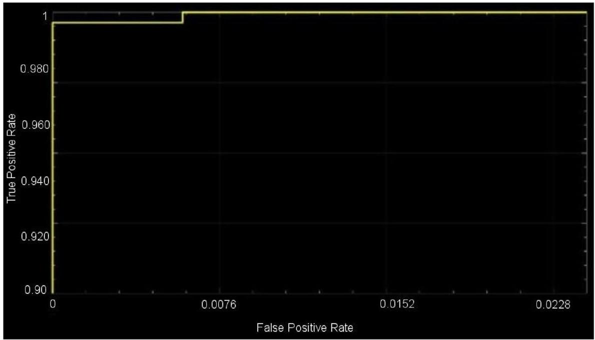
Performance metric evaluation

It is essential to analyze the classification performance in image classification research to provide a rational foundation for the outcomes of the investigation. Many different
performance evaluation metrics have been used for an extended period in studies involving image classification and that have evolved into standard performance evaluation metrics in studies that are similar to the prior. The proposed model used different parametric methods for evaluation, such as precision, sensitivity, and accuracy. These measures, which are generally acknowledged as standard performance evaluation metrics in image classification research, are also employed in this article in order to measure the accuracy and reliability of the classification process. Furthermore, the receiver operation characteristic (ROC) curve area, also known as the AUC of the ROC
Table 1 Number of MRI images in the dataset
Dataset Split-Up
Classification No. of Images in the Group
Mode Group Total No. of Images
1 Malignant 1743 3165
Non-malignant 1422
II Benign 910 4195
Glioma 985
Meningioma 750
Pituitary 750
Metastatic 800
III G-II 1712 4720
G-III 1296
G-IV 1712
curve, is used to evaluate the models’ performance. The following are the equations containing the corresponding formulas for each of these measurements:
where is true positive, is true negative, is false positive, and is false negative.

Experimental Study

We implemented the proposed classification model in MATLAB2021a on a computer with the specifications of 32 GB RAM and an Intel E3-1245v6 @3.70GHz CPU.

Optimization of the Hyperparameters

There have been several developments in the field of medical image processing that have led to the increased use of CNNs, and, as a result, some challenges have arisen in their use. The designs designed to obtain more effective outcomes are deeper, and the input images are becoming higher-quality, which leads to an increase in the amount of processing resources required. Sufficient hardware and tuning the network’s hyperparameters are essential for lowering these computing costs and maximizing results. As a result, the proposed CNN models have nearly all of their essential hyperparameters automatically set using the grid search optimization technique. When the search space for possible values is small, grid search optimization is a great way to improve a CNN’s hyperparameter optimizations. The grid search can select the superior one by training the network through a wide range of possible combinations. CNN models have architectures that are quite complicated and that have a lot of hyperparameters. In most cases, these hyperparameters can
Fig. 2 Proposed CNN model architecture for ” C -1″ mode
Table 2 Detailed information on CNN model employed for “C-1” mode
Layer Name CNN Layer Activations Parameters (Trainable) Total No. of Trainable Parameters
Input nil 0
Convolutional 128 ( ), stride of (4,4), with (0 00 0) padding weights, bias 13,954
Activation layer Activation layer-1 nil 0
Normalization Normalization (cross-channel) nil 0
Max_pooling ( ) with stride of ( 2,2 ), and ( 000 ) padding nil 0
Convolutional 96 ( ), stride of (1,1), and (2 22 2) padding weights, bias 49,246
Activation layer Activation layer-2 nil 0
Max_pooling ( ) with stride of (2,2), and (0 00 0) padding nil 0
Fully_connected 512 Fully_connected weights, bias 11,060,714
Dropout 30% nil 0
Fully_connected 2 Fully_connected weights, bias 1026
Softmax Softmax nil 0
Classification Tumor or non-tumor nil nil 0
Fig. 3 Proposed CNN model architecture for ” C -2″ mode
be arranged into two distinct categories: architectural hyperparameters and fine-adjustment hyperparameters. Architectural hyperparameters include the following: the number of convolutional pooling layers, the number of fully connected layers, the number of filters, the filter
sizes, and the activation function. The regularization, momentum, minibatch size, and learning rate are among the fine-adjustment hyperparameters. In the current analysis, the hyperparameters of the architecture are initially tuned using Algorithm 1.
Table 3 Detailed information on CNN model employed for “C-2” mode
Layer Name CNN Layer Activations Parameters (Trainable) Total No. of Trainable Parameters
Input nil 0
Convolutional , stride of (4,4), with (0 00 0) padding weights, bias 13,952
Activation layer Activation layer-1 nil 0
Normalization Normalization (cross-channel) nil 0
Max_pooling with stride of , and ( 000 ) padding nil 0
Convolutional 96 ( ), stride of (1,1), and (2 22 2) padding weights, bias 442,464
Activation layer Activation layer-2 nil 0
Max_pooling ( ) with stride of ( 2,2 ), and ( 000 ) padding nil 0
Convolutional 96 ( ), stride of ( 1,1 ), and ( 222 2) padding weights, bias 36,960
Activation layer Activation layer-3 nil 0
Max_pooling ( ) with stride of ( 2,2 ), and ( 000 ) padding nil 0
Convolutional 24 ( ), stride of ( 1,1 ), and ( 222 2) padding weights, bias 82,968
Activation layer Activation layer-4 nil 0
Max_pooling ( ) with stride of ( 2,2 ), and ( 000 ) padding nil 0
Convolutional 24 ( ), stride of ( 1,1 ), and ( 222 2) padding weights, bias 20,760
Activation layer Activation layer-5 nil 0
Max_pooling ( ) with stride of ( 2,2 ), and ( 000 ) padding nil 0
Convolutional , stride of (1,1), and (2222) padding weights, bias 12,320
Activation layer Activation layer-6 nil 0
Max_pooling ( ) with stride of ( 2,2 ), and ( 000 ) padding nil 0
Fully_connected 512 Fully_connected weights, bias 16,896
Dropout 30% nil 0
Fully_connected 5 Fully_connected weights, bias 2565
Softmax Softmax nil 0
Classification Benign, glioma, pituitary, metastatic, and meningioma nil nil 0
Algorithm 1. Architectural hyperparameters will be optimized using a grid search algorithm
Begin
Step 1: Assign a 5 -dimensional grid for the 5 hyperparameters needed to be optimized.
Step 2: To each dimension, potential value intervals should be assigned.
– Maximum pooling and convolutional layers = (1,2,3,4)
Step 3: Examine all the potential pairings and choose the one that maximizes overall accuracy.
accuracy
End
After determining the architectural hyperparameters, Algorithm 2 is used to optimize the fine-adjustment hyperparameters. In this proposed study, the grid search is carried out on the training set employing a fivefold crossvalidation method. The dataset is split into five different sets. Four of these sets are used for training, and the fifth set is used for testing. For the Classification-1 mode, there are 3165 images, for the Classification-2 mode, there are 4195 images, and for the Classification- 3 mode, there are 4720 images. For each classification mode, the dataset is randomly split into a training set, a validation set, and a test set, with the ratio being 60:20:20. Basically, the grid search method goes through each possible setting for each parameter and finds the one that gives the best performance. In order to obtain the highest possible degree of accuracy with Algorithm 1, there are five parameters that need to be improved.
Fig. 4 Proposed CNN model architecture for ” C -3″ mode
Algorithm 2. Architectural hyperparameters will be optimized using a grid search algorithm
Begin
Step 1: Assign a 4-dimensional grid for the 5 hyperparameters needed to be optimized.
- Regularization = R2
- A momentum
- Size of the minibatches
- Rate of learning
Step 2: To each dimension, potential value intervals should be assigned.
- R2 = (0.0002, 0.00043, 0.002, 0.004)
- A momentum = (0.78, 0.77, 0.954, and 0.96)
- Size of the minibatches = (4,6, 16, 24, 32, 64)
- Rate of learning = (0.0002, 0.00043, 0.002, 0.004)
Step 3: Examine all the potential pairings and choose the one that maximizes overall ac-
curacy.
- A1 = (0.0002, 16, 0.16, 0.0002) }->mathrm{ accuracy 94.6%
- A2 = (0.0005, 32, 0.9, 0.002) }->mathrm{ accuracy }98.4
- A3 = (0.0002, 64, 0.9, 0.002) }->mathrm{ accuracy }99.2
End
Many possible combinations for these parameters, including , and 4 , correspondingly. As a result, the total number of possible permutations to be examined is , which equals 2240 . Because 2240 combinations need to be checked using the fivefold cross-validation technique, the grid search algorithm created to optimize the CNN model hyper-parameters is carried out 11,200 times. Similar to the first algorithm, the second algorithm has four parameters that need to be optimized to achieve the highest level of accuracy. A wide range of permutations are possible in these parameters,
for example, , and 4 . As a result, the total number of possible permutations that need to be examined is , which equals 320 . Because 320 different possible combinations need possible combinations that need to be tested using the fivefold cross-validation method, the grid search technique developed to improve the correction hyperparameters of the CNN model is carried out a total of 1600 times. As shown in Tables 5, 6 and 7, the grid search optimization algorithm found the best possible values for the hyperparameters of the C-1, C-2, and C-3 modes.

Optimized Convolutional Neural Network Outcomes

The fivefold cross-validation approach for the C-1 mode is utilized to conduct the proposed model’s performance analysis. The dataset is partitioned into five different sets, four of which are utilized for training purposes, while the fifth set is placed to use for testing purposes. There are five total iterations of the experiments, and the classification performance of the mode is evaluated for each fold, and then the overall model’s average classification performance is computed. High accuracy results from the training and validation phases are meaningless if the trained and hyperparametertuned CNN is not tested on its ability to predict samples that have not yet been seen. Hence, to assess the effectiveness of the trained CNN to assess the trained
Table 4 Detailed information on CNN model employed for “C-3” mode
Layer Name CNN Layer Activations Parameters (Trainable) Total No. of Trainable Parameters
Input nil 0
Convolutional 128 ( ), stride of (4,4), with (0 00 0) padding weights, bias 13,952
Activation layer Activation layer-1 nil 0
Normalization Normalization (cross-channel) nil 0
Max_pooling ( ) with stride of ( 2,2 ), and ( 000 ) padding nil 0
Convolutional 96 ( ), stride of (1,1), and (2 22 2) padding weights, bias 46,752
Activation layer Activation layer-2 nil 0
Max_pooling ( ) with stride of ( 2,2 ), and ( 000 ) padding nil 0
Convolutional 96 ( ), stride of ( 1,1 ), and ( 222 2) padding weights, bias 36,864
Activation layer Activation layer-3 nil 0
Max_pooling ( ) with stride of (2,2), and (0 00 0) padding nil 0
Fully_connected 512 Fully_connected weights, bias 3,146,240
Dropout 30% nil 0
Fully_connected 3 Fully_connected weights, bias 1539
Softmax Softmax nil 0
Classification G-II, G-III, G-IV nil nil 0
CNN’s effectiveness on predicting samples, a test dataset is randomly allocated and segregated alongside the training and validation datasets. If this step is skipped, the high accuracy may result from biased dataset assignment. Table 8 displays the results of randomly splitting the 3165 images from the study into the training, validation, and test sets in the ratio of 60:20:20 for the C-1 mode.
A total of 299 images are taken randomly from the dataset for each category, and then those images are used for testing. The activations of the CNN’s convolution layers can be displayed for a better view of the features
Table 5 The grid search-yielded optimal results for the hyperparameters for the C-1 mode
Hyperparameters Changes in Parameter Values Maximal Value
Layers of maximum pooling and CNN (1, 2, 3, 4) 2
Number of layers that are completely connected (1, 2, 3, 4) 2
Total number of filters (8, 16, 24, 32, 48, 64, 96, 128, 256) 64,96,128
Intensity of filtration (3, 4, 5, 6, 7) 6,6
Role of activation (ReLU, ELU, Leaky ReLU) ReLU
Size of minibatch (4, 6, 16, 24, 32, 64) 32
Rate of change (0.78, 0.77, 0.95, 0.96) 0.95
Rate of learning (0.0002, 0.00043, 0.002, 0.004) 0.0002
-regularization (0.0002, 0.00043, 0.002, 0.004) 0.0002
that the CNN has learned due to its training. With this representation, the researcher may easily observe the network’s progress. Figures 5 and 6 each depict the activations of the first and second convolutional layers. One of the images in the grid serves as a representation of the channel’s outcome. White areas represent highly positive activations, while grey areas represent moderately activated channels. While the first convolutional layer of the CNN is used to learn features such as color and edges, the second convolutional layer is used to learn more complex information, such as the borders of brain tumors. The succeeding (deeper) convolutional layers
Table 7 The grid search-yielded optimal results for the hyperparameters for the C-3 mode
Hyperparameters Changes in Parameter Values Maximal Value
Layers of maximum pooling and CNN (1, 2, 3, 4) 3
Number of layers that are completely connected (1, 2, 3, 4) 2
Total number of filters (8, 16, 24, 32, 48, 64, 96, 128, 256) 64, 96, 128
Intensity of filtration (3, 4, 5, 6, 7) 6, 6, 4
Role of activation (ReLU, ELU, Leaky ReLU) ReLU
Size of minibatch (4, 6, 16, 24, 32, 64) 32
Rate of change (0.78, 0.77, 0.95, 0.96) 0.95
Rate of learning (0.0002, 0.00043, 0.002, 0.004) 0.004
-regularization (0.0002, 0.00043, 0.002, 0.004) 0.002
Table 6 The grid search-yielded optimal results for the hyperparameters for the C-2 mode
Hyperparameters Changes in Parameter Values Maximal Value
Layers of maximum pooling and CNN (1, 2, 3, 4) 6
Number of layers that are completely connected (1, 2, 3, 4) 2
Total number of filters (8, 16, 24, 32, 48, 64, 96, 128, 256) 16, 24, 32, 48, 64, 96, 128
Intensity of filtration (3, 4, 5, 6, 7) 6, 6, 4, 6, 2, 6
Role of activation (ReLU, ELU, Leaky ReLU) ReLU
Size of minibatch (4, 6, 16, 24, 32, 64) 64
Rate of change (0.78, 0.77, 0.95, 0.96) 0.95
Rate of learning (0.0002, 0.00043, 0.002, 0.004) 0.0002
-regularization (0.0002, 0.00043, 0.002, 0.004) 0.002
build up their features by merging the features learned by the earlier convolutional layers.
Figure 5 shows 96 of the 128 channels in the CNN’s first convolutional layer running in C-1 mode. This layer contains a total of 128 channels. Figure 6 shows an image of the second convolutional layer of the network, which has 96 channels. Every layer of the CNN is composed of channels, which are arrays in two dimensions. One of the images in Fig. 5 represents the output of each channel in the first convolutional layer. In these images, strong positive activations are shown by white pixels, and strong negative activations are shown by black pixels. Similarly, grey pixels on the input image indicate channels that are not highly active. Figure 7 depicts the activations of a particular channel and the channel with the most significant activation in the first convolutional layer. The presence of white pixels in the channel of Fig. 7 demonstrates that this channel is highly activated at the tumor’s location. Although the CNN was never instructed to learn about tumors, it is possible to conclude that it has picked up on the fact that tumors have distinguishing qualities that allow it to differentiate between different categories of images.
These CNNs are able to discover helpful characteristics on their own, unlike earlier artificial neural network methods that typically required manual design to fit a particular mode. In this proposed article, learning to recognize tumors improves the ability to distinguish between a tumor image and non-tumor image. After the process of classification has been completed, the efficiency of the CNN models must be evaluated using different reliable approaches. The metrics, like the specificity, sensitivity, precision, and accuracy measures, as well as the area under the ROC curve, are used to perform the performance evaluation of the proposed model. The proposed CNN’s loss and accuracy plots for the C-1 mode are shown in Fig. 8. After 340 iterations, the model proposed for C-1 was able to classify with a accuracy. It is pretty clear, as shown in Fig. 8, that approximately 250 iterations are required to reach an almost perfect level of accuracy. Figure 9 depicts the confusion matrix for the Classification-1 mode. As can be seen in Fig. 10, the area under the ROC curve has a value of 0.9995 for its AUC. The results presented here demonstrate that the recommended CNN model is capable of identifying brain tumors. Table 9 shows the measures of
Table 8 Training, validating, and testing phases of proposed CNN model
Dataset Split-Up Training, Validation, and Testing Modes
Classification No. of Images in the Group Total No. of Images Training Mode (60%) Validation Mode (20%) Test Mode (20%)
1 Malignant 1743 3165 1899 633 633
Non-malignant 1422
II Benign 910 4195 2517 839 839
Glioma 985
Meningioma 750
Pituitary 750
Metastatic 800
III G-II 1712 4720 2832 944 944
G-III 1296
G-IV 1712
Fig. 5 First CNN activation layer for C-1 mode
Fig. 6 Second CNN activation layer for C-1 mode
the accuracy, such as the true positive (TP), true negative (TN), false positive (FP), false negative (FN), accuracy (Acc), specificity (Sp), sensitivity (Se), and precision (Pr). Figure 10 depicts the ROC curve for the Classification-1 (C-1) task.
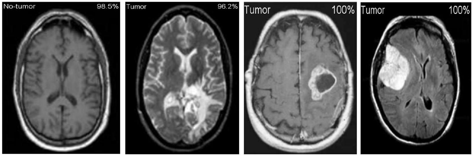
Figure 11 shows the results of the classification and the predicted probabilities for each of the four tests conducted in C-1 mode. Implementing the fivefold cross-validation method for the mode evaluates the effectiveness of the proposed framework. The dataset is partitioned into five sets, four of which are utilized
for training purposes, while the fifth set is placed for testing purposes. There are five total iterations of the experiments. The classification performance of the job is evaluated for each fold, and then the overall model’s average classification performance is computed. As indicated in Table 8, there are sufficient images for the -mode training, validation, and test sets to be randomly divided in a ratio of for a sample size of 4195 . From the dataset of each class that will be used to test the model, 158 images are randomly selected to be removed. The accuracy and loss plots of the suggested CNN model for
Fig. 7 C-1-mode strongest and moderate images from original input image
Fig. 8 C-1-mode accuracy and loss curves
the C-2 task are displayed in Fig. 12. The proposed CNN method for the C-2 mode achieves a 93.81% accuracy in classification after 294 iterations. As shown in Fig. 13, the area under the ROC curve has a value of 0.9981 . These findings demonstrate the proposed CNN model’s capability to classify brain tumor types. Figure 14 depicts a confusion matrix, and Table 9 lists the many measures of precision, such as TP, TN, FP, FN, Acc, Sp, Se, and Pr. According to Table 9, an accuracy of is attained when classifying a glioma, when classifying a meningioma, when classifying metastasis, when classifying a healthy brain, and when classifying the pituitary tumor type for the C-2 mode.
Figure 14 depicts the ROC curve for the Classification-2 (C-2) task.
The fivefold cross-validation process for the C-3 mode is utilized to evaluate the efficacy of the proposed models. The dataset is partitioned into five different sets, out of which four are used for training and the fifth is used for testing. There are five total iterations of the experiments. Following an analysis of the classification performance of the mode for each fold, an average classification performance for the model is computed. For the C-3 mode, sufficient images can be randomly divided into training, validation, and test sets in the proportions 60:20:20, as indicated in Table 8, randomly excluding three hundred
Target Class
Non tumor 268 44.9% 3 0.6% 98.72% 1.28%
Output Class Tumor 0 0.0% 326 54.1% 100% 0.0%
100% 0.0% 98.9% 1.1% 99.5% 0.6%
Tumor Non tumor Total
Fig. 9 C-1 confusion matrix
Fig. 10 C-1-mode average of ROC curve
and five images from the dataset of each class to be utilized to evaluate the model. The loss and accuracy graphs of the proposed CNN for the C-3 mode are shown in Fig. 15. Figure 16 depicts the confusion matrix for the C-3 mode. The proposed approach for the C-3 mode obtains a classification accuracy of after 344 iterations. Figure 17 depicts the ROC curve for the Classi-fication-3 (C-3) task. Table 9 shows that an accuracy of is reached when classifying grade II, when
classifying grade III, and when classifying grade IV for brain tumor grades in the C-3 mode. The three different classification outcomes of the proposed CNN model were compared with other conventional CNN approach outcomes to evaluate the proposed system classification ability. To achieve this goal, the same experiments were performed with the same dataset, utilizing well-known and popular pretrained CNN models, such as AlexNet, DenseNet121, ResNet-101, VGG-16, and
Table 9 Proposed CNN model parameter metric outcomes for all classification modes
Metrics Classes TP TN FP FN Acc Sp Se Pr Total
1 Malignant 268 326 3 0 99.50 99.09 100.00 98.89 268
Non-malignant 326 268 0 3 99.50 100.00 99.09 100.00 329
II Benign 183 598 8 8 97.99 98.68 95.81 95.81 191
Glioma 132 650 10 12 97.26 98.48 91.67 92.96 144
Meningioma 138 643 6 14 97.50 99.08 90.79 95.83 152
Pituitary 160 598 24 11 95.59 96.14 93.57 86.96 171
Metastatic 127 643 11 14 96.86 98.32 90.07 92.03 141
III G-II 332 574 9 8 98.16 98.46 97.65 97.36 340
G-III 248 679 0 0 100.00 100.00 100.00 100.00 248
G-IV 330 580 8 9 98.17 98.64 97.35 97.63 339
Fig. 11 The results of classification and predictions for the probabilities of four different test images for the C-1 mode
Fig. 12 C-2-mode accuracy and loss curves
Fig. 13 C-2-mode average of ROC curve
Target Class
Glioma 183 3 4 1 0 95.9%
22.8% 0.4% 0.5% 0.1% 0.0% 4.1%
Meningioma 4 132 3 1 2 93.8%
0.5% 16.3% 0.4% 0.1% 0.3% 6.2%
Output Class Metastatic 1 2 138 2 1 95.9%
0.1% 0.3% 17.4% 0.3% 0.1% 4.1%
Benign 3 4 6 160 11 86.8%
0.4% 0.5% 0.8% 20.2% 1.4% 13.2%
Pituitary 0 3 1 7 127 93.1%
0.0% 0.4% 0.1% 0.9% 15.9% 6.9%
95.3% 93.9% 92.7% 93.6% 90.0% 93.8%
4.7% 6.1% 7.3% 6.4% 10.0% 6.9%
Glioma Meningioma Metastatic Benign Pituitary Total
Fig. 14 C-2 confusion matrix
GoogleNet. Table 10 illustrates the performance metric outcome comparison of the proposed CNN model with existing CNN approaches. Figure 18 depicts the graphical representation of the proposed and existing models’ result comparison.
The results shown in Table 10 illustrate that the proposed CNN models outperform other networks in every classification mode. The pretrained DenseNet121
model, which obtains a classification accuracy in the brain tumor detection test ( mode), is the model that is closest to the suggested model. The pretrained VGG-16 model obtains an accuracy in the brain tumor-type classification mode (C-2 mode). It is the model that is closest to the proposed CNN model. After the proposed CNN model, the pretrained GoogleNet model achieves a classification accuracy of
Fig. 15 C-3-mode accuracy and loss curves
Target Class
GII 332 37.2% 0 0.0% 9 1.1% 97.7% 2.3%
Output Class
0 0.0% 248 26.1% 0 0.0% 100% 0.0%
8 0.8% 0 0.0% 330 35.1% 98.1% 1.9%
100% 0.0% 97.5% 2.5% 98.1% 1.9% 98.5% 1.5%
GII GIII GIV Total
Fig. 16 C-3 confusion matrix
95.12%, making it the best network available for grading tumors (C-3 mode). It is clear that the proposed CNN models are better than the pretrained networks, which were built and trained using generic datasets and methods for a wide range of image classification tasks. Table 11 illustrates the proposed and existing model outcome comparison. The proposed CNN models, conversely, were designed to deal with more specific issues, like identifying and defining various types and stages of brain tumors. Finally, MRI images of brain tumors are used to train and evaluate the proposed models.

Conclusions

In this research, we propose a multi-classification method for identifying brain tumors at an early stage using (CNN) models, in which nearly all the hyperparameters are automatically optimized via grid search. By using publicly available medical imaging datasets, three reliable CNN models have been designated to perform three distinct brain tumor classification tasks. A high level of accuracy, such as , can be attained in the process of detecting brain tumors. In addition, a remarkable accuracy of is achieved
Fig. 17 C-3-mode average of ROC curve
Table 10 Performance metric outcome comparison of the proposed CNN model with existing CNN approaches
CNN Models C-1 Mode C-2 Mode C-3 Mode
Acc (%) AUC Acc (%) AUC Acc (%) AUC
GoogleNet 74.21 0.8108 77.89 0.8212 95.12 0.9617
AlexNet 89.23 0.8989 84.24 0.8501 91.08 0.9772
DenseNet121 93.89 0.9412 77.67 0.8122 86.07 0.8809
ResNet101 93.29 0.9442 76.45 0.8115 86.42 0.881
VGG-16 88.87 0.9201 89.19 0.8112 84.87 0.8663
Proposed CNN approach 99.53 0.9994 93.81 0.9984 98.56 0.9993
Fig. 18 Graphical illustration of proposed and existing models’ outcome comparison
Table 11 Comparison of the proposed model with existing studies
Author Year Datasets Method Classification of Accuracy (%)
Ahmed Wasif Reza [12] 2023 Kaggle, Figshare VGG-16 architecture 96.70
Mahmoud Khaled Abd-Ellah [13] 2018 RIDER, REMBRANDT, and BraTS ECOC-SVM 97.98
Takowa Rahman [27] 2023 Kaggle, REMBRANDT CNN + 6 pretrained models 97.12
Anand Deshpande [17] 2021 RIDER and BraTS Discrete cosine transform-based image fusion combined with CNN 98.14
Proposed model 2023 Figshare, REMBRANDT, TCGA-LGG, TCIA Hybrid CNN 98.56
when classifying brain MR images into the categories of glioma, meningioma, pituitary, normal brain, and metastatic. The final step is grading glioma brain tumors, which can be performed with an accuracy of for grades II, III, and IV. A good number of medical images are used to train and test the CNN models that are being proposed. Results from the proposed CNN models and comparisons with current methods show that CNN models made with the proposed optimization framework work well. In this work, CNN models were made that can help clinicians and radiologists check primary screenings for multiple types of brain tumors.

Acknowledgements

Not applicable.

Institutional Review Board Statement

Not applicable.

Human Participants Research Checklist:

Complete the following if your study involved human participants or human participants’ data. These questions should be addressed for prospective and retrospective studies.
  1. Did you obtain ethics approval for this study?
  • If yes, please upload (file type “Other”) the original approval document you received from your ethics committee. If the original document is in another language, please also provide an English translation.
    Response: N/A
  • If you did not obtain ethical approval, please explain why this was not required below.
  1. If you prospectively recruited human participants for the study for example, you conducted a clinical trial, distributed questionnaires, or obtained tissues, data or samples for the purposes of this study, please report in the Methods: i. the day, month and year of the start and end of the recruitment period for this study.
    ii. whether participants provided informed consent, and if so, what type was obtained (for instance, written or verbal, and if verbal, how it was documented and witnessed). If your study included minors, state whether you obtained consent from parents or guardians. If the need for consent was waived by the ethics committee, please include this information.
    Response: N/A
  2. If you are reporting a retrospective study of medical records or archived samples, please report in the Methods section:
    i. the day, month and year when the data were accessed for research purposes ii. whether authors had access to information that could identify individual participants during or after data collection
    Response: N/A

Authors’ contributions

Conceptualization, S.S. and D.F.; methodology, S.K.M. and H.R.; valida-tion, H.R. and M.A.S.; data curation, B.D.S.; writing —original draft, S.S. and D.F.; writing — review and editing, S.K.M. and H.R.; visualization, B.D.S; supervision S.K.M., and M.A.S.; project ad-ministration, S.K.M., and M.A.S. All authors have read and agreed to the published version of the manuscript.

Funding

This research received no external funding.

Availability of data and materials

The datasets used during the current study are available from the corresponding author upon reasonable request.

Declarations

Not applicable.

Competing of interests

The authors declare no competing interests.
Received: 7 November 2023 Accepted: 8 January 2024
Published online: 19 January 2024

References

  1. Abiwinanda N, Hanif M, Hesaputra ST, Handayani A, Mengko TR. Brain tumor classification using convolutional neural network. IFMBE Proc. 2019;68:183-9.
  2. Ayadi W, Elhamzi W, Charfi I, Atri M. Deep CNN for brain tumor classification. Neural Process Lett. 2021;53:671-700.
  3. Badža MM, Barjaktarović MČ. Classification of brain tumors from MRI images using a convolutional neural network. Appl Sci. 1999;2020:10.
  4. Saravanan S, Kumar VV, Sarveshwaran V, Indirajithu A, Elangovan D, Allayear SM. Computational and Mathematical Methods in Medicine Glioma Brain Tumor Detection and Classification Using Convolutional Neural Network. Comput Math Methods Med. 2022;2022:4380901.
  5. Ge C, Gu IYH, Jakola AS, Yang J. Deep semi-supervised learning for brain tumor classification. BMC Med Imaging. 2020;20:87.
  6. Cinar A, Yildirim M. Detection of tumors on brain MRI images using the hybrid convolutional neural network architecture. Med Hypotheses. 2020;139: 109684.
  7. Pei L, Vidyaratne L, Rahman MM, Iftekharuddin KM. Context aware deep learning for brain tumor segmentation, subtype classification, and survival prediction using radiology images. Sci Rep. 2020;10:19726.
  8. Balasooriya NM, Nawarathna R.D. A sophisticated convolutional neural network model for brain tumor classification. In Proceedings of the 2017 IEEE International Conference on Industrial and Information Systems, Peradeniya, Sri Lanka, 15-16 2017; pp. 1-5
  9. Deepak VK, Sarath R. Multi-Class Brain Cancer Classification Using Deep Learning Convolutional Neural Network. PalArch’s J Archaeol Egypt/Egyptol. 2020;17:5341-60.
  10. Khan HA, Jue W, Mushtaq M, Mushtaq MU. Brain tumor classification in MRI image using convolutional neural network. Math Biosci Eng. 2020;17:6203-16.
  11. Islam R, Imran S, Ashikuzzaman M, Khan MMA. Detection and Classification of Brain Tumor Based on Multilevel Segmentation with Convolutional Neural Network. Biomed Sci Eng. 2020;13:45-53.
  12. Reza AW, Hossain MS, Wardiful MA, Farzana M, Ahmad S, Alam F, Nandi RN, Siddique N. A CNN-Based Strategy to Classify MRI-Based Brain Tumors Using Deep Convolutional Network. Appl Sci. 2023;13:312.
  13. Abd-Ellah MK, Awad AI, Khalaf AA, Hamed HF. Two-phase multi-model automatic brain tumor diagnosis system from magnetic resonance images using convolutional neural networks. EURASIP J Image Video Process. 2018;97:1-10.
  14. Noreen N, Palaniappan S, Qayyum A, Ahmad I, Alassafi MO. Brain Tumor Classification Based on Fine-Tuned Models and the Ensemble Method. Comput Mater Contin. 2023;67:3967-82. https://doi.org/10.32604/cmc. 2021.014158.
  15. Mohsen H, El-Dahshan ESA, El-Horbaty ESM, Salem ABM. Classification using deep learning neural networks for brain tumors. Future Comput Inform J. 2018;3:68-71.
  16. Chattopadhyay A, Maitra M. MRI-based brain tumor image detection using CNN based deep learning method. Neurosci Inform. 2022;2:100060.
  17. Deshpande A, Estrela VV, Patavardhan P. The DCT-CNN-ResNet50 architecture to classify brain tumors with super-resolution, convolutional neural network, and the ResNet50. Neurosci Inform. 2021;1:100013.
  18. Wankhede DS, Selvaran R. Dynamic architecture based deep learning approach for glioblastoma brain tumor survival prediction. Neurosci Inform. 2022;2:100062.
  19. Rai HM, Chatterjee K. Detection of brain abnormality by a novel Lu-Net deep neural CNN model from MR images. Mach Learn Appl. 2020;2:100004.
  20. Ramya M, Kirupa G, Rama A. Brain tumor classification of magnetic resonance images using a novel CNN-based medical image analysis and detection network in comparison with AlexNet. J Popul Ther Clin Pharmacol. 2022;29:e97-108. https://doi.org/10.47750/jptcp.2022.898.
  21. Bingol H, Alatas B. Classification of Brain Tumor Images using Deep Learning Methods. Turk J Sci Technol. 2021;16:137-43.
  22. Acquarelli J, van Laarhoven T, Postma GJ, Jansen JJ, Rijpma A, van Asten S, Heerschap A, Buydens LMC, Marchiori E. Convolutional neural networks to predict brain tumor grades and Alzheimer’s disease with MR spectroscopic imaging data. PLoS ONE. 2021;7:e0268881.
  23. Bhandari A, Koppen J, Agzarian M. Convolutional neural networks for brain tumor segmentation. Insights Imaging. 2020;11:1-9.
  24. Shelatkar T, Urvashi D, Shorfuzzaman M, Alsufyani A, Lakshmanna K. Diagnosis of Brain Tumor Using Light Weight Deep Learning Model with Fine-Tuning Approach. Comput Math Methods Med. 2022;2022:285884.
  25. Shwetha V, Madhavi CR, Nagendra KM. Classification of Brain Tumors Using Hybridized Convolutional Neural Network in Brain MRI images. Int J Circuits Syst Signal Process. 2022;16:561-70.
  26. Anagun Y. Smart brain tumor diagnosis system utilizing deep convolutional neural networks. Multimed Tools Appl. 2023;675:1-27.
  27. Rahman T, Islam MS. MRI brain tumor detection and classification using parallel deep convolutional neural networks. Meas Sens. 2023;26:100694.
  28. AI-Zoghby AM, AI-Awadly EMK, Moawad A, Yehia N, Ebada AI. Dual Deep CNN for Tumor Brain Classification. Diagnostics. 2023;13:2050.
  29. Saeedi S, Rezayi S, Keshavarz HR, Niakan Kalhori S. MRI-based brain tumor detection using convolutional deep learning methods and chosen machine learning techniques. BMC Med Inform Decis Mak. 2023;23:1-17.
  30. Srinivasan S, Bai PSM, Mathivanan SK, Muthukumaran V, Babu JC, Vilcekova L. Grade Classification of Tumors from Brain Magnetic Resonance Images Using a Deep Learning Technique. Diagnostics. 2023;13:1153.
  31. Yin Z, Gao H, Gong J, Wang Y. WD-UNeXt: Weight loss function and dropout U-Net with ConvNeXt for automatic segmentation of few shot brain gliomas. IET Image Process. 2023;17:3271-80.
  32. Prasad V, Vairamuthu S, Selva Rani B. K-Net-Deep joint segmentation with Taylor driving training optimization based deep learning for brain tumor classification using MRI. The Imaging Sci J. 2023. https://doi.org/10.1080/ 13682199.2023.2208963.
  33. Barboriak D. Data from RIDER_NEURO_MRI. Cancer Imag Arch. 2015. https://doi.org/10.7937/K9/TCIA.2015.VOSN3HN1.
  34. Lisa S, Flanders Adam E, Mikkelsen JR, Tom Andrews DW. Data From REMBRANDT. Arch: Cancer Imag; 2015. https://doi.org/10.7937/K9/TCIA. 2015.588OZUZB.
  35. Pedano N, Flanders AE, Scarpace L, Mikkelsen T, Eschbacher JM, Hermes B, Ostrom Q. Radiology data from the cancer genome atlas low grade glioma [TCGA-LGG] collection. Cancer Imag Arch. 2016. https://doi.org/ 10.7937/K9/TCIA.2016.L4LTD3TK.
  36. Clark K, Vendt B, Smith K, Freymann J, Kirb J, Koppel P, Moore S, Phillips S, Maffitt D, Pringle M. The cancer imaging archive (TCIA): Maintaining and operating a public information repository. J Digit Imaging. 2013;26:1045-57.
  37. Cheng J, Huang W, Cao S, Yang R, Yang W, Yun Z, Wang Z, Feng Q. Enhanced performance of brain tumor classification via tumor region augmentation and partition. PLoS ONE. 2015;10: e0140381.
  38. Rahim T, Usman MA, Shin SY. A survey on contemporary computer-aided tumor, polyp, and ulcer detection methods in wireless capsule endoscopy imaging. Comput Med Imaging Graph. 2020;85: 101767.
  39. Rahim T, Hassan SA, Shin SY. A deep convolutional neural network for the detection of polyps in colonoscopy images. Biomed Signal Process Control. 2021;68: 102654.

Publisher’s Note

Springer Nature remains neutral with regard to jurisdictional claims in published maps and institutional affiliations.

  1. *Correspondence:
    Mohd Asif Shah
    drmohdasifshah@kdu.edu.et
    ¹ Department of Computer Science and Engineering, Vel Tech Rangarajan Dr.Sagunthala R&D Institute of Science and Technology, Chennai 600062, India
    Department of Electronics and Communication Engineering, PSNA College of Engineering and Technology, Dindigul 624622, India
    School of Computing Science and Engineering, Galgotias University, Greater Noida 203201, India
    School of Computing Science and Engineering, VIT Bhopal University, Bhopal-Indore Highway Kothrikalan, Sehore 466114, India
    Department of Economics, Kabridahar University, Po Box 250, Kebri Dehar, Ethiopia
    Centre of Research Impact and Outcome, Chitkara University Institute of Engineering and Technology, Chitkara University, Rajpura, Punjab, 140401, India
    Division of Research and Development, Lovely Professional University, Phagwara, Punjab, 144001, India