نهج التجميع الطيفي لمعادلة كورتويغ-دي فريس-بورجرز ذات الكسر الزمني عبر متعددات حدود تشيبيشيف من النوع الأول A Spectral Collocation Approach for Time-Fractional Korteweg-de Vries-Burgers Equation via First-Kind Chebyshev Polynomials

المجلة: Contemporary Mathematics
DOI: https://doi.org/10.37256/cm.6220255948
تاريخ النشر: 2025-02-28

نهج التجميع الطيفي لمعادلة كورتويغ-دي فريس-بورجرز ذات الكسر الزمني عبر متعددات حدود تشيبيشيف من النوع الأول

ي. ح. يسري , ليلى أ. الناصر , أ. ج. عطاء 1قسم الرياضيات، كلية العلوم، جامعة القاهرة، الجيزة، 12613، مصر كلية الهندسة، جامعة مصر للمعلوماتية، مدينة المعرفة، العاصمة الإدارية الجديدة، 19519، مصر قسم الرياضيات، كلية العلوم، جامعة طيبة، المدينة المنورة، 41411، المملكة العربية السعودية قسم الرياضيات، كلية التربية، جامعة عين شمس، روكسي، 11341، القاهرة، مصرالبريد الإلكتروني: lnaser@taibahu.edu.sa

تاريخ الاستلام: 21 أكتوبر 2024؛ تاريخ المراجعة: 6 فبراير 2025؛ تاريخ القبول: 10 فبراير 2025

الملخص

تم حل مشكلة كورتويغ-دي فريس-برجرز ذات الكسر الزمني (TFKdVB) عددياً في هذه الدراسة. يستخدم النهج طريقة التراص لمتعددات شبيشيف من النوع الأول المنقولة (SFKCPs). من خلال استخدام صيغة كابوتو لتقريب المشتقات ذات الكسر الزمني وفرض شروط الحدود، نصل إلى حل طيفي. تم تقديم أمثلة عددية لتوضيح دقة وفعالية النهج المقترح.

الكلمات المفتاحية: متعددات شبيشيف من النوع الأول، طريقة التراص، معادلة كورتويغ-دي فريس-برجرز ذات الكسر الزمني
MSC: 35R11، 65M70، 35Q53، 41A10، 65N35

1. المقدمة

طور كورتويغ ودي فريس [1] معادلة كورتويغ-دي فريس (KdV) في عام 1895 لتحسين فهم ديناميات الموجات غير الخطية الضعيفة. منذ نشأتها، كانت هذه المعادلة أداة أساسية لدراسة مجموعة واسعة من الظواهر الفيزيائية في مجالات مختلفة. طور سو وغاردنر [2] معادلة (KdVB)، التي تعتبر مفيدة بشكل خاص للتحقيق في تفاعل التشتت، والتبدد، وغير الخطية في انتشار الموجات عبر قناة مرنة مملوءة بالسوائل. علاوة على ذلك، فإن معادلة TFKdVB ذات الكسر [3]، ومعادلة شرودنجر-كورتويغ-دي فريس ذات الكسر [4]، ومعادلة برجرز ذات الكسر [5] هي معادلات تفاضلية جزئية غير خطية حديثة مقترحة لشرح الظواهر الحرجة والعمليات الديناميكية المعقدة في مجال الفيزياء. تعتبر معادلة KdVB أداة أساسية تستخدم لوصف العديد من العمليات العلمية، بما في ذلك انتشار الموجات، ونماذج تدفق المرور، وديناميات السوائل. إن امتداد الشكل الكلاسيكي، الذي يتضمن مشتقاً كسرية بالنسبة للزمن [6-8]، هو معادلة TFKdVB، مما يتيح تمثيل الانتشار الشاذ والسلوك غير المحلي. توفر المشتقات الكسرية تصويراً أكثر دقة لبعض الأنظمة الفيزيائية لأنها تعكس ميزات الذاكرة والوراثة للعمليات ذات الصلة. بسبب ذلك، تعتبر معادلة TFKdVB أداة أساسية لفهم الديناميات المعقدة التي لا يمكن التعبير عنها في نماذج الأعداد الصحيحة القياسية [9-11].
هناك العديد من التطبيقات الواقعية لمعادلة TFKdVB. يمكن أن تحاكي تدفق السوائل في الأنابيب، على سبيل المثال، حيث تؤثر تأثيرات الذاكرة على التدفق. إنها مفيدة بشكل خاص في تفسير كيفية تصرف الموجات في مواد مثل المواد الصلبة المرنة، حيث تكون خصائص المواد والتأثيرات الزمنية مهمة.
تعتبر هذه المعادلة مفيدة في الأبحاث البيئية لأنها يمكن أن تستخدم أيضاً للتنبؤ بتشتت الملوثات في الأنهار أو المحيطات، حيث يتأثر التشتت بالظروف التاريخية. تقنياً، جذبت المعادلات ذات الكسر الزمني انتباه العديد من الباحثين بسبب نطاق تطبيقاتها الواسع. تم تطوير عدة طرق لمعالجة المعادلات ذات الكسر الزمني، بما في ذلك طريقة الشريحة غير متعددة الحدود الكسرية، وطريقة الاضطراب الهوموتوبية، وطريقة الشريحة غير متعددة الحدود الهايبر بولية، وطريقة الأنزاتز [12-14].
أثبتت متعددات شبيشيف، وهي عائلة من متعددات orthogonal، فعاليتها العالية في التحليل العددي، خاصة في حل المعادلات التفاضلية. تجعل خصائص التقريب القوية لها مناسبة جداً للطرق الطيفية. عندما تكون الدقة العالية مطلوبة، تبسط علاقاتها التكرارية وorthogonality المشاكل المعقدة. تسهل متعددات شبيشيف وصف الحلول في شكل سلسلة عند حل المعادلات التفاضلية الكسرية، مما يوفر طريقة فعالة لتقريب الحلول على مدى فترة محددة [15-18].
تعتبر طريقة التراص الطيفي تقنية عددية دقيقة للغاية لحل المعادلات التفاضلية، خاصة تلك التي تتضمن مشتقات كسرية. تعمل عن طريق تقسيم المجال إلى نقاط تراص، حيث يجب أن تلبي الحلول المعادلة بدقة، مما يحول المعادلة التفاضلية إلى نظام من المعادلات الجبرية. تعمل هذه الاستراتيجية بشكل جيد بشكل خاص لأنها تجمع بين سهولة استخدام تقنيات التراص وسرعة التقارب للطرق الطيفية. تصبح طريقة التراص الطيفي أداة فعالة لحل المعادلات التفاضلية الكسرية التي تكون خطية وغير خطية عند دمجها مع متعددات شبيشيف [19، 20].
تمت دراسة تطبيق الطرق الطيفية لحل المعادلات التفاضلية الكسرية في عدد من المنشورات. بسبب دقتها وفعاليتها، تم استخدام طرق طيفية مثل بترون-غاليركين، وغاليركين، وطرق التراص في النماذج الكسرية في السنوات الأخيرة. أظهرت الأبحاث أن الطرق الطيفية، خاصة عند دمجها مع متعددات orthogonal مثل شبيشيف أو ليجندر، يمكن أن تحقق نتائج عالية الدقة حتى مع عدد أقل من نقاط التراص. علاوة على ذلك، قام العديد من الباحثين بتطبيق هذه الطرق على المعادلات ذات الكسر الزمني، مما يظهر إمكانياتها في نمذجة الأنظمة الفيزيائية ذات الخصائص الذاكرية والوراثية [21-27].
سلطت الأعمال الأخيرة في الطرق العددية لمشاكل الكسر الضوء على الحاجة إلى طرق قوية وفعالة للتعامل مع الصعوبات التي تقدمها هذه المعادلات. بسبب عدم خطيتها ووجود مشتقات كسرية، تعتبر معادلة TFKdVB صعبة بشكل خاص. استجابة لذلك، استكشف العلماء عددًا من التقنيات العددية، بما في ذلك الطرق الطيفية، والفرق المحدود، وطرق العناصر المحدودة، لتقديم تقريبات دقيقة للغاية للحلول. تشتهر الطرق الطيفية بخصائص التقارب الاستثنائية وفعاليتها الحسابية، خاصة عند اقترانها مع متعددات orthogonal مثل شبيشيف أو ليجندر. من خلال تقديم مجموعة من SFKCPs المصممة لحل مشكلة TFKdVB بدقة وفعالية، توسع هذه الدراسة على التطورات السابقة. في هذه الدراسة، نقدم طريقة لحل معادلة TFKdVB تعتمد على متعددات شبيشيف للتراص الطيفي. ثم يتم تقسيم المجال المكاني باستخدام طريقة التراص الطيفي، ويتم حل النظام الناتج من المعادلات. يتم استخدام العديد من الأمثلة العددية التي تظهر تقارب الطريقة المقترحة للتحقق من دقة النهج. تظهر نتائجنا أنه، حتى مع عدد محدود نسبياً من نقاط التراص، توفر طريقة التراص الطيفي حلاً موثوقًا وفعالًا لمعادلة TFKdVB.
يقدم النهج المقترح استخدامًا جديدًا لمجموعات SFKCPs المعدلة في طريقة التراص، مما يوفر مخططًا عدديًا دقيقًا وفعالًا وسريعًا لحل معادلة TFKdVB طيفيًا. يتناول صعوبات مهمة في التعقيد الحسابي والاستقرار، مستخدمًا موارد حاسوبية قليلة ويحسن بشكل كبير دقة الحل مقارنة بالنهج الحالية. إلى أفضل ما لدينا من المعرفة، يمكن سرد المساهمة الرئيسية والجدة في هذه الورقة في النقاط التالية:
  • تم تقديم خلفية نظرية جديدة لمجموعات SFKCPs.
  • اشتقاق نظريات جديدة للمشتقات الصحيحة والكسرية لمجموعات SFKCPs المعدلة. تعتبر هذه النظريات أدوات مهمة لمعالجة TFKdVB.
مزايا النهج المقدم هي كما يلي.
  • من خلال اختيار مجموعات SFKCPs المعدلة كدوال أساسية، تجعل بعض مصطلحات الأوضاع المحتفظ بها تنتج تقريبًا بدقة واعدة.
  • تتطلب الحصول على الحل التقريبي المطلوب عددًا أقل من الحسابات.

2. المقدمات والصيغ الأساسية

2.1 معنى المشتق الكسرى وفقًا لكابوتو

التعريف 1 [28] تعريف المشتق الكسرى من نوع كابوتو من الرتبة هو:
أين .
المشغل لـ تفي بالخصائص التالية.
أين والتدوين يدل على دالة السقف.

2.2 بعض خصائص متعددة الحدود شيفي الشيفي المحولة

الـ SFKCPs يتم تعريفه في الفترة [0,1] بواسطة يمكن تعريف هذه الحدود الجبرية على أنها [29]:
وتلبية علاقة التعامد التالية [29]:
أين ،
و
علاقة التكرار لـ هو
أين .
علاوة على ذلك، فإن صيغة الانعكاس هي [29]
أين
النتيجة 1 [30] الـ المشتقة الـ لكل عدد صحيح موجب يمكن كتابته كـ:
أين
و مُعرّف في (10).
العبارة 1 [31] من أجل تطبق الصيغة الخطية التالية لـ
النتيجة 2 المشتقات التالية لـ امسك
أين
برهان. يمكن الحصول على برهان النتيجة 2 مباشرة بعد أخذ على التوالي وتبسيط النتيجة في النظرية 1.

3. تقنية التراص لمعادلة TFKdVB

في هذا القسم، نعتبر معادلة TFKdVB التالية [32]
مع مراعاة الشرط الابتدائي التالي
وشروط الحدود
أين هو مصطلح المصدر و هي معلمات إيجابية.

3.1 دوال التجربة

افتراض الدوال الأساسية التالية
الملاحظة 1: الدوال الأساسية المعرفة في (23) تلبي الشروط التالية
اللمّا 2 المشتقات الثلاثة التالية لـ يمكن التعبير عنها بشكل صريح كـ:
برهان. يمكن الحصول على برهان هذه اللمّة بعد استخدام النتيجة 2 مع تعريف في (23).
النظرية 1 المشتق الكسرى من الرتبة التالية لـ هو
أين
و
برهان. باستخدام العلاقة (4)، الشكل القوي لـ يمكن أن يُعبر عنه بـ
يمكن استخدام صيغة الانعكاس (9) لإعادة كتابة المعادلة الأخيرة على النحو التالي
بمجرد أن يتم توسيع وإعادة ترتيب الحدود في المعادلة السابقة، يكون لديك
يمكن الآن الحصول على الأشكال المبسطة التالية من خلال جمع المجموعات التالية
و
لذلك، نحصل على العلاقة التالية
هذا يكمل إثبات النظرية 1.

3.2 حل التراكيب لمعادلة TFKdVB

سنقوم بتطبيق التحويل التالي من أجل المضي قدمًا في استراتيجيتنا المقترحة للتعاون:
أين
الآن، تم تحويل معادلة TFKdVB (20)، التي تنظمها المعايير (21) و(22)، إلى المعادلة المعدلة التالية باستخدام (35):
مع الظروف المتجانسة
أين
وبالتالي، يمكننا حل المعادلة المعدلة (37) مسترشدين بالشروط المتجانسة (38) و(39) بدلاً من (20) التي تحكمها (21) و(22).
الآن، يمكن للمرء أن يحدد
ثم، أي دالة يمكن أن يُعبر عنه بـ
المتبقي يمكن كتابة المعادلة (37) على النحو التالي
الآن، سنحصل على تعبيرات و .
بموجب النظرية 1، واللما 2، وتعريف دوال الأساس المحددة في (23)، يمكن للمرء أن يقول
الآن، إدخال المعادلات (44)-(48) في المعادلة (43) للحصول على الباقي بشكل بسيط. ومن ثم، تطبيق طريقة التراكيب في بعض نقاط التراكيب ( ) يمكّننا من الحصول على نظام المعادلات الناتج عن
أين هي الجذور المميزة الأولى لـ و .
حل الناتج النظام غير الخطي من (49) من خلال طريقة نيوتن التكرارية يمكّننا من الحصول على معاملات التوسع .

4. أمثلة توضيحية

مثال 1 اعتبر معادلة TFKdVB التالية
خاضع لـ
أين هو الحل الدقيق للمعادلتين (50) و (51) و يتم تحديده بواسطة المعادلة (50) المتوافقة مع الحل المختار.
تظهر الأخطاء المطلقة (AE) التي تم الحصول عليها من خلال الطريقة المقترحة في الجدول 1 عندما و مما يدل على أنه فعال في تقديم تقريبات دقيقة للغاية للحل الدقيق. الخطأ المطلق لقيم مختلفة من في موضحة في الشكل 1. يؤكد هذا الشكل أن النهج المقترح يقلل الأخطاء بشكل متسق في جميع أنحاء المجال ويظهر توافقًا جيدًا بين الحل التقريبي والحل الدقيق. أخطاء في أماكن مختلفة القيم عندما و مبين في الجدول 2.
الجدول 1. AE من المثال 1 عند
0.1
0.2
0.3
0.4
0.5 0 0
0.6
0.7
0.8
0.9 0
الشكل 1. AE من المثال 1 عند قيم مختلفة من متى
الجدول 2. الـ أخطاء المثال 1 عند متى
0.1
0.2
0.3
0.4
0.5
0.6
0.7
0.8
0.9
مثال 2 [32-34] اعتبر معادلة TFKdVB التالية
خاضع لـ
أين هو الحل الدقيق للمعادلات (52) و (53) و يتم تحديده بواسطة المعادلة (52) بما يتماشى مع الحل المختار.
مقارنة بين خطأ في و بين التقنية الحالية والطريقة في [32] موضحة في الجدول 3. مقارنة لـ عند قيم مختلفة من بين التقنية الحالية والطريقة في [33] موضحة في الجدول 4. مقارنة بأقصى الأخطاء عند بين التقنية الحالية والطريقة في [34] موضحة في الجدول 5. نرى في هذه الجداول أن النتائج دقيقة للاختيارات الصغيرة لـ . كما أن هذه المقارنات تكشف عن الأداء المتفوق لتقنيتنا مقارنة بالطرق في [32-34]. عندما و ، يتم عرض AE لمختلف القيم في الشكل 2. الحلول التقريبية والدقيقة في و موضح في الشكل 3. عندما ، يتم عرض AE في عدة القيم في الشكل 4. أخيرًا، لـ و ، الجدول 6 يعرض أخطاء عند قيم مختلفة من .
الجدول 3. مقارنة لـ أخطاء المثال 2
0.4 0.8
الطريقة في [32] عند
الطريقة في [32] عند
طريقتنا في
الجدول 4. مقارنة لـ أخطاء المثال 2
0.25 0.5 0.75
الطريقة في [33] عند
طريقتنا في
الجدول 5. مقارنة أقصى الأخطاء في المثال 2 عند
الطريقة في [34] عند طريقتنا في
0.25
0.125
0.0625
الشكل 2. AE للمثال 2 عند قيم مختلفة من لـ و
الشكل 3. الحلول التقريبية والدقيقة للمثال 2 عند و
الجدول 6. الـ أخطاء المثال 2 عند متى
0.4
0.8
0.9
الشكل 4. AE من المثال 2 عند قيم مختلفة من متى
مثال 3 اعتبر معادلة TFKdVB التالية
خاضع لـ
أين هو الحل الدقيق للمعادلتين (54) و (55) و يتم تحديده بواسطة المعادلة (54) بما يتماشى مع الحل المختار.
الشكل 5. AE (يسار) عند وحل تقريبي (يمين) للمثال 3 عندما
الشكل 6. AE عند قيم مختلفة من على سبيل المثال 3 عندما
عندما و ، الـ أخطاء عند قيم مختلفة مبينان في الجدول 7. الحل العددي (يسار) والحل التقريبي (يمين) لـ متى موضحة في الشكل 5. يؤكد هذا الشكل أن النهج المقترح يقلل الأخطاء بشكل متسق في جميع أنحاء المجال ويظهر توافقًا جيدًا بين الحل التقريبي والحل الدقيق.
أخيرًا، AE عند قيم مختلفة من متى يظهر في الشكل 6. تظهر هذه النتائج توافقًا جيدًا بين الحل التقريبي والحل الدقيق.
الجدول 7. الـ أخطاء المثال 3 عند متى
0.1
0.2
0.3
0.4
0.5
0.6
0.7
0.8
0.9

5. ملاحظات ختامية

قمنا بإنشاء طريقة عددية باستخدام تقنية التوافق لحل مشكلة TFKdVB. قد تكون كثيرات الحدود الشيفية المنقولة فعالة في التعامل مع المشتقات الكسرية في كل من الأبعاد المكانية والزمنية. إن المخطط لحل المعادلات التفاضلية الجزئية الكسرية فعال ودقيق، كما يتضح من التجارب العددية. يمكن أن تنطبق الأبحاث المستقبلية على هذه الطريقة لمعادلات أكثر تعقيدًا تحتوي على مشتقات من مرتبة أعلى أو حدود غير خطية. يمكن توسيع هذه الطريقة لتشمل معادلات أكثر تعقيدًا تحتوي على مكونات غير خطية أو مشتقات من مرتبة أعلى في الدراسات المستقبلية. يعد التحقيق في الأنظمة المرتبطة من المعادلات الزمنية الكسرية، حيث يقدم تفاعل عدة معادلات صعوبات إضافية، امتدادًا محتملاً لهذا العمل. لاستكشاف مرونة الطريقة وقابليتها للتكيف بشكل أكبر، قد يتم تعديلها لتناسب الحالات ثلاثية الأبعاد أو المعادلات التي تحتوي على حدود عشوائية. أخيرًا، قد تقدم الأساليب الهجينة التي تدمج تقنيات التعلم الآلي مع هذه المنهجية التوافقية مسارات مثيرة نحو زيادة الدقة وتسريع الحسابات في التطبيقات واسعة النطاق.

تضارب المصالح

يعلن المؤلفون عدم وجود أي مصلحة مالية متنافسة.

References

[1] Korteweg DJ, De Vries G. On the change of form of long waves advancing in a rectangular channel, and a new type of long stationary wave. Philosophical Magazine. 1895; 39: 422-443.
[2] Su CH, Gardner CS. Korteweg-de Vries equation and generalizations III. Derivation of the Korteweg-de Vries equation and Burgers equation. Journal of Mathematical Physics. 1969; 10(3): 536-539. Available from: https: //doi.org/10.1063/1.1664873.
[3] Wang Q. Homotopy perturbation method for fractional KdV-Burgers equation. Chaos, Solitons & Fractals. 2008; 35(5): 843-850. Available from: https://doi.org/10.1016/j.chaos.2006.05.074.
[4] Golmankhaneh AK, Baleanu D. Homotopy perturbation method for solving a system of Schrödinger-Korteweg-de Vries equations. Romanian Reports in Physics. 2011; 63(3): 609-623.
[5] Bhrawy AH, Zaky MA, Baleanu D. New numerical approximations for space-time fractional Burgers’ equations via a Legendre spectral-collocation method. Romanian Reports in Physics. 2015; 67: 340-349.
[6] Atta AG, Abd-Elhameed WM, Moatimid GM, Youssri YH. Novel spectral schemes to fractional problems with nonsmooth solutions. Mathematical Methods in the Applied Sciences. 2023; 46(13): 14745-14764. Available from: https://doi.org/10.1002/mma.9343.
[7] Bose CSV, Udhayakumar R, Muthukumaran V, Al-Omari S. A study on approximate controllability of Ψ-Caputo fractional differential equations with impulsive effects. Contemporary Mathematics. 2024; 5(1): 175-198. Available from: https://doi.org/10.37256/cm.5120243539.
[8] Bose CSV, Udhayakumar R. Approximate controllability of -Caputo fractional differential equation. Mathematical Methods in the Applied Sciences. 2023; 46(17): 17660-17671. Available from: https://doi.org/10.1002/mma.9523.
[9] Atta AG, Youssri YH. Shifted second-kind Chebyshev spectral collocation-based technique for time-fractional KdV-Burgers’ equation. Iranian Journal of Mathematical Chemistry. 2023; 14(4): 207-224. Available from: https: //doi.org/10.22052/ijmc.2023.252824.1710.
[10] Inc M, Parto-Haghighi M, Akinlar MA, Chu YM. New numerical solutions of fractional-order Korteweg-de Vries equation. Results in Physics. 2020; 19: 103326. Available from: https://doi.org/10.1016/j.rinp.2020.103326.
[11] Shi Y, Xu B, Guo Y. Numerical solution of Korteweg-de Vries-Burgers equation by the compact-type CIP method. Advances in Difference Equations. 2015; 2015: 1-9. Available from: https://doi.org/10.1186/s13662-015-0682-5.
[12] Yousif MA, Guirao JL, Mohammed PO, Chorfi N, Baleanu D. A computational study of time-fractional gas dynamics models by means of conformable finite difference method. AIMS Mathematics. 2024; 9(7): 19843-19858. Available from: https://doi.org/10.3934/math.2024969.
[13] Yousif MA, Hamasalh FK. Conformable non-polynomial spline method: A robust and accurate numerical technique. Ain Shams Engineering Journal. 2024; 15(2): 102415. Available from: https://doi.org/10.1016/j.asej.2023.102415.
[14] Mohammed PO, Agarwal RP, Brevik I, Abdelwahed M, Kashuri A, Yousif MA. On multiple-type wave solutions for the nonlinear coupled time-fractional Schrödinger model. Symmetry. 2024; 16(5): 553. Available from: https: //doi.org/10.3390/sym16050553.
[15] Abd-Elhameed WM, Youssri HY, Atta AG. Tau algorithm for fractional delay differential equations utilizing seventhkind Chebyshev polynomials. Journal of Mathematical Modeling. 2024; 12(2): 277-299. Available from: https: //doi.org/10.22124/jmm.2024.25844.2295.
[16] Youssri HY, Atta AG. Modal spectral Tchebyshev Petrov-Galerkin stratagem for the time-fractional nonlinear Burgers’ equation. Iranian Journal of Numerical Analysis and Optimization. 2024; 14(1): 172-199. Available from: https://doi.org/10.22067/ijnao.2023.83389.1292.
[17] Youssri YH, Ismail MI, Atta AG. Chebyshev Petrov-Galerkin procedure for the time-fractional heat equation with nonlocal conditions. Physica Scripta. 2023; 99(1): 015251. Available from: https://doi.org/10.1088/1402-4896/ ad1700.
[18] Youssri YH, Atta AG, Moustafa MO, Abu Waar ZY. Explicit collocation algorithm for the nonlinear fractional Duffing equation via third-kind Chebyshev polynomials. Iranian Journal of Numerical Analysis and Optimization. 2025; 2025: 1543. Available from: https://doi.org/10.22067/ijnao.2025.90483.1543.
[19] Hughes TJR. The Finite Element Method: Linear Static and Dynamic Finite Element Analysis. New York: Dover Publications; 2012.
[20] Boyd JP. Spectral Methods for Partial Differential Equations. Philadelphia, Pennsylvania, United States: SIAM; 2001.
[21] Atta AG, Soliman JF, Elsaeed EW, Elsaeed MW, Youssri YH. Spectral collocation algorithm for the fractional Bratu equation via hexic shifted Chebyshev polynomials. Computational Methods for Differential Equations. 2024; 2024: 2621. Available from: https://doi.org/10.22034/cmde.2024.61045.2621.
[22] Atta AG, Abd-Elhameed WM, Youssri YH. Approximate collocation solution for the time-fractional Newell-Whitehead-Segel equation. Journal of Applied and Computational Mechanics. 2024; 2024: 4686. Available from: https://doi.org/10.22055/jacm.2024.47269.4686.
[23] Abd-Elhameed WM, Ahmed HM, Zaky MA, Hafez RM. A new shifted generalized Chebyshev approach for multidimensional sinh-Gordon equation. Physica Scripta. 2024; 99(9): 095269. Available from: https://dx.doi.org/10. 1088/1402-4896/ad6fe3.
[24] Ahmed HM, Abd-Elhameed WM. Spectral solutions of specific singular differential equations using a unified spectral Galerkin-collocation algorithm. Journal of Nonlinear Mathematical Physics. 2024; 31(1): 42. Available from: https://doi.org/10.1007/s44198-024-00194-0.
[25] Ahmed HM, Hafez RM, Abd-Elhameed WM. A computational strategy for nonlinear time-fractional generalized Kawahara equation using new eighth-kind Chebyshev operational matrices. Physica Scripta. 2024; 99(4): 045250. Available from: https://dx.doi.org/10.1088/1402-4896/ad3482.
[26] Abd-Elhameed WM, Ahmed HM. Spectral solutions for the time-fractional heat differential equation through a novel unified sequence of Chebyshev polynomials. AIMS Mathematics. 2024; 9(1): 2137-2166. Available from: https://doi.org/10.3934/math.2024107.
[27] Abdelghany EM, Abd-Elhameed WM, Moatimid GM, Youssri HY, Atta AG. A Tau approach for solving timefractional heat equation based on the shifted sixth-kind Chebyshev polynomials. Symmetry. 2023; 15(3): 594. Available from: https://doi.org/10.3390/sym15030594.
[28] Podlubny I. Fractional Differential Equations. PA, USA: Elsevier; 1998.
[29] Youssri YH, Atta AG. Double TChebyshev spectral tau algorithm for solving KdV equation, with soliton application. In: Solitons. New York, NY: Springer; 2022. p.451-467. Available from: https://doi.org/10.1007/ 978-1-0716-2457-9_771.
[30] Abd-Elhameed WM, Machado JAT, Youssri YH. Hypergeometric fractional derivatives formula of shifted Chebyshev polynomials: tau algorithm for a type of fractional delay differential equations. International Journal of Nonlinear Sciences and Numerical Simulation. 2022; 23(7-8): 1253-1268. Available from: https://doi.org/10.1515/ ijnsns-2020-0124.
[31] Askey R. Orthogonal Polynomials and Special Functions. PA, USA: SIAM; 1975.
[32] Cen D, Wang Z, Mo Y. Second order difference schemes for time-fractional KdV-Burgers’ equation with initial singularity. Applied Mathematics Letters. 2021; 112: 106829. Available from: https://doi.org/10.1016/j.aml.2020. 106829.
[33] Karaagac B, Esen A, Owolabi KM, Pindza E. A collocation method for solving time fractional nonlinear Kortewegde Vries-Burgers equation arising in shallow water waves. International Journal of Modern Physics C. 2023; 34(7): 2350096. Available from: https://doi.org/10.1142/S0129183123500961.
[34] Vivas-Cortez M, Yousif MA, Mahmood BA, Mohammed PO, Chorfi N, Lupas AA. High-accuracy solutions to the time-fractional KdV-Burgers equation using rational non-polynomial splines. Symmetry. 2024; 17(1): 16. Available from: https://doi.org/10.3390/sym17010016.

  1. Copyright (C)2025 Laila A. Alnaser, et al.
    DOI: https://doi.org/10.37256/cm. 6220255948
    This is an open-access article distributed under a CC BY license
    (Creative Commons Attribution 4.0 International License)
    https://creativecommons.org/licenses/by/4.0/

Journal: Contemporary Mathematics
DOI: https://doi.org/10.37256/cm.6220255948
Publication Date: 2025-02-28

A Spectral Collocation Approach for Time-Fractional Korteweg-de Vries-Burgers Equation via First-Kind Chebyshev Polynomials

Y. H. Youssri , Laila A. Alnaser , A. G. Atta 1Department of Mathematics, Faculty of Science, Cairo University, Giza, 12613, Egypt Faculty of Engineering, Egypt University of Informatics, Knowledge City, New Administrative Capital, 19519, Egypt Department of Mathematics, College of Science, Taibah University, Al Madina Al Munawara, 41411, Kingdom of Saudi Arabia Department of Mathematics, Faculty of Education, Ain Shams University, Roxy, 11341, Cairo, EgyptE-mail: lnaser@taibahu.edu.sa

Received: 21 October 2024; Revised: 6 February 2025; Accepted: 10 February 2025

Abstract

The time-fractional Korteweg-de Vries-Burgers (TFKdVB) problem is solved numerically in this study. The approach makes use of the shifted first-kind Chebyshev polynomials (SFKCPs) collocation method. By utilizing Caputo’s formulation to approximate the time-fractional derivatives and impose boundary conditions, we arrive at a spectral solution. Numerical examples are presented to illustrate the precision and effectiveness of the suggested approach.

Keywords: first kind chebyshev polynomials, collocation method, time-fractional KdV-Burgers’ equation
MSC: 35R11, 65M70, 35Q53, 41A10, 65N35

1. Introduction

Korteweg and De Vries [1] developed the Korteweg-de Vries (KdV) equation in 1895 to improve understanding of the dynamics of weakly nonlinear waves. Since its origin, this equation has been a basic tool for studying a wide range of physical phenomena in various disciplines. Su and Gardner [2] developed the (KdVB) equation, which is particularly useful for investigating the interplay of dispersion, dissipation, and nonlinearity in wave propagation through an elastic conduit filled with fluid. Furthermore, the fractional TFKdVB equation [3], the fractional Schrödinger-Korteweg-de Vries equation [4], and the fractional Burgers’ equation [5] are modern nonlinear fractional partial differential equations proposed to explain critical phenomena and intricate dynamic processes in the realm of physics. The KdVB equation is a fundamental tool used to describe many scientific processes, including wave propagation, traffic flow models, and fluid dynamics. An extension of the classical form, which includes a fractional derivative with respect to time [6-8], is the TFKdVB equation, enabling the representation of anomalous diffusion and non-local behavior. Fractional derivatives provide a more accurate depiction of some physical systems because they reflect the memory and heredity features of the related processes. Because of this, the TFKdVB equation is an essential tool for comprehending complex dynamics that are inexpressible in standard integer-order models [9-11].
There are several real-world applications for the TFKdVB equation. It can simulate fluid flow in pipes, for instance, where memory effects affect the flow. It is especially helpful in explaining how waves behave in materials like elastic
solids, where material characteristics and time-dependent effects are significant. This equation is useful in environmental research since it may also be used to predict the dispersion of pollutants in rivers or oceans, where the dispersion is influenced by historical conditions. Technically speaking, time-fractional equations have garnered the attention of many researchers due to their wide range of applications. Several methods for treating time-fractional equations have been developed, including the Fractional Non-Polynomial Spline Method, the Homotopy Perturbation Method, the Hyperbolic Non-Polynomial Spline Approach, and the Ansatz Method [12-14].
Chebyshev polynomials, a family of orthogonal polynomials, have proven to be highly effective in numerical analysis, particularly for solving differential equations. Their strong approximation properties make them well-suited for spectral methods. When high accuracy is needed, their recursive relations and orthogonality simplify complex problems. Chebyshev polynomials make it easier to describe solutions in series form when solving fractional differential equations, offering a productive method for approximating solutions over a predetermined interval [15-18].
The spectral collocation method is an exceptionally accurate numerical technique for solving differential equations, especially those involving fractional derivatives. It works by discretizing the domain into collocation points, where the solution must exactly satisfy the equation, transforming the differential equation into a system of algebraic equations. This strategy works especially well because it combines the ease of use of collocation techniques with the quick convergence of spectral methods. The spectral collocation method becomes an effective tool for solving fractional differential equations that are both linear and nonlinear when combined with Chebyshev polynomials [19, 20].
The application of spectral methods to fractional differential equation solving has been investigated in a number of publications. Due of their precision and efficiency, spectral approaches such as Petrov-Galerkin, Galerkin, and collocation methods have been used to fractional models in recent years. Research has demonstrated that spectral methods, especially when combined with orthogonal polynomials like Chebyshev or Legendre polynomials, can yield high-precision results even with fewer collocation points. Furthermore, numerous researchers have applied these methods to time-fractional equations, showing their potential in modeling physical systems with memory and hereditary properties [21-27].
Recent work in numerical methods for fractional problems have highlighted the need for robust and effective methods to tackle the difficulties these equations present. Because of its nonlinearity and presence of fractional derivatives, TFKdVB equation is especially difficult. In response, scientists have investigated a number of numerical techniques, including as spectral, finite difference, and finite element methods, to provide very accurate approximations of solutions. Spectral approaches are notable for their exceptional convergence characteristics and computational effectiveness, especially when paired with orthogonal polynomials such as Chebyshev or Legendre polynomials. By presenting a collection of SFKCPs designed to precisely and effectively solve the TFKdVB problem, this work expands on prior developments. In this study, we provide a Chebyshev polynomial-based TFKdVB equation solution method for spectral collocation. The spatial domain is then discretized using the spectral collocation method, and the resulting system of equations is solved. Numerous numerical examples that show the convergence of the suggested method are used to validate the accuracy of the approach. Our findings demonstrate that, even with a comparatively limited number of collocation points, the spectral collocation method offers a reliable and efficient solution for the TFKdVB equation.
The suggested the approach presents a novel use of modified sets of SFKCPs in collocation method, providing an accurate, efficient and fast numerical scheme for spectrally solving the TFKdVB. It addresses important difficulties in computational complexity and stability, employing few computer resources and greatly improving solution accuracy when compared to existing approaches. To the best of our knowledge, the main contribution and novelty of this paper can be listed in the following points:
  • A new theoretical background to the SFKCPs are presented.
  • Deriving new theorems of integer and fractional derivatives for the modified sets of SFKCPs. These theorems are considered important tools for treating TFKdVB.
The advantages of the presented approach are as follows.
  • By choosing modified sets of SFKCPs as basis functions, some terms of the retained modes make it produce approximations with promising precision.
  • Fewer calculations are required to obtain the approximate solution desired.

2. Preliminaries and fundamental formulae

2.1 The caputo sense of the fractional derivative

Definition 1 [28] The definition of the Caputo fractional derivative of order is:
where .
The operator for , satisfies the following characteristics.
where and the notation denotes the ceiling function.

2.2 Few properties of the shifted Chebyshev polynomials

The SFKCPs is defined in the interval [ 0,1 ] by , these polynomials can be defined as [29]:
and fulfilling the following orthogonality relation [29]:
where ,
and
The recurrence relation of is
where .
Moreover, the inversion formula is [29]
where
Corollary 1 [30] The th derivative of for each positive integer can be written as:
where
and defined in (10).
Lemma 1 [31] For , the following linearization formula holds for
Corollary 2 The following derivatives of hold
where
Proof. The proof of Corollary 2 can be directly obtained after taking respectively and simplifying the result in Theorem 1.

3. Collocation technique for TFKdVB equation

In this section, we consider the following TFKdVB equation [32]
subject to the following initial condition
and boundary conditions
where is the source term and are positive parameters.

3.1 Trial functions

Assuming the following basis functions
Remark 1 The basis functions defined in (23) satisfy the following conditions
Lemma 2 The following three derivatives of can be expressed explicitly as:
Proof. The proof of this Lemma can be obtained after using Corollary 2 along with the definition of in (23).
Theorem 1 The following fractional derivative of order for is
where
and
Proof. Using the connection (4), the power form of may be expressed as
The inversion formula (9) can be used to rewrite the last equation as
Once the terms in the previous equation have been expanded and rearranged, one has
The following simplified forms can now be obtained by summed the following summations
and
Therefore, we get the following relation
This completes the proof of Theorem 1.

3.2 Collocation solution for the TFKdVB equation

We will apply the following transformation in order to move on with our suggested collocation strategy:
where
Now, the TFKdVB equation (20), which is regulated by the criteria (21) and (22), was transformed into the following modified equation using (35):
with the homogeneous conditions
where
Consequently, we can solve the modified equation (37) guided by the homogeneous conditions (38) and (39) rather than (20) governed by (21) and (22).
Now, one may set
then, any function may be expressed as
The residual of equation (37) can be written as
Now, we’re going to get the expressions of and .
By virtue of Theorem 1, Lemma 2 and the definition of basis functions defined in (23), one has
Now, inserting equations (44)-(48) into equation (43) to get the residual in simple form. And hence, the application of collocation method at some collocation points ( ) enables us to get system of equations resulting from
where are the first distinct roots of and .
Solving the resulting nonlinear system from (49) through Newton’s iterative method enables us to get the expansion coefficients .

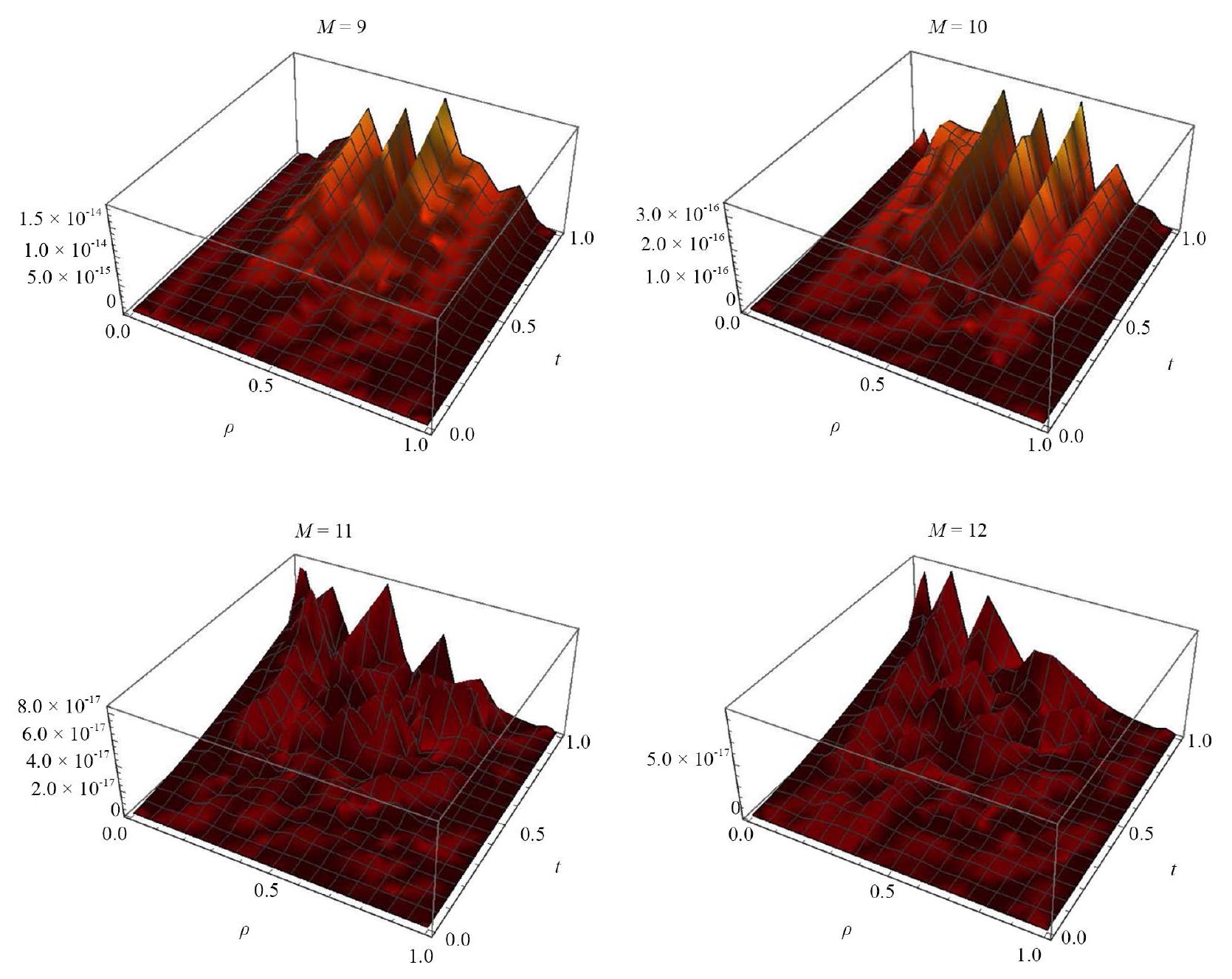
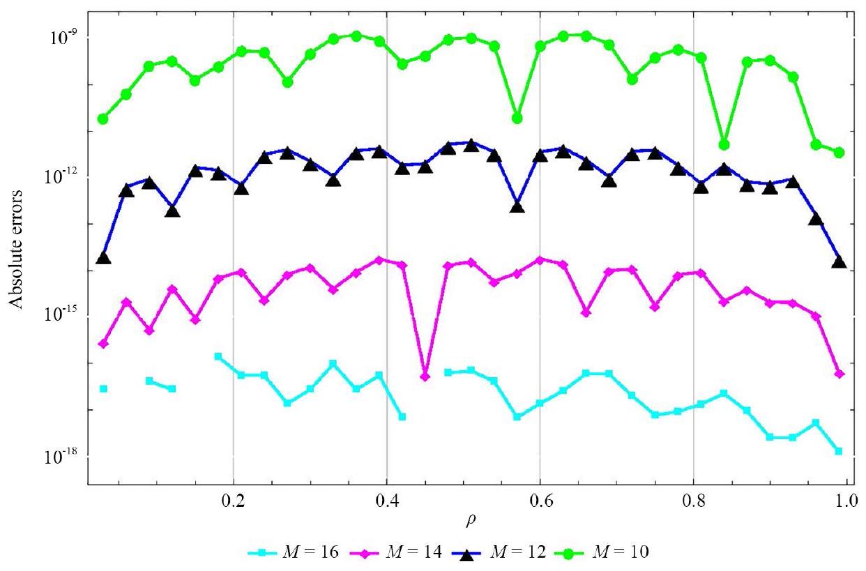
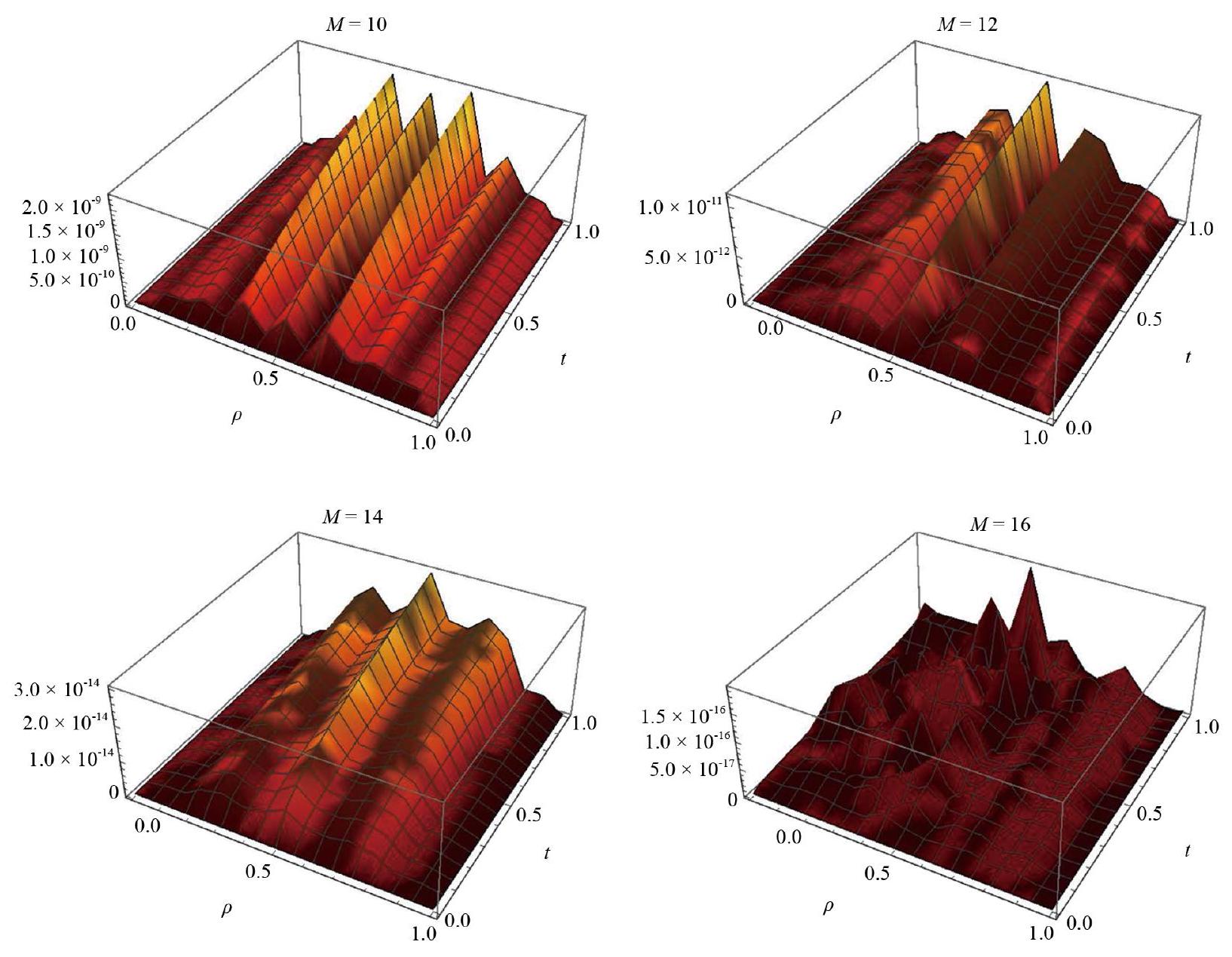
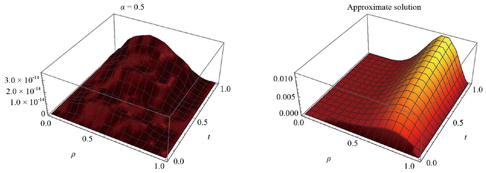
4. Illustrative examples

Example 1 Consider the following TFKdVB equation
subject to
where is the exact solution of equations (50) and (51) and is determined by equation (50) compatible with the solution chosen.
The absolute errors (AE) obtained via the suggested method are shown in Table 1 when and indicating that it is effective in providing a highly precise approximation of the exact solution. The AE for various values of at are shown in Figure 1. This figure verifies that the suggested approach reduces errors consistently throughout the domain and shows a good agreement of the approximate solution with the exact one. The errors at various values when and are shown in Table 2.
Table 1. The AE of Example 1 at
0.1
0.2
0.3
0.4
0.5 0 0
0.6
0.7
0.8
0.9 0
Figure 1. The AE of Example 1 at different values of when
Table 2. The errors of Example 1 at when
0.1
0.2
0.3
0.4
0.5
0.6
0.7
0.8
0.9
Example 2 [32-34] Consider the following TFKdVB equation
subject to
where is the exact solution of equations (52) and (53) and is determined by equation (52) consistent with the chosen solution.
A comparison of the error at and between present technique and the method in [32] is shown in Table 3. A comparison of the at at various values of between current technique and the method in [33] is shown in Table 4. A comparison of the maximum errors at between current technique and the method in [34] is shown in Table 5. We see in these tables that the results are accurate for small choices of . Also, these comparisons reveal the superior performance of our technique over methods in [32-34]. When and , the AE is displayed for various values in Figure 2. The approximate and exact solutions at and is shown in Figure 3. When , the AE is shown at various values in Figure 4. Lastly, for and , Table 6 displays the errors at various values of .
Table 3. Comparison of errors of Example 2
0.4 0.8
Method in [32] at
Method in [32] at
Our method at
Table 4. Comparison of errors of Example 2
0.25 0.5 0.75
Method in [33] at
Our method at
Table 5. Comparison of maximum errors of Example 2 at
Method in [34] at Our method at
0.25
0.125
0.0625
Figure 2. The AE for Example 2 at different values of for and
Figure 3. The approximate and exact solutions for Example 2 at and
Table 6. The errors of Example 2 at when
0.4
0.8
0.9
Figure 4. The AE of Example 2 at different values of when
Example 3 Consider the following TFKdVB equation
subject to
where is the exact solution of equations (54) and (55) and is determined by equation (54) consistent with the chosen solution.
Figure 5. The AE (left) at and approximate solution (right) for Example 3 when
Figure 6. The AE at different values of for Example 3 when
When and , the errors at various values of are shown in Table 7. The AE (left) and approximate solution (right) for when are shown in Figure 5. This figure verifies that the suggested approach reduces errors consistently throughout the domain and shows a good agreement of the approximate solution with the exact one.
Finally, AE at different values of when is shown in Figure 6. These results show a good agreement of the approximate solution with the exact one.
Table 7. The errors of Example 3 at when
0.1
0.2
0.3
0.4
0.5
0.6
0.7
0.8
0.9

5. Concluding remarks

We created a numerical method using the collocation technique to solve the TFKdVB problem. Shifted Chebyshev polynomials may effectively handle fractional derivatives in both space and temporal dimensions. The scheme for solving fractional partial differential equations is efficient and accurate, as demonstrated by numerical experiments. Further research could apply this approach to more complex equations with higher-order derivatives or non-linear terms. This method could be extended to more complicated equations with non-linear components or higher-order derivatives in future studies. Investigating linked systems of time-fractional equations, where the interplay of several equations presents extra difficulties, is a possible extension of this work. To further investigate the method’s resilience and adaptability, it might be modified for three-dimensional situations or equations with stochastic terms. Lastly, hybrid approaches that integrate machine learning techniques with this collocation methodology may present interesting paths toward increasing accuracy and speeding up calculations in large-scale applications.

Conflict of interest

The authors declare no competing financial interest.

References

[1] Korteweg DJ, De Vries G. On the change of form of long waves advancing in a rectangular channel, and a new type of long stationary wave. Philosophical Magazine. 1895; 39: 422-443.
[2] Su CH, Gardner CS. Korteweg-de Vries equation and generalizations III. Derivation of the Korteweg-de Vries equation and Burgers equation. Journal of Mathematical Physics. 1969; 10(3): 536-539. Available from: https: //doi.org/10.1063/1.1664873.
[3] Wang Q. Homotopy perturbation method for fractional KdV-Burgers equation. Chaos, Solitons & Fractals. 2008; 35(5): 843-850. Available from: https://doi.org/10.1016/j.chaos.2006.05.074.
[4] Golmankhaneh AK, Baleanu D. Homotopy perturbation method for solving a system of Schrödinger-Korteweg-de Vries equations. Romanian Reports in Physics. 2011; 63(3): 609-623.
[5] Bhrawy AH, Zaky MA, Baleanu D. New numerical approximations for space-time fractional Burgers’ equations via a Legendre spectral-collocation method. Romanian Reports in Physics. 2015; 67: 340-349.
[6] Atta AG, Abd-Elhameed WM, Moatimid GM, Youssri YH. Novel spectral schemes to fractional problems with nonsmooth solutions. Mathematical Methods in the Applied Sciences. 2023; 46(13): 14745-14764. Available from: https://doi.org/10.1002/mma.9343.
[7] Bose CSV, Udhayakumar R, Muthukumaran V, Al-Omari S. A study on approximate controllability of Ψ-Caputo fractional differential equations with impulsive effects. Contemporary Mathematics. 2024; 5(1): 175-198. Available from: https://doi.org/10.37256/cm.5120243539.
[8] Bose CSV, Udhayakumar R. Approximate controllability of -Caputo fractional differential equation. Mathematical Methods in the Applied Sciences. 2023; 46(17): 17660-17671. Available from: https://doi.org/10.1002/mma.9523.
[9] Atta AG, Youssri YH. Shifted second-kind Chebyshev spectral collocation-based technique for time-fractional KdV-Burgers’ equation. Iranian Journal of Mathematical Chemistry. 2023; 14(4): 207-224. Available from: https: //doi.org/10.22052/ijmc.2023.252824.1710.
[10] Inc M, Parto-Haghighi M, Akinlar MA, Chu YM. New numerical solutions of fractional-order Korteweg-de Vries equation. Results in Physics. 2020; 19: 103326. Available from: https://doi.org/10.1016/j.rinp.2020.103326.
[11] Shi Y, Xu B, Guo Y. Numerical solution of Korteweg-de Vries-Burgers equation by the compact-type CIP method. Advances in Difference Equations. 2015; 2015: 1-9. Available from: https://doi.org/10.1186/s13662-015-0682-5.
[12] Yousif MA, Guirao JL, Mohammed PO, Chorfi N, Baleanu D. A computational study of time-fractional gas dynamics models by means of conformable finite difference method. AIMS Mathematics. 2024; 9(7): 19843-19858. Available from: https://doi.org/10.3934/math.2024969.
[13] Yousif MA, Hamasalh FK. Conformable non-polynomial spline method: A robust and accurate numerical technique. Ain Shams Engineering Journal. 2024; 15(2): 102415. Available from: https://doi.org/10.1016/j.asej.2023.102415.
[14] Mohammed PO, Agarwal RP, Brevik I, Abdelwahed M, Kashuri A, Yousif MA. On multiple-type wave solutions for the nonlinear coupled time-fractional Schrödinger model. Symmetry. 2024; 16(5): 553. Available from: https: //doi.org/10.3390/sym16050553.
[15] Abd-Elhameed WM, Youssri HY, Atta AG. Tau algorithm for fractional delay differential equations utilizing seventhkind Chebyshev polynomials. Journal of Mathematical Modeling. 2024; 12(2): 277-299. Available from: https: //doi.org/10.22124/jmm.2024.25844.2295.
[16] Youssri HY, Atta AG. Modal spectral Tchebyshev Petrov-Galerkin stratagem for the time-fractional nonlinear Burgers’ equation. Iranian Journal of Numerical Analysis and Optimization. 2024; 14(1): 172-199. Available from: https://doi.org/10.22067/ijnao.2023.83389.1292.
[17] Youssri YH, Ismail MI, Atta AG. Chebyshev Petrov-Galerkin procedure for the time-fractional heat equation with nonlocal conditions. Physica Scripta. 2023; 99(1): 015251. Available from: https://doi.org/10.1088/1402-4896/ ad1700.
[18] Youssri YH, Atta AG, Moustafa MO, Abu Waar ZY. Explicit collocation algorithm for the nonlinear fractional Duffing equation via third-kind Chebyshev polynomials. Iranian Journal of Numerical Analysis and Optimization. 2025; 2025: 1543. Available from: https://doi.org/10.22067/ijnao.2025.90483.1543.
[19] Hughes TJR. The Finite Element Method: Linear Static and Dynamic Finite Element Analysis. New York: Dover Publications; 2012.
[20] Boyd JP. Spectral Methods for Partial Differential Equations. Philadelphia, Pennsylvania, United States: SIAM; 2001.
[21] Atta AG, Soliman JF, Elsaeed EW, Elsaeed MW, Youssri YH. Spectral collocation algorithm for the fractional Bratu equation via hexic shifted Chebyshev polynomials. Computational Methods for Differential Equations. 2024; 2024: 2621. Available from: https://doi.org/10.22034/cmde.2024.61045.2621.
[22] Atta AG, Abd-Elhameed WM, Youssri YH. Approximate collocation solution for the time-fractional Newell-Whitehead-Segel equation. Journal of Applied and Computational Mechanics. 2024; 2024: 4686. Available from: https://doi.org/10.22055/jacm.2024.47269.4686.
[23] Abd-Elhameed WM, Ahmed HM, Zaky MA, Hafez RM. A new shifted generalized Chebyshev approach for multidimensional sinh-Gordon equation. Physica Scripta. 2024; 99(9): 095269. Available from: https://dx.doi.org/10. 1088/1402-4896/ad6fe3.
[24] Ahmed HM, Abd-Elhameed WM. Spectral solutions of specific singular differential equations using a unified spectral Galerkin-collocation algorithm. Journal of Nonlinear Mathematical Physics. 2024; 31(1): 42. Available from: https://doi.org/10.1007/s44198-024-00194-0.
[25] Ahmed HM, Hafez RM, Abd-Elhameed WM. A computational strategy for nonlinear time-fractional generalized Kawahara equation using new eighth-kind Chebyshev operational matrices. Physica Scripta. 2024; 99(4): 045250. Available from: https://dx.doi.org/10.1088/1402-4896/ad3482.
[26] Abd-Elhameed WM, Ahmed HM. Spectral solutions for the time-fractional heat differential equation through a novel unified sequence of Chebyshev polynomials. AIMS Mathematics. 2024; 9(1): 2137-2166. Available from: https://doi.org/10.3934/math.2024107.
[27] Abdelghany EM, Abd-Elhameed WM, Moatimid GM, Youssri HY, Atta AG. A Tau approach for solving timefractional heat equation based on the shifted sixth-kind Chebyshev polynomials. Symmetry. 2023; 15(3): 594. Available from: https://doi.org/10.3390/sym15030594.
[28] Podlubny I. Fractional Differential Equations. PA, USA: Elsevier; 1998.
[29] Youssri YH, Atta AG. Double TChebyshev spectral tau algorithm for solving KdV equation, with soliton application. In: Solitons. New York, NY: Springer; 2022. p.451-467. Available from: https://doi.org/10.1007/ 978-1-0716-2457-9_771.
[30] Abd-Elhameed WM, Machado JAT, Youssri YH. Hypergeometric fractional derivatives formula of shifted Chebyshev polynomials: tau algorithm for a type of fractional delay differential equations. International Journal of Nonlinear Sciences and Numerical Simulation. 2022; 23(7-8): 1253-1268. Available from: https://doi.org/10.1515/ ijnsns-2020-0124.
[31] Askey R. Orthogonal Polynomials and Special Functions. PA, USA: SIAM; 1975.
[32] Cen D, Wang Z, Mo Y. Second order difference schemes for time-fractional KdV-Burgers’ equation with initial singularity. Applied Mathematics Letters. 2021; 112: 106829. Available from: https://doi.org/10.1016/j.aml.2020. 106829.
[33] Karaagac B, Esen A, Owolabi KM, Pindza E. A collocation method for solving time fractional nonlinear Kortewegde Vries-Burgers equation arising in shallow water waves. International Journal of Modern Physics C. 2023; 34(7): 2350096. Available from: https://doi.org/10.1142/S0129183123500961.
[34] Vivas-Cortez M, Yousif MA, Mahmood BA, Mohammed PO, Chorfi N, Lupas AA. High-accuracy solutions to the time-fractional KdV-Burgers equation using rational non-polynomial splines. Symmetry. 2024; 17(1): 16. Available from: https://doi.org/10.3390/sym17010016.

  1. Copyright (C)2025 Laila A. Alnaser, et al.
    DOI: https://doi.org/10.37256/cm. 6220255948
    This is an open-access article distributed under a CC BY license
    (Creative Commons Attribution 4.0 International License)
    https://creativecommons.org/licenses/by/4.0/