DOI: https://doi.org/10.1007/s13042-024-02110-w
تاريخ النشر: 2024-03-05
نهج مبتكر لتحويل سوان يستخدم الشبكة العصبية متعددة الطبقات المتبقية لتشخيص أورام الدماغ في صور الرنين المغناطيسي
© المؤلفون 2024
الملخص
تتطلب العواقب الخطيرة الناتجة عن أورام الدماغ تشخيصًا دقيقًا وفي الوقت المناسب. ومع ذلك، فإن العقبات مثل جودة التصوير غير المثلى، ومشاكل سلامة البيانات، وأنواع الأورام ومراحلها المتنوعة، والأخطاء المحتملة في التفسير تعيق تحقيق تشخيصات دقيقة وسريعة. يلعب التعرف السريع على أورام الدماغ دورًا محوريًا في ضمان سلامة المرضى. أنظمة التعلم العميق تحمل وعدًا في مساعدة أطباء الأشعة على إجراء التشخيصات بسرعة ودقة. في هذه الدراسة، نقدم نهجًا متقدمًا للتعلم العميق يعتمد على محول سوين. الطريقة المقترحة تقدم وحدة جديدة من الانتباه الذاتي متعدد الرؤوس مع نوافذ هجينة (HSW-MSA) جنبًا إلى جنب مع نموذج معاد قياسه. يهدف هذا التحسين إلى تحسين دقة التصنيف، وتقليل استخدام الذاكرة، وتبسيط تعقيد التدريب. تستبدل شبكة MLP المعتمدة على المتبقي (ResMLP) شبكة MLP التقليدية في محول سوين، مما يحسن الدقة وسرعة التدريب وكفاءة المعلمات. نقوم بتقييم نموذج Proposed-Swin على مجموعة بيانات الرنين المغناطيسي للدماغ المتاحة للجمهور مع أربع فئات، باستخدام بيانات الاختبار فقط. يتم تعزيز أداء النموذج من خلال تطبيق تقنيات التعلم الانتقالي وزيادة البيانات لتدريب فعال وقوي. يحقق نموذج Proposed-Swin دقة ملحوظة تبلغ
1 المقدمة
أطباء الأشعة [6، 7، 13، 14]. في مجال تشخيص أورام الدماغ، بذل الباحثون جهودًا كبيرة لتقليل المراضة والوفيات المرتبطة بها [11]. تقليديًا، أثبت الكشف اليدوي عن أورام الدماغ من قبل أطباء الأشعة أنه عبء بسبب الصور العديدة المعنية. أصبحت أنظمة التشخيص المدعومة بالكمبيوتر (CADx) أدوات مفيدة للتغلب على هذه الصعوبة من خلال أتمتة وتبسيط الإجراء التشخيصي [15]. أظهرت أنظمة CADx المعتمدة على التعلم العميق معدلات نجاح ملحوظة في تحليل الصور الطبية، وتشخيص السرطان، بما في ذلك أورام الدماغ وأنواع السرطان الأخرى [16-21]. لا تساعد هذه الأنظمة فقط في اكتشاف الأورام ومراقبتها، ولكنها تساعد أيضًا الأطباء في اتخاذ قرارات بشأن خيارات العلاج المناسبة، مما يحسن في النهاية رعاية المرضى [22-24].
[37]. ومع ذلك، لا يزال هناك حاجة إلى تحسين مستمر من حيث الدقة والكفاءة والوصول في تشخيص وإدارة أورام الدماغ. تحمل الأبحاث والابتكارات المستمرة وعدًا بإحداث ثورة في هذا المجال من خلال تقديم تقنيات وأدوات أكثر فعالية لتشخيص أورام الدماغ، مما يؤدي في النهاية إلى تحسين النتائج للمرضى. لقد كانت فعالية طرق التعلم العميق في تشخيص أنواع مختلفة من السرطان دافعًا للباحثين في هذا المجال [38].
- قمنا بتطوير نموذج من خلال توسيع بنية Swin بناءً على نموذج Swin-Base لمجموعة من صور الرنين المغناطيسي للدماغ من 4 فئات. يوفر هذا النموذج الموسع دقة كشف محسّنة مع عدد أقل من المعلمات في نفس الوقت وهو أقل عمقًا من نماذج Swin السابقة.
- يحسن النموذج المقترح Swin Transformer من خلال تقديم وحدة الانتباه الذاتي الهجينة ذات النوافذ المتداخلة (HSW-MSA)، مما يمكّن من معالجة أفضل لمناطق الرنين المغناطيسي للدماغ المتداخلة. يسمح هذا التحسين للنموذج بالتقاط التفاصيل الدقيقة والاعتماديات بعيدة المدى بشكل أكثر فعالية، مما يؤدي إلى تحسين الدقة في اكتشاف أورام الدماغ وتقليل النتائج السلبية الكاذبة.
- علاوة على ذلك، تستبدل الورقة متعددة الطبقات (MLP) في Swin Transformer بـ MLP قائم على المتبقي (ResMLP). تؤدي هذه التغييرات المعمارية إلى دقة أعلى، وتدريب أسرع، وكفاءة محسّنة في المعلمات. تساهم قدرة ResMLP على استخراج وتمثيل الميزات بشكل أكثر كفاءة في الأداء الاستثنائي لنموذج Proposed-Swin على مجموعة بيانات الرنين المغناطيسي للدماغ.
- تظهر التقييمات الشاملة دقة استثنائية قدرها
التي حققها نموذج Proposed-Swin، متجاوزة الأبحاث الحالية ونماذج التعلم العميق. تسلط هذه الفعالية الملحوظة الضوء على إمكاناتها للتطبيق العملي في البيئات الواقعية لتشخيص أورام الدماغ بدقة. - بالإضافة إلى ذلك، أظهرنا فعالية نماذج المحولات البصرية الحالية والمحبوبة ونماذج CNN باستخدام مجموعات بيانات الرنين المغناطيسي المتاحة علنًا لتقديم مقارنة شاملة.
2 الأعمال ذات الصلة
3 المواد والأساليب
3.1 مجموعة البيانات
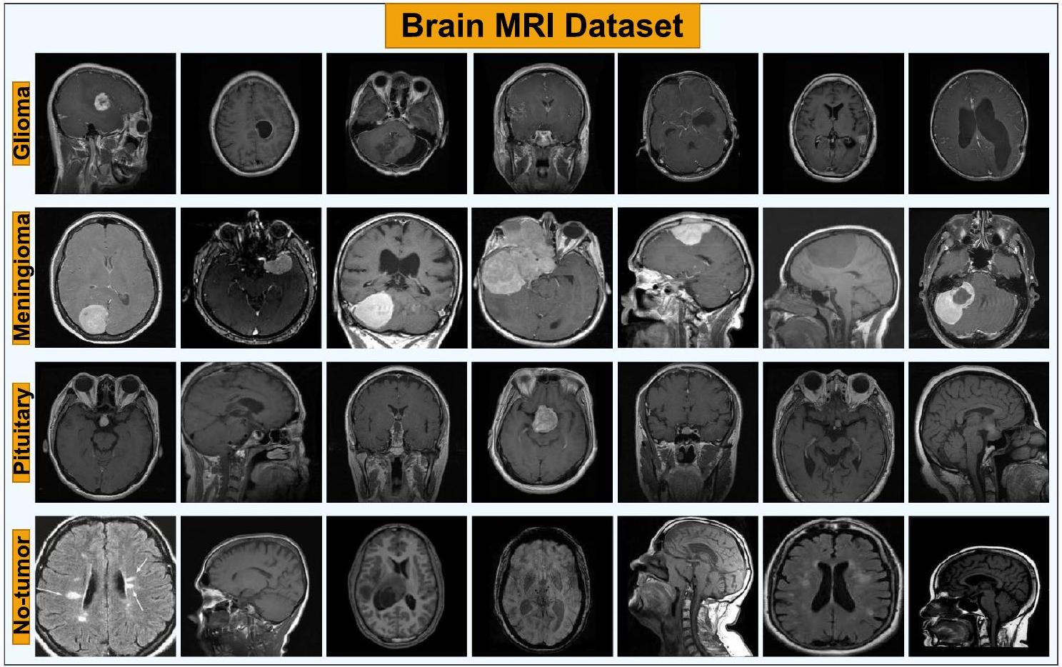
وإجراء توقعات دقيقة على البيانات غير المرصودة مع مجموعة بيانات كبيرة وتمثيلية. إن ضمان جودة البيانات العالية أمر ضروري لمعالجة التحيزات، وتقليل مشاكل التكيف الزائد أو الناقص، وتحسين الأداء عبر مجموعات فرعية مختلفة. من أجل التصنيف الذاتي لصور الرنين المغناطيسي منخفضة الدرجة، توجد عدة مجموعات بيانات متاحة للجمهور، بما في ذلك Figshare [53] وSARTAJ [54] وBr35H [55]، والتي تُعرف بأنها مجموعات بيانات صغيرة الحجم. ومع ذلك، في هذه الدراسة، استخدمنا مجموعة بيانات الرنين المغناطيسي للدماغ المتاحة للجمهور والتي تم مشاركتها على Kaggle [56]، والتي تجمع وتدمج هذه المجموعات الثلاث لإظهار القدرات الحقيقية لنماذج التعلم العميق في هذه المهمة. يتم توضيح صور عينة من هذه المجموعة التي تصور كل من حالات الورم والحالات الصحية في الشكل 1.
3.2 محول الرؤية
3.3 محول سوين
تُجمع الميزات للحصول على متجه ميزات بأبعاد 4C، والذي يتم تحويله باستخدام طبقات خطية مع الحفاظ على دقة
أين
3.4 النموذج المقترح
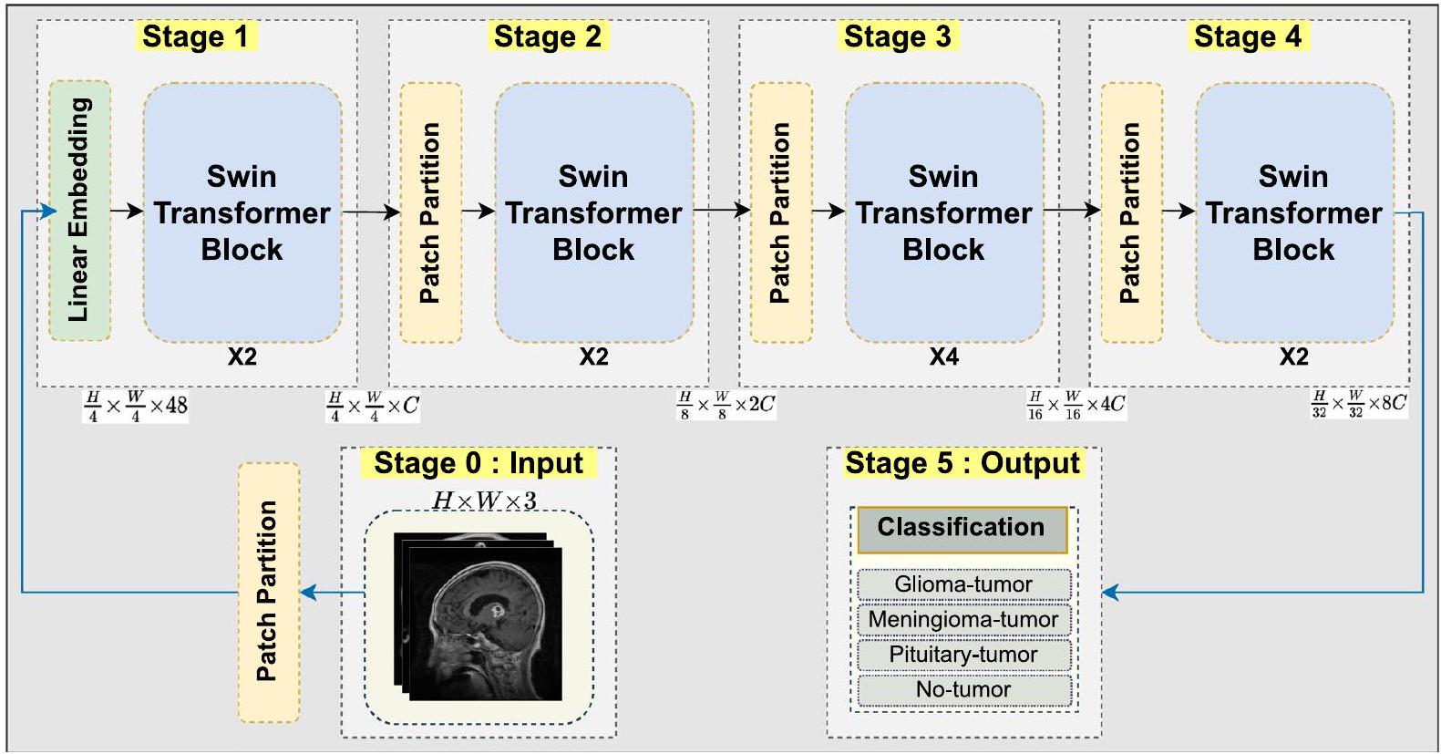
يحتاج إلى تعديل تصميمه ومعاييره لاستيعاب مجموعة متنوعة من أحمال العمل وأحجام مجموعات البيانات. يمكن أن تساعد متغيرات مثل حجم النموذج، وعمق المرحلة، وأبعاد التضمين في تحقيق ذلك. على سبيل المثال، توفر التغييرات الأكبر من Swin Transformer، مثل Swin-Base وSwin-Large، المصممة لمجموعات بيانات مثل ImageNet التي تحتوي على 1000 فئة، سعة محسّنة مناسبة للتعامل مع المهام الأكثر صعوبة ومجموعات البيانات الأكبر. من ناحية أخرى، تنتج نماذج Swin-Small وSwin-Tiny نتائج أكثر فائدة في السيناريوهات التي تحتوي على فئات أقل مع استخدام موارد أقل للمهام الأبسط. يتم توضيح التصميم العام لنموذج Proposed-Swin Transformer لاكتشاف أورام الدماغ في الشكل 2.
3.4.1 وحدة الانتباه الذاتي الهجين المتعدد
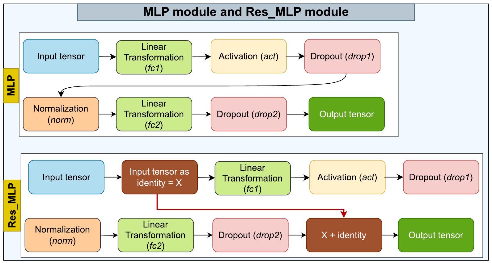
مع أشكال مستطيلة ممدودة في الاتجاهات الأفقية والعمودية. على عكس كتل المحولات التقليدية، التي تستخدم آليات الانتباه الذاتي المتصلة بالكامل، يسمح هذا الوحدة الهجينة للنموذج بالتقاط المعلومات بشكل مرن من نوافذ بأحجام مختلفة، مما يعالج الاعتماديات بعيدة المدى مع الحفاظ على المعلومات المحلية والتفصيلية. تعزز القدرة على التعامل مع الصور بمقاييس واتجاهات مختلفة من قابلية تطبيق النموذج وتقلل من مشكلات التعميم، مما قد يؤدي إلى تحسين الأداء في مهام تحليل الصور الصعبة مثل اكتشاف أورام الدماغ وصور طبية أخرى. توضح الشكل 3 كتلة المحول النقي Swin جنبًا إلى جنب مع كتل المحولات الهجينة المستخدمة في النموذج المقترح.
أين
3.4.2 وحدة الشبكة العصبية المتعددة الطبقات المتبقية (Res-MLP)
4 النتائج والمناقشات
4.1 تصميم التجربة
4.2 معالجة البيانات وتعلم النقل
مع الآخرين، استخدمنا
4.3 مقاييس الأداء
| اسم الفصل | قطار | التحقق | اختبار | إجمالي |
| ورم الدبقيات | ١٠٥٧ | 264 | ٣٠٠ | 1,621 |
| ورم السحايا | 1072 | 267 | 306 | 1,645 |
| ورم الغدة النخامية | 1166 | 291 | ٣٠٠ | 1,757 |
| لا ورم | 1276 | ٣١٩ | ٤٠٥ | ٢٬٠٠٠ |
| إجمالي | 4571 | 1141 | 1,311 | ٧٠٢٣ |
4.4 إجراء التدريب
| مقياس | صيغة |
| دقة |
|
| دقة |
|
| استدعاء |
|
| درجة F1 |
|
4.5 النتائج
| نموذج | دقة | دقة | استدعاء | درجة F1 |
| VGG16 [67] | 0.9924 | 0.9921 | 0.9917 | 0.9917 |
| ResNet50 [63] | 0.9893 | 0.9887 | 0.9886 | 0.9886 |
| EfficientNetv2-متوسط [68] | 0.9924 | 0.9919 | 0.9917 | 0.9917 |
| MobileNetv3-صغير [69] | 0.9939 | 0.9936 | 0.9934 | 0.9935 |
| MobileViT-صغير [70] | 0.9947 | 0.9942 | 0.9942 | 0.9942 |
| MobileViTv2-150 [71] | 0.9954 | 0.9953 | 0.9950 | 0.9952 |
| ماكس فيت-بيس [72] | 0.9931 | 0.9926 | 0.9927 | 0.9927 |
| ديت-بيس [73] | 0.9947 | 0.9943 | 0.9942 | 0.9942 |
| DeiT3-Base [74] | 0.9924 | 0.9919 | 0.9919 | 0.9919 |
| في تي-بيس-باتش32 [57] | 0.9939 | 0.9934 | 0.9934 | 0.9934 |
| بي تي-بيس [75] | 0.9954 | 0.9951 | 0.9950 | 0.9950 |
| كونفيت-بيس [76] | 0.9931 | 0.9928 | 0.9925 | 0.9926 |
| توأم-سفط-قاعدة [77] | 0.9924 | 0.9918 | 0.9924 | 0.9921 |
| بي تي-بيس [78] | 0.9947 | 0.9943 | 0.9942 | 0.9942 |
| سوين-تايني [60] | 0.9931 | 0.9927 | 0.9925 | 0.9926 |
| سوينف2-ويندوز16-صغير [61] | 0.9939 | 0.9935 | 0.9933 | 0.9934 |
| GcViT-Base [79] | 0.9947 | 0.9944 | 0.9942 | 0.9942 |
| سوين المقترح | 0.9992 | 0.9992 | 0.9992 | 0.9992 |
التنفيذ العملي في أنظمة التصوير الطبي والتشخيص. من بين النماذج التي تم تقييمها، يبرز نموذج Proposed-Swin بنتائج استثنائية، حيث حقق مقياسًا ممتازًا قدره 0.9992. وهذا يدل على أن نموذج Proposed-Swin فعال للغاية في تصنيف صور الرنين المغناطيسي للدماغ بدقة، مما يجعله مرشحًا واعدًا للتطبيقات السريرية في العالم الحقيقي.
(المقترح-Swin)، يليه MobileViTv2-150، BeiTBase، MobileViT-Small، DeiT-Base، حيث أن ResNet50 هو أقل نموذج أداءً. ومن الجدير بالذكر أن النموذج الحالي، DeiT3، يظهر أداءً أقل مقارنة بسلفه، نموذج DeiT. وهذا يبرز التباين في الأداء الذي يمكن أن يظهره كل نموذج على مجموعات البيانات الطبية.
4.6 كفاءة نموذج سوين المقترح وبدائل محول سوين
نافذة متغيرة. إنها تخصص بشكل استراتيجي
4.7 المقارنة مع الأساليب المتطورة
| نموذج | دقة | دقة | استدعاء | درجة F1 |
| سوين-تايني | 0.9931 | 0.9927 | 0.9925 | 0.9926 |
| سوين-سمول | 0.9939 | 0.9935 | 0.9933 | 0.9934 |
| سوين-بيس | 0.9954 | 0.9951 | 0.9950 | 0.9950 |
| سوين-لارج | 0.9947 | 0.9944 | 0.9942 | 0.9942 |
| سوينف2-ويندوز8-صغير | 0.9962 | 0.9961 | 0.9959 | 0.9960 |
| سوينف2-ويندوز16-صغير | 0.9939 | 0.9935 | 0.9933 | 0.9934 |
| سوينف2-ويندوز8-صغير | 0.9954 | 0.9952 | 0.995 | 0.9951 |
| سوينف2-نافذة16-صغير | 0.9947 | 0.9942 | 0.9942 | 0.9942 |
| سوينف2-ويندوز8-أساسي | 0.9947 | 0.9944 | 0.9942 | 0.9942 |
| سوينف2-ويندوز16-أساسي | 0.9947 | 0.9943 | 0.9942 | 0.9942 |
| سوينف2-نافذة12-كبير | 0.9954 | 0.9953 | 0.995 | 0.9952 |
| سوين المقترح | 0.9992 | 0.9992 | 0.9992 | 0.9992 |
التصنيف، مع التركيز بشكل خاص على المهمة الحيوية لتشخيص أورام الدماغ. وسط مجموعة من المنهجيات المقدمة من دراسات مختلفة، يبرز نموذج Proposed-Swin (ViT) كقمة الأداء في اكتشاف الشذوذات الدماغية. إن تقارب تقنيات الرؤية الحاسوبية المتقدمة والتصوير الطبي واضح بشكل لافت في الدقة الاستثنائية لنموذج Proposed-Swin (ViT) على مجموعة بيانات كاجل، حيث وصلت إلى نسبة مثيرة للإعجاب
4.8 القيود والاتجاهات المستقبلية
المأخوذة من مؤسسات الرعاية الصحية المختلفة لتعزيز أداء نموذج Swin وقابلية تعميمه. يعد هذا التحقق متعدد المراكز أمرًا حيويًا لتقييم أداء النموذج عبر بروتوكولات التصوير المختلفة وخصائص المرضى. بالإضافة إلى ذلك، تهدف الدراسات المخطط لها إلى إظهار أداء النموذج على صور طبية مختلفة. تحسين نموذج Swin للتطبيقات في الوقت الحقيقي هو أيضًا اتجاه مستقبلي مهم. يعد تحسين بنية النموذج واستراتيجيات الاستدلال الفعالة أمرًا أساسيًا لتوفير دعم تشخيصي في الوقت المناسب وفي الموقع للأطباء.
5 الخاتمة
| المؤلف والسنة | مجموعة البيانات | الطريقة | نسبة الدقة % |
| Talukder وآخرون، 2023 [13] | Figshare | معتمد على CNN | 99.68 |
| Tabatabaei وآخرون، 2023 [48] | Figshare | CNN + انتباه | 99.30 |
| ديباك وأمير، 2023 [80] | Figshare | CNN+SVM | 95.60 |
| زلفقار وآخرون، 2023 [32] | Figshare | معتمد على CNN | 98.86 |
| غسمي وآخرون، 2020 [47] | Figshare | CNN+GAN | 95.60 |
| مهنتكش وآخرون، 2023 [33] | Figshare | معتمد على CNN | 98.69 |
| سواتي وآخرون، 2019 [51] | Figshare | معتمد على CNN | 94.82 |
| سجاد وآخرون، 2019 [52] | Figshare | معتمد على CNN | 90.67 |
| رحمن وآخرون، 2020 [42] | Figshare | معتمد على CNN | 98.69 |
| كومار وآخرون، 2021 [41] | Figshare | معتمد على CNN | 97.48 |
| مزوقي وآخرون، 2020 [44] | BraTS | معتمد على CNN | 96.49 |
| شريف وآخرون، 2022 [43] | BraTS | معتمد على CNN | 98.80 |
| أوزكاراكا وآخرون، 2023 [81] | كاجل | معتمد على CNN | 96.00 |
| رحمن وإسلام، 2023 [82] | كاجل | معتمد على CNN | 98.12 |
| موئزين أوغلو وآخرون، 2023 [83] | كاجل | معتمد على CNN | 98.10 |
| علي وآخرون، 2023 [84] | كاجل | معتمد على CNN | 95.70 |
| Proposed-Swin | كاجل | معتمد على Swin (ViT) | 99.92 |
الإعلانات
الموافقة الأخلاقية لم تكن هناك حاجة للحصول على موافقة أخلاقية لهذا العمل لأنه لم يتضمن أشخاصًا بشريين، أو حيوانات، أو بيانات حساسة تتطلب مراجعة أخلاقية.
References
- Bondy ML, Scheurer ME, Malmer B et al (2008) Brain tumor epidemiology: consensus from the Brain Tumor Epidemiology Consortium. Cancer 113:1953-1968
- Herholz K, Langen KJ, Schiepers C, Mountz JM (2012) Brain tumors. Semin Nucl Med 42:356-370. https://doi.org/10.1053/j. semnuclmed.2012.06.001
- Ostrom QT, Barnholtz-Sloan JS (2011) Current state of our knowledge on brain tumor epidemiology. Curr Neurol Neurosci Rep 11:329-335. https://doi.org/10.1007/s11910-011-0189-8
- Miller KD, Ostrom QT, Kruchko C et al (2021) Brain and other central nervous system tumor statistics, 2021. CA Cancer J Clin 71:381-406. https://doi.org/10.3322/caac. 21693
- Charles NA, Holland EC, Gilbertson R et al (2011) The brain tumor microenvironment. Glia 59:1169-1180. https://doi.org/10. 1002/glia. 21136
- Liu Z, Tong L, Chen L et al (2023) Deep learning based brain tumor segmentation: a survey. Complex Intell Syst 9:1001-1026. https://doi.org/10.1007/s40747-022-00815-5
- Jyothi P, Singh AR (2023) Deep learning models and traditional automated techniques for brain tumor segmentation in MRI: a review. Artif Intell Rev 56:2923-2969. https://doi.org/10.1007/ s10462-022-10245-x
- Solanki S, Singh UP, Chouhan SS, Jain S (2023) Brain tumor detection and classification using intelligence techniques: an overview. IEEE Access 11:12870-12886
- Villanueva-Meyer JE, Mabray MC, Cha S (2017) Current clinical brain tumor imaging. Clin Neurosurg 81:397-415. https://doi.org/ 10.1093/neuros/nyx103
- Ellingson BM, Wen PY, Van Den Bent MJ, Cloughesy TF (2014) Pros and cons of current brain tumor imaging. Neuro Oncol 16:vii2-vii11. https://doi.org/10.1093/neuonc/nou224
- Xie Y, Zaccagna F, Rundo L et al (2022) Convolutional neural network techniques for brain tumor classification (from 2015 to 2022): review, challenges, and future perspectives. Diagnostics 12:1850
- Ali S, Li J, Pei Y et al (2022) A comprehensive survey on brain tumor diagnosis using deep learning and emerging hybrid techniques with multi-modal MR image. Arch Comput Methods Eng 29:4871-4896
- Talukder MA, Islam MM, Uddin MA et al (2023) An efficient deep learning model to categorize brain tumor using reconstruction and fine-tuning. Expert Syst Appl. https://doi.org/10.1016/j. eswa.2023.120534
- Rajeev SK, Pallikonda Rajasekaran M, Vishnuvarthanan G, Arunprasath T (2022) A biologically-inspired hybrid deep learning approach for brain tumor classification from magnetic resonance imaging using improved gabor wavelet transform and Elmann-BiLSTM network. Biomed Signal Process Control. https://doi.org/10.1016/j.bspc.2022.103949
- Pacal I, Kılıcarslan S (2023) Deep learning-based approaches for robust classification of cervical cancer. Neural Comput Appl. https://doi.org/10.1007/s00521-023-08757-w
- Coşkun D, Karaboğa D, Baştürk A et al (2023) A comparative study of YOLO models and a transformer-based YOLOv5 model for mass detection in mammograms. Turk J Electr Eng Comput Sci 31:1294-1313. https://doi.org/10.55730/13000632.4048
- Wang W, Pei Y, Wang SH et al (2023) PSTCNN: explainable COVID-19 diagnosis using PSO-guided self-tuning CNN. Biocell 47:373-384. https://doi.org/10.32604/biocell.2023.025905
- Pacal I, Karaboga D (2021) A robust real-time deep learning based automatic polyp detection system. Comput Biol Med. https://doi. org/10.1016/j.compbiomed.2021.104519
- Zhang Y-D, Govindaraj VV, Tang C et al (2019) High performance multiple sclerosis classification by data augmentation and AlexNet transfer learning model. J Med Imaging Health Inform 9:2012-2021. https://doi.org/10.1166/JMIHI.2019.2692
- Wang W, Zhang X, Wang SH, Zhang YD (2022) COVID-19 diagnosis by WE-SAJ. Syst Sci Control Eng 10:325-335. https://doi. org/10.1080/21642583.2022.2045645
- Pacal I (2022) Deep learning approaches for classification of breast cancer in ultrasound (US) images. J Inst Sci Technol. https://doi.org/10.21597/jist. 1183679
- Amin J, Sharif M, Haldorai A et al (2022) Brain tumor detection and classification using machine learning: a comprehensive survey. Complex Intell Syst 8:3161-3183. https://doi.org/10.1007/ s40747-021-00563-y
- Deepak S, Ameer PM (2019) Brain tumor classification using deep CNN features via transfer learning. Comput Biol Med. https://doi.org/10.1016/j.compbiomed.2019.103345
- Wang SH, Govindaraj VV, Górriz JM et al (2021) Covid-19 classification by FGCNet with deep feature fusion from graph convolutional network and convolutional neural network. Inform Fusion 67:208-229. https://doi.org/10.1016/j.inffus.2020.10.004
- Chahal PK, Pandey S, Goel S (2020) A survey on brain tumor detection techniques for MR images. Multimed Tools Appl 79:21771-21814. https://doi.org/10.1007/s11042-020-08898-3
- Amin J, Sharif M, Yasmin M, Fernandes SL (2018) Big data analysis for brain tumor detection: deep convolutional neural networks. Futur Gener Comput Syst 87:290-297. https://doi.org/10. 1016/j.future.2018.04.065
- Esmaeili M, Vettukattil R, Banitalebi H et al (2021) Explainable artificial intelligence for human-machine interaction in brain tumor localization. J Pers Med. https://doi.org/10.3390/jpm11 111213
- Zhang Y, Deng L, Zhu H et al (2023) Deep learning in food category recognition. Inform Fusion. https://doi.org/10.1016/j.inffus. 2023.101859
- Karaman A, Karaboga D, Pacal I et al (2022) Hyper-parameter optimization of deep learning architectures using artificial bee colony (ABC) algorithm for high performance real-time automatic colorectal cancer (CRC) polyp detection. Appl Intell. https://doi. org/10.1007/s10489-022-04299-1
- Pacal I, Karaman A, Karaboga D et al (2022) An efficient realtime colonic polyp detection with YOLO algorithms trained by using negative samples and large datasets. Comput Biol Med. https://doi.org/10.1016/J.COMPBIOMED.2021.105031
- Pacal I, Alaftekin M (2023) Türk İşaret Dilinin Sınıflandırılması için Derin Öğrenme Yaklaşımları. Iğdır Üniversitesi Fen Bilimleri Enstitüsü Dergisi 13:760-777. https://doi.org/10.21597/jist. 12234 57
- Zulfiqar F, Ijaz Bajwa U, Mehmood Y (2023) Multi-class classification of brain tumor types from MR images using EfficientNets. Biomed Signal Process Control. https://doi.org/10.1016/j.bspc. 2023.104777
- Mehnatkesh H, Jalali SMJ, Khosravi A, Nahavandi S (2023) An intelligent driven deep residual learning framework for brain tumor classification using MRI images. Expert Syst Appl. https:// doi.org/10.1016/j.eswa.2022.119087
- Shamshad F, Khan S, Zamir SW et al (2023) Transformers in medical imaging: a survey. Med Image Anal 88:102802
- Akinyelu AA, Zaccagna F, Grist JT et al (2022) Brain tumor diagnosis using machine learning, convolutional neural networks, capsule neural networks and vision transformers, applied to MRI: a survey. J Imaging 8:205
- Celard P, Iglesias EL, Sorribes-Fdez JM et al (2023) A survey on deep learning applied to medical images: from simple artificial neural networks to generative models. Neural Comput Appl 35:2291-2323
- Tummala S, Kadry S, Bukhari SAC, Rauf HT (2022) Classification of brain tumor from magnetic resonance imaging using vision transformers ensembling. Curr Oncol 29:7498-7511. https://doi. org/10.3390/curroncol29100590
- Karaman A, Pacal I, Basturk A et al (2023) Robust real-time polyp detection system design based on YOLO algorithms by optimizing activation functions and hyper-parameters with artificial bee colony (ABC). Expert Syst Appl. https://doi.org/10.1016/j.eswa. 2023.119741
- Nazir M, Shakil S, Khurshid K (2021) Role of deep learning in brain tumor detection and classification (2015 to 2020): a review. Comput Med Imaging Graph. https://doi.org/10.1016/j.compm edimag.2021.101940
- Jiang Y, Zhang Y, Lin X et al (2022) SwinBTS: a method for 3D multimodal brain tumor segmentation using Swin transformer. Brain Sci. https://doi.org/10.3390/brainsci12060797
- Kumar RL, Kakarla J, Isunuri BV, Singh M (2021) Multi-class brain tumor classification using residual network and global average pooling. Multimed Tools Appl 80:13429-13438. https://doi. org/10.1007/s11042-020-10335-4
- Rehman A, Naz S, Razzak MI et al (2020) A deep learning-based framework for automatic brain tumors classification using transfer learning. Circuits Syst Signal Process 39:757-775. https://doi.org/ 10.1007/s00034-019-01246-3
- Sharif MI, Khan MA, Alhussein M et al (2022) A decision support system for multimodal brain tumor classification using deep learning. Complex Intell Syst 8:3007-3020. https://doi.org/10. 1007/s40747-021-00321-0
- Mzoughi H, Njeh I, Wali A et al (2020) Deep multi-scale 3D convolutional neural network (CNN) for MRI gliomas brain tumor classification. J Digit Imaging 33:903-915. https://doi.org/10. 1007/s10278-020-00347-9
- Amin J, Sharif M, Raza M et al (2019) Brain tumor detection using statistical and machine learning method. Comput Methods Programs Biomed 177:69-79. https://doi.org/10.1016/j.cmpb. 2019.05.015
- Tandel GS, Balestrieri A, Jujaray T et al (2020) Multiclass magnetic resonance imaging brain tumor classification using artificial intelligence paradigm. Comput Biol Med. https://doi.org/10. 1016/j.compbiomed.2020.103804
- Ghassemi N, Shoeibi A, Rouhani M (2020) Deep neural network with generative adversarial networks pre-training for brain tumor classification based on MR images. Biomed Signal Process Control. https://doi.org/10.1016/j.bspc.2019.101678
- Tabatabaei S, Rezaee K, Zhu M (2023) Attention transformer mechanism and fusion-based deep learning architecture for MRI brain tumor classification system. Biomed Signal Process Control. https://doi.org/10.1016/j.bspc.2023.105119
- Kumar S, Mankame DP (2020) Optimization driven deep convolution neural network for brain tumor classification. Biocybern Biomed Eng 40:1190-1204. https://doi.org/10.1016/j.bbe.2020.05.009
- Amin J, Sharif M, Yasmin M, Fernandes SL (2020) A distinctive approach in brain tumor detection and classification using MRI. Pattern Recognit Lett 139:118-127. https://doi.org/10.1016/j. patrec.2017.10.036
- Swati ZNK, Zhao Q, Kabir M et al (2019) Brain tumor classification for MR images using transfer learning and fine-tuning. Comput Med Imaging Graph 75:34-46. https://doi.org/10.1016/j. compmedimag.2019.05.001
- Sajjad M, Khan S, Muhammad K et al (2019) Multi-grade brain tumor classification using deep CNN with extensive data augmentation. J Comput Sci 30:174-182. https://doi.org/10.1016/j.jocs.2018.12.003
- Brain tumor dataset. https://figshare.com/articles/dataset/brain_ tumor_dataset/1512427. Accessed 30 Jul 2023
- Brain Tumor Classification (MRI) I Kaggle. https://www.kag-gle.com/datasets/sartajbhuvaji/brain-tumor-classification-mri. Accessed 30 Jul 2023
- Br35H :: Brain Tumor Detection 2020 | Kaggle. https://www.kag-gle.com/datasets/ahmedhamada0/brain-tumor-detection?select= no. Accessed 30 Jul 2023
- Brain Tumor MRI Dataset I Kaggle. https://www.kaggle.com/ datasets/masoudnickparvar/brain-tumor-mri-dataset?select=Train ing. Accessed 30 Jul 2023
- Dosovitskiy A, Beyer L, Kolesnikov A et al (2020) An image is Worth
words: transformers for image recognition at scale. In: ICLR 2021-9th International Conference on Learning Representations - Pacal I (2024) Enhancing crop productivity and sustainability through disease identification in maize leaves: exploiting a large dataset with an advanced vision transformer model. Expert Syst Appl. https://doi.org/10.1016/j.eswa.2023.122099
- Khan S, Naseer M, Hayat M et al (2021) Transformers in vision: a survey. ACM Comput Surv. https://doi.org/10.1145/3505244
- Liu Z, Lin Y, Cao Y, et al (2021) Swin transformer: hierarchical vision transformer using shifted windows
- Liu Z, Hu H, Lin Y, et al (2021) Swin transformer V2: scaling up capacity and resolution
- Touvron H, Bojanowski P, Caron M, et al (2021) ResMLP: feedforward networks for image classification with data-efficient training
- He K, Zhang X, Ren S, Sun J (2016) Deep residual learning for image recognition. In: Proceedings of the IEEE Computer Society Conference on Computer Vision and Pattern Recognition 2016Decem, pp 770-778. https://doi.org/10.1109/CVPR.2016.90
- Russakovsky O, Deng J, Su H et al (2015) ImageNet large scale visual recognition challenge. Int J Comput Vis 115:211-252. https://doi.org/10.1007/s11263-015-0816-y
- Krizhevsky A, Sutskever I, Hinton GE (2017) ImageNet classification with deep convolutional neural networks. Commun ACM 60:84-90. https://doi.org/10.1145/3065386
- Krizhevsky A, Sutskever I, Hinton GE (2012) ImageNet classification with deep convolutional neural networks. In: Pereira F, Burges CJ, Bottou L, Weinberger KQ (eds) Advances in neural information processing systems. Curran Associates Inc
- Simonyan K, Zisserman A (2015) Very deep convolutional networks for large-scale image recognition. In: 3rd International Conference on Learning Representations, ICLR 2015-Conference Track Proceedings, pp 1-14
- Tan M, Le Q V (2021) EfficientNetV2: smaller models and faster training
- Howard A, Sandler M, Chen B, et al (2019) Searching for mobileNetV3. In: Proceedings of the IEEE International Conference on Computer Vision. Institute of Electrical and Electronics Engineers Inc., pp 1314-1324
- Mehta S, Rastegari M (2021) MobileViT: light-weight, generalpurpose, and mobile-friendly vision transformer. 3
- Mehta S, Rastegari M (2022) Separable self-attention for mobile vision transformers
- Tu Z, Talebi H, Zhang H, et al (2022) MaxViT: multi-axis vision transformer. Lecture Notes in computer science (including subseries lecture notes in artificial intelligence and lecture notes in bioinformatics) 13684 LNCS, pp 459-479. https://doi.org/10. 1007/978-3-031-20053-3_27
- Touvron H, Cord M, Douze M, et al (2020) Training data-efficient image transformers & distillation through attention, pp 1-22
- Touvron H, Cord M, Ai M DeiT III : Revenge of the ViT. 1-27
- Bao H, Dong L, Piao S, Wei F (2021) BEiT: BERT pre-training of image transformers
- d’Ascoli S, Touvron H, Leavitt M, et al (2021) ConViT: improving vision transformers with soft convolutional inductive biases. https://doi.org/10.1088/1742-5468/ac9830
- Chu X, Tian Z, Wang Y et al (2021) Twins: revisiting the design of spatial attention in vision transformers. Adv Neural Inf Process Syst 12:9355-9366
- Heo B, Yun S, Han D, et al (2021) Rethinking spatial dimensions of vision transformers
- Hatamizadeh A, Yin H, Heinrich G, et al (2022) Global context vision transformers
- Deepak S, Ameer PM (2023) Brain tumor categorization from imbalanced MRI dataset using weighted loss and deep feature fusion. Neurocomputing 520:94-102. https://doi.org/10.1016/j. neucom.2022.11.039
- Ozkaraca O, Bağrıaçık Oİ, Gürüler H et al (2023) Multiple brain tumor classification with dense CNN architecture using brain MRI images. Life. https://doi.org/10.3390/life13020349
- Rahman T, Islam MS (2023) MRI brain tumor detection and classification using parallel deep convolutional neural networks. Meas Sens. https://doi.org/10.1016/j.measen.2023.100694
- Muezzinoglu T, Baygin N, Tuncer I et al (2023) PatchResNet: Multiple patch division-based deep feature fusion framework for brain tumor classification using MRI images. J Digit Imaging 36:973-987. https://doi.org/10.1007/s10278-023-00789-x
- Ali MU, Hussain SJ, Zafar A et al (2023) WBM-DLNets: wrapperbased metaheuristic deep learning networks feature optimization for enhancing brain tumor detection. Bioengineering. https://doi. org/10.3390/bioengineering10040475
- Ishak Pacal
ishak.pacal@igdir.edu.tr
1 Department of Computer Engineering, Faculty of Engineering, Igdir University, 76000 Igdir, Turkey
DOI: https://doi.org/10.1007/s13042-024-02110-w
Publication Date: 2024-03-05
A novel Swin transformer approach utilizing residual multi-layer perceptron for diagnosing brain tumors in MRI images
© The Author(s) 2024
Abstract
Serious consequences due to brain tumors necessitate a timely and accurate diagnosis. However, obstacles such as suboptimal imaging quality, issues with data integrity, varying tumor types and stages, and potential errors in interpretation hinder the achievement of precise and prompt diagnoses. The rapid identification of brain tumors plays a pivotal role in ensuring patient safety. Deep learning-based systems hold promise in aiding radiologists to make diagnoses swiftly and accurately. In this study, we present an advanced deep learning approach based on the Swin Transformer. The proposed method introduces a novel Hybrid Shifted Windows Multi-Head Self-Attention module (HSW-MSA) along with a rescaled model. This enhancement aims to improve classification accuracy, reduce memory usage, and simplify training complexity. The Residual-based MLP (ResMLP) replaces the traditional MLP in the Swin Transformer, thereby improving accuracy, training speed, and parameter efficiency. We evaluate the Proposed-Swin model on a publicly available brain MRI dataset with four classes, using only test data. Model performance is enhanced through the application of transfer learning and data augmentation techniques for efficient and robust training. The Proposed-Swin model achieves a remarkable accuracy of
1 Introduction
radiologists [6, 7, 13, 14]. In the field of brain tumor diagnosis, researchers have made significant efforts to reduce the associated morbidity and mortality [11]. Traditionally, the manual detection of brain tumors by radiologists has proven to be burdensome because of the numerous images involved. Computer-aided diagnosis systems (CADx) have become useful tools for overcoming this difficulty by automating and streamlining the diagnostic procedure [15]. Deep learning based CADx systems have exhibited remarkable success rates in medical image analysis, cancer diagnosis, including brain tumors and other cancer types [16-21]. These systems not only aid in tumor detection and monitoring but also assist physicians in deciding on things with knowledge suitable treatment options, ultimately improving patient care [22-24].
planning [37]. However, there is still a need for continuous improvement in terms of accuracy, efficiency, and accessibility in brain tumor diagnosis and management. Ongoing research and innovations hold the promise of revolutionizing this field by offering more effective techniques and tools for diagnosing of brain tumors, ultimately leading to enhanced outcomes for patients. The effectiveness of deep learning methods in diagnosing various types of cancer has served as a driving force for researchers in this area [38].
- We developed a model by scaling the Swin architecture based on the Swin-Base model for a set of 4-class brain MRI images. This scaled model provides improved detection accuracy with fewer parameters at the same time and is shallower than previous Swin models.
- The proposed model improves the Swin Transformer by introducing the novel Hybrid Shifted Windows Self Attention (HSW-MSA) module, enabling better processing of overlapping brain MRI regions. This enhancement allows the model to capture fine details and long-range dependencies more effectively, leading to improved accuracy in detecting brain tumors and potentially reducing false negatives.
- Furthermore, the paper replaces the Multi-Layer Perceptron (MLP) in the Swin Transformer with a Residualbased MLP (ResMLP). This architectural change results in higher accuracy, faster training, and improved parameter efficiency. The ResMLP’s ability to extract and represent features more efficiently contributes to the exceptional performance of the Proposed-Swin model on the brain MRI dataset.
- The extensive evaluation demonstrates an outstanding accuracy of
achieved by the Proposed-Swin model, surpassing existing research and deep learning models. This remarkable effectiveness highlights its potential for practical application in real-world settings for accurate brain tumor diagnosis. - Additionally, we demonstrated the effectiveness of current, well-liked vision transformer models and CNN models using openly accessible MRI datasets to provide a thorough comparison.
2 Related works
3 Material and methods
3.1 Dataset
and make precise predictions on unobserved data with a sizable and representative dataset. Ensuring high-quality data is essential to address biases, reduce overfitting or underfitting issues, and improve performance across different subsets. For the autonomous classification of low-grade brain MRI images, several publicly available datasets exist, including Figshare [53], SARTAJ [54], and Br35H [55], which are known to be small-scale datasets. However, in this study, we utilized a publicly accessible brain MRI dataset shared on Kaggle [56], which combines and incorporates these three datasets to reveal the true capabilities of deep learning models on this task. Sample images from this dataset depicting both tumor and healthy cases are illustrated in Fig. 1.
3.2 Vision transformer
3.3 Swin transformer
features are combined to obtain a 4C-dimensional feature vector, which is transformed using linear layers while preserving a resolution of
where
3.4 Proposed model
needs to have its design and parameters scaled in order to accommodate a variety of workloads and dataset sizes. Variables like model size, stage depth, and embedding dimensions can all help achieve this. For example, larger variations of the Swin Transformer, such Swin-Base, and Swin-Large, which are made for datasets like ImageNet with 1000 classes, offer improved capacity suitable for handling more difficult tasks and bigger datasets. Swin-Small, Swin-Tiny model, on the other hand, produce more useful outcomes in scenarios with fewer classes while using less resources for simpler tasks. The overall design of the Proposed-Swin Transformer model for detecting brain tumors is illustrated in Fig. 2.
3.4.1 Hybrid multi self-attention module
with elongated rectangular shapes in horizontal and vertical directions. Unlike conventional transformer blocks, which use fully connected self-attention mechanisms, this hybrid module allows the model to flexibly capture information from windows of various sizes, addressing long-range dependencies while preserving local and detailed information. The ability to handle images at different scales and orientations enhances the model’s applicability and reduces generalization issues, potentially leading to improved performance in challenging image analysis tasks such as brain tumor detection and other medical images. Figure 3 illustrates the pure Swin Transformer block alongside the hybrid transformer blocks used in the proposed model.
where
3.4.2 Residual multilayer perceptron module (Res-MLP)
4 Results and discussions
4.1 Experimental design
4.2 Data processing and transfer learning
with others, we employed
4.3 Performance metrics
| Class name | Train | Validation | Test | Total |
| Glioma-tumor | 1057 | 264 | 300 | 1,621 |
| Meningioma-tumor | 1072 | 267 | 306 | 1,645 |
| Pituitary-tumor | 1166 | 291 | 300 | 1,757 |
| No-tumor | 1276 | 319 | 405 | 2,000 |
| Total | 4571 | 1141 | 1,311 | 7,023 |
4.4 Training procedure
| Metric | Formula |
| Accuracy |
|
| Precision |
|
| Recall |
|
| F1-score |
|
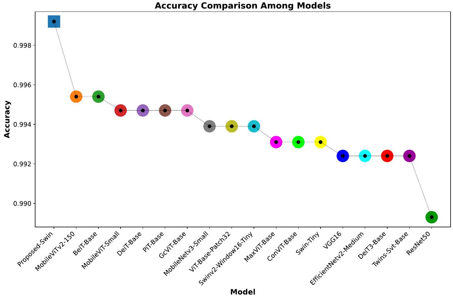
4.5 Results
| Model | Accuracy | Precision | Recall | F1-score |
| VGG16 [67] | 0.9924 | 0.9921 | 0.9917 | 0.9917 |
| ResNet50 [63] | 0.9893 | 0.9887 | 0.9886 | 0.9886 |
| EfficientNetv2-Medium [68] | 0.9924 | 0.9919 | 0.9917 | 0.9917 |
| MobileNetv3-Small [69] | 0.9939 | 0.9936 | 0.9934 | 0.9935 |
| MobileViT-Small [70] | 0.9947 | 0.9942 | 0.9942 | 0.9942 |
| MobileViTv2-150 [71] | 0.9954 | 0.9953 | 0.9950 | 0.9952 |
| MaxViT-Base [72] | 0.9931 | 0.9926 | 0.9927 | 0.9927 |
| DeiT-Base [73] | 0.9947 | 0.9943 | 0.9942 | 0.9942 |
| DeiT3-Base [74] | 0.9924 | 0.9919 | 0.9919 | 0.9919 |
| ViT-Base-Patch32 [57] | 0.9939 | 0.9934 | 0.9934 | 0.9934 |
| BeiT-Base [75] | 0.9954 | 0.9951 | 0.9950 | 0.9950 |
| ConViT-Base [76] | 0.9931 | 0.9928 | 0.9925 | 0.9926 |
| Twins-Svt-Base [77] | 0.9924 | 0.9918 | 0.9924 | 0.9921 |
| PiT-Base [78] | 0.9947 | 0.9943 | 0.9942 | 0.9942 |
| Swin-Tiny [60] | 0.9931 | 0.9927 | 0.9925 | 0.9926 |
| Swinv2-Window16-Tiny [61] | 0.9939 | 0.9935 | 0.9933 | 0.9934 |
| GcViT-Base [79] | 0.9947 | 0.9944 | 0.9942 | 0.9942 |
| Proposed-Swin | 0.9992 | 0.9992 | 0.9992 | 0.9992 |
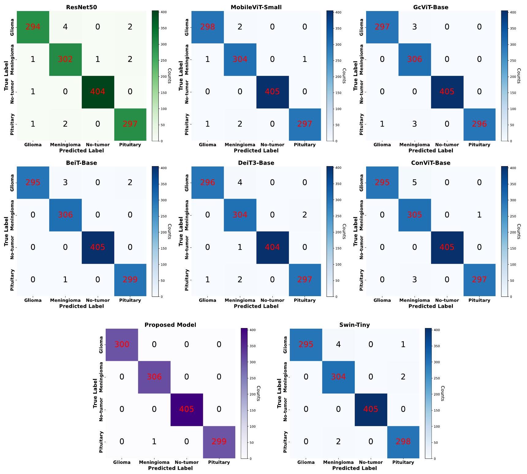
practical implementation in medical imaging and diagnostic systems. Among the models evaluated, the Proposed-Swin model stands out with exceptional results, achieving an outstanding metrics of 0.9992 . This demonstrates the ProposedSwin model is highly effective in accurately classifying brain MRI images, making it a promising candidate for real-world clinical applications.
(Proposed-Swin), followed by MobileViTv2-150, BeiTBase, MobileViT-Small, DeiT-Base, with ResNet50 being the least performing model. Notably, the current model, DeiT3, shows lower performance compared to its predecessor, the DeiT model. This underscores the variability in performance that each model can exhibit on medical datasets.
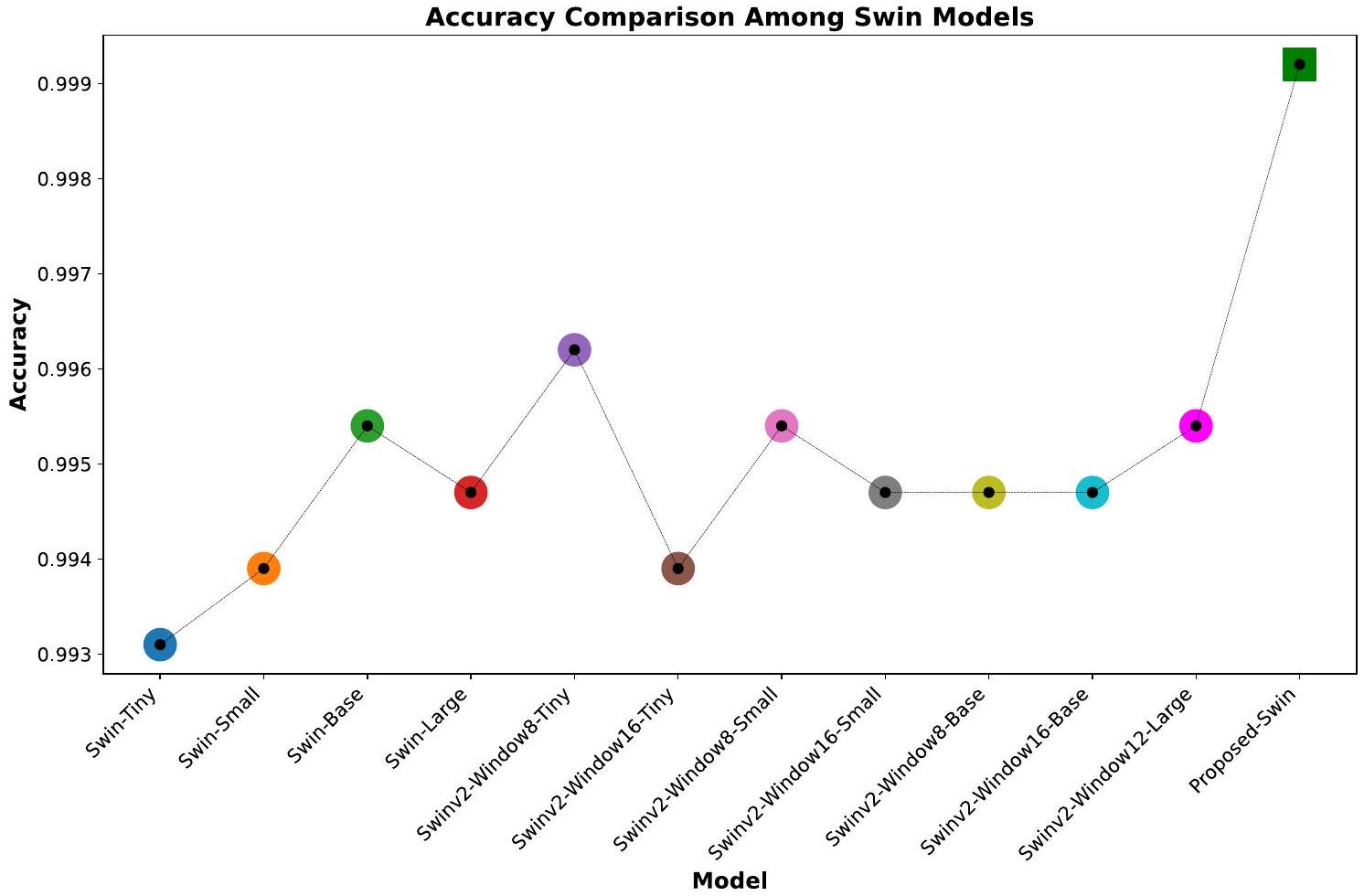
4.6 Efficiency of the proposed-Swin model and Swin transformer variants
of shifted windows. It strategically allocates
4.7 Comparison with cutting-edge methods
| Model | Accuracy | Precision | Recall | F1-score |
| Swin-Tiny | 0.9931 | 0.9927 | 0.9925 | 0.9926 |
| Swin-small | 0.9939 | 0.9935 | 0.9933 | 0.9934 |
| Swin-base | 0.9954 | 0.9951 | 0.9950 | 0.9950 |
| Swin-large | 0.9947 | 0.9944 | 0.9942 | 0.9942 |
| Swinv2-Window8-Tiny | 0.9962 | 0.9961 | 0.9959 | 0.9960 |
| Swinv2-Window16-Tiny | 0.9939 | 0.9935 | 0.9933 | 0.9934 |
| Swinv2-Window8-Small | 0.9954 | 0.9952 | 0.995 | 0.9951 |
| Swinv2-Window16-Small | 0.9947 | 0.9942 | 0.9942 | 0.9942 |
| Swinv2-Window8-Base | 0.9947 | 0.9944 | 0.9942 | 0.9942 |
| Swinv2-Window16-Base | 0.9947 | 0.9943 | 0.9942 | 0.9942 |
| Swinv2-Window12-Large | 0.9954 | 0.9953 | 0.995 | 0.9952 |
| Proposed-Swin | 0.9992 | 0.9992 | 0.9992 | 0.9992 |
classification, particularly focusing on the vital task of diagnosing brain tumors. Amidst the array of methodologies presented by different studies, Proposed-Swin (ViT) stands out as a pinnacle of performance in detecting brain abnormalities. The convergence of advanced computer vision techniques and medical imaging is strikingly evident in the exceptional accuracy of Proposed-Swin (ViT) on Kaggle’s dataset, reaching an impressive
4.8 Limitations and future directions
obtained from various healthcare institutions to enhance the Swin Model’s performance and generalizability. This multi-center validation is crucial for evaluating the model’s performance across different imaging protocols and patient demographics. Additionally, planned studies aim to demonstrate the model’s performance on different medical images. Optimizing the Swin Model for real-time applications is also a significant future direction. Improving the model’s architecture and efficient inference strategies are essential for providing timely and on-site diagnostic support to radiologists.
5 Conclusion
| Author and year | Dataset | Method | Accuracy % |
| Talukder et al., 2023 [13] | Figshare | CNN-based | 99.68 |
| Tabatabaei et al., 2023 [48] | Figshare | CNN + Attention | 99.30 |
| Deepak and Ameer, 2023 [80] | Figshare | CNN+SVM | 95.60 |
| Zulfiqar et al., 2023 [32] | Figshare | CNN-based | 98.86 |
| Ghassemi et al., 2020 [47] | Figshare | CNN+GAN | 95.60 |
| Mehnatkesh et al., 2023 [33] | Figshare | CNN-based | 98.69 |
| Swati et al., 2019 [51] | Figshare | CNN-based | 94.82 |
| Sajjad et al., 2019 [52] | Figshare | CNN-based | 90.67 |
| Rehman et al., 2020 [42] | Figshare | CNN-based | 98.69 |
| Kumar et al., 2021 [41] | Figshare | CNN-based | 97.48 |
| Mzoughi et al., 2020 [44] | BraTS | CNN-based | 96.49 |
| Sharif et al., 2022 [43] | BraTS | CNN-based | 98.80 |
| Ozkaraca et al., 2023 [81] | Kaggle | CNN-based | 96.00 |
| Rahman and Islam, 2023 [82] | Kaggle | CNN-based | 98.12 |
| Muezzinoglu et al., 2023 [83] | Kaggle | CNN-based | 98.10 |
| Ali et al., 2023 [84] | Kaggle | CNN-based | 95.70 |
| Proposed-Swin | Kaggle | Swin-based (ViT) | 99.92 |
Declarations
Ethical approval No ethics approval was required for this work as it did not involve human subjects, animals, or sensitive data that would necessitate ethical review.
References
- Bondy ML, Scheurer ME, Malmer B et al (2008) Brain tumor epidemiology: consensus from the Brain Tumor Epidemiology Consortium. Cancer 113:1953-1968
- Herholz K, Langen KJ, Schiepers C, Mountz JM (2012) Brain tumors. Semin Nucl Med 42:356-370. https://doi.org/10.1053/j. semnuclmed.2012.06.001
- Ostrom QT, Barnholtz-Sloan JS (2011) Current state of our knowledge on brain tumor epidemiology. Curr Neurol Neurosci Rep 11:329-335. https://doi.org/10.1007/s11910-011-0189-8
- Miller KD, Ostrom QT, Kruchko C et al (2021) Brain and other central nervous system tumor statistics, 2021. CA Cancer J Clin 71:381-406. https://doi.org/10.3322/caac. 21693
- Charles NA, Holland EC, Gilbertson R et al (2011) The brain tumor microenvironment. Glia 59:1169-1180. https://doi.org/10. 1002/glia. 21136
- Liu Z, Tong L, Chen L et al (2023) Deep learning based brain tumor segmentation: a survey. Complex Intell Syst 9:1001-1026. https://doi.org/10.1007/s40747-022-00815-5
- Jyothi P, Singh AR (2023) Deep learning models and traditional automated techniques for brain tumor segmentation in MRI: a review. Artif Intell Rev 56:2923-2969. https://doi.org/10.1007/ s10462-022-10245-x
- Solanki S, Singh UP, Chouhan SS, Jain S (2023) Brain tumor detection and classification using intelligence techniques: an overview. IEEE Access 11:12870-12886
- Villanueva-Meyer JE, Mabray MC, Cha S (2017) Current clinical brain tumor imaging. Clin Neurosurg 81:397-415. https://doi.org/ 10.1093/neuros/nyx103
- Ellingson BM, Wen PY, Van Den Bent MJ, Cloughesy TF (2014) Pros and cons of current brain tumor imaging. Neuro Oncol 16:vii2-vii11. https://doi.org/10.1093/neuonc/nou224
- Xie Y, Zaccagna F, Rundo L et al (2022) Convolutional neural network techniques for brain tumor classification (from 2015 to 2022): review, challenges, and future perspectives. Diagnostics 12:1850
- Ali S, Li J, Pei Y et al (2022) A comprehensive survey on brain tumor diagnosis using deep learning and emerging hybrid techniques with multi-modal MR image. Arch Comput Methods Eng 29:4871-4896
- Talukder MA, Islam MM, Uddin MA et al (2023) An efficient deep learning model to categorize brain tumor using reconstruction and fine-tuning. Expert Syst Appl. https://doi.org/10.1016/j. eswa.2023.120534
- Rajeev SK, Pallikonda Rajasekaran M, Vishnuvarthanan G, Arunprasath T (2022) A biologically-inspired hybrid deep learning approach for brain tumor classification from magnetic resonance imaging using improved gabor wavelet transform and Elmann-BiLSTM network. Biomed Signal Process Control. https://doi.org/10.1016/j.bspc.2022.103949
- Pacal I, Kılıcarslan S (2023) Deep learning-based approaches for robust classification of cervical cancer. Neural Comput Appl. https://doi.org/10.1007/s00521-023-08757-w
- Coşkun D, Karaboğa D, Baştürk A et al (2023) A comparative study of YOLO models and a transformer-based YOLOv5 model for mass detection in mammograms. Turk J Electr Eng Comput Sci 31:1294-1313. https://doi.org/10.55730/13000632.4048
- Wang W, Pei Y, Wang SH et al (2023) PSTCNN: explainable COVID-19 diagnosis using PSO-guided self-tuning CNN. Biocell 47:373-384. https://doi.org/10.32604/biocell.2023.025905
- Pacal I, Karaboga D (2021) A robust real-time deep learning based automatic polyp detection system. Comput Biol Med. https://doi. org/10.1016/j.compbiomed.2021.104519
- Zhang Y-D, Govindaraj VV, Tang C et al (2019) High performance multiple sclerosis classification by data augmentation and AlexNet transfer learning model. J Med Imaging Health Inform 9:2012-2021. https://doi.org/10.1166/JMIHI.2019.2692
- Wang W, Zhang X, Wang SH, Zhang YD (2022) COVID-19 diagnosis by WE-SAJ. Syst Sci Control Eng 10:325-335. https://doi. org/10.1080/21642583.2022.2045645
- Pacal I (2022) Deep learning approaches for classification of breast cancer in ultrasound (US) images. J Inst Sci Technol. https://doi.org/10.21597/jist. 1183679
- Amin J, Sharif M, Haldorai A et al (2022) Brain tumor detection and classification using machine learning: a comprehensive survey. Complex Intell Syst 8:3161-3183. https://doi.org/10.1007/ s40747-021-00563-y
- Deepak S, Ameer PM (2019) Brain tumor classification using deep CNN features via transfer learning. Comput Biol Med. https://doi.org/10.1016/j.compbiomed.2019.103345
- Wang SH, Govindaraj VV, Górriz JM et al (2021) Covid-19 classification by FGCNet with deep feature fusion from graph convolutional network and convolutional neural network. Inform Fusion 67:208-229. https://doi.org/10.1016/j.inffus.2020.10.004
- Chahal PK, Pandey S, Goel S (2020) A survey on brain tumor detection techniques for MR images. Multimed Tools Appl 79:21771-21814. https://doi.org/10.1007/s11042-020-08898-3
- Amin J, Sharif M, Yasmin M, Fernandes SL (2018) Big data analysis for brain tumor detection: deep convolutional neural networks. Futur Gener Comput Syst 87:290-297. https://doi.org/10. 1016/j.future.2018.04.065
- Esmaeili M, Vettukattil R, Banitalebi H et al (2021) Explainable artificial intelligence for human-machine interaction in brain tumor localization. J Pers Med. https://doi.org/10.3390/jpm11 111213
- Zhang Y, Deng L, Zhu H et al (2023) Deep learning in food category recognition. Inform Fusion. https://doi.org/10.1016/j.inffus. 2023.101859
- Karaman A, Karaboga D, Pacal I et al (2022) Hyper-parameter optimization of deep learning architectures using artificial bee colony (ABC) algorithm for high performance real-time automatic colorectal cancer (CRC) polyp detection. Appl Intell. https://doi. org/10.1007/s10489-022-04299-1
- Pacal I, Karaman A, Karaboga D et al (2022) An efficient realtime colonic polyp detection with YOLO algorithms trained by using negative samples and large datasets. Comput Biol Med. https://doi.org/10.1016/J.COMPBIOMED.2021.105031
- Pacal I, Alaftekin M (2023) Türk İşaret Dilinin Sınıflandırılması için Derin Öğrenme Yaklaşımları. Iğdır Üniversitesi Fen Bilimleri Enstitüsü Dergisi 13:760-777. https://doi.org/10.21597/jist. 12234 57
- Zulfiqar F, Ijaz Bajwa U, Mehmood Y (2023) Multi-class classification of brain tumor types from MR images using EfficientNets. Biomed Signal Process Control. https://doi.org/10.1016/j.bspc. 2023.104777
- Mehnatkesh H, Jalali SMJ, Khosravi A, Nahavandi S (2023) An intelligent driven deep residual learning framework for brain tumor classification using MRI images. Expert Syst Appl. https:// doi.org/10.1016/j.eswa.2022.119087
- Shamshad F, Khan S, Zamir SW et al (2023) Transformers in medical imaging: a survey. Med Image Anal 88:102802
- Akinyelu AA, Zaccagna F, Grist JT et al (2022) Brain tumor diagnosis using machine learning, convolutional neural networks, capsule neural networks and vision transformers, applied to MRI: a survey. J Imaging 8:205
- Celard P, Iglesias EL, Sorribes-Fdez JM et al (2023) A survey on deep learning applied to medical images: from simple artificial neural networks to generative models. Neural Comput Appl 35:2291-2323
- Tummala S, Kadry S, Bukhari SAC, Rauf HT (2022) Classification of brain tumor from magnetic resonance imaging using vision transformers ensembling. Curr Oncol 29:7498-7511. https://doi. org/10.3390/curroncol29100590
- Karaman A, Pacal I, Basturk A et al (2023) Robust real-time polyp detection system design based on YOLO algorithms by optimizing activation functions and hyper-parameters with artificial bee colony (ABC). Expert Syst Appl. https://doi.org/10.1016/j.eswa. 2023.119741
- Nazir M, Shakil S, Khurshid K (2021) Role of deep learning in brain tumor detection and classification (2015 to 2020): a review. Comput Med Imaging Graph. https://doi.org/10.1016/j.compm edimag.2021.101940
- Jiang Y, Zhang Y, Lin X et al (2022) SwinBTS: a method for 3D multimodal brain tumor segmentation using Swin transformer. Brain Sci. https://doi.org/10.3390/brainsci12060797
- Kumar RL, Kakarla J, Isunuri BV, Singh M (2021) Multi-class brain tumor classification using residual network and global average pooling. Multimed Tools Appl 80:13429-13438. https://doi. org/10.1007/s11042-020-10335-4
- Rehman A, Naz S, Razzak MI et al (2020) A deep learning-based framework for automatic brain tumors classification using transfer learning. Circuits Syst Signal Process 39:757-775. https://doi.org/ 10.1007/s00034-019-01246-3
- Sharif MI, Khan MA, Alhussein M et al (2022) A decision support system for multimodal brain tumor classification using deep learning. Complex Intell Syst 8:3007-3020. https://doi.org/10. 1007/s40747-021-00321-0
- Mzoughi H, Njeh I, Wali A et al (2020) Deep multi-scale 3D convolutional neural network (CNN) for MRI gliomas brain tumor classification. J Digit Imaging 33:903-915. https://doi.org/10. 1007/s10278-020-00347-9
- Amin J, Sharif M, Raza M et al (2019) Brain tumor detection using statistical and machine learning method. Comput Methods Programs Biomed 177:69-79. https://doi.org/10.1016/j.cmpb. 2019.05.015
- Tandel GS, Balestrieri A, Jujaray T et al (2020) Multiclass magnetic resonance imaging brain tumor classification using artificial intelligence paradigm. Comput Biol Med. https://doi.org/10. 1016/j.compbiomed.2020.103804
- Ghassemi N, Shoeibi A, Rouhani M (2020) Deep neural network with generative adversarial networks pre-training for brain tumor classification based on MR images. Biomed Signal Process Control. https://doi.org/10.1016/j.bspc.2019.101678
- Tabatabaei S, Rezaee K, Zhu M (2023) Attention transformer mechanism and fusion-based deep learning architecture for MRI brain tumor classification system. Biomed Signal Process Control. https://doi.org/10.1016/j.bspc.2023.105119
- Kumar S, Mankame DP (2020) Optimization driven deep convolution neural network for brain tumor classification. Biocybern Biomed Eng 40:1190-1204. https://doi.org/10.1016/j.bbe.2020.05.009
- Amin J, Sharif M, Yasmin M, Fernandes SL (2020) A distinctive approach in brain tumor detection and classification using MRI. Pattern Recognit Lett 139:118-127. https://doi.org/10.1016/j. patrec.2017.10.036
- Swati ZNK, Zhao Q, Kabir M et al (2019) Brain tumor classification for MR images using transfer learning and fine-tuning. Comput Med Imaging Graph 75:34-46. https://doi.org/10.1016/j. compmedimag.2019.05.001
- Sajjad M, Khan S, Muhammad K et al (2019) Multi-grade brain tumor classification using deep CNN with extensive data augmentation. J Comput Sci 30:174-182. https://doi.org/10.1016/j.jocs.2018.12.003
- Brain tumor dataset. https://figshare.com/articles/dataset/brain_ tumor_dataset/1512427. Accessed 30 Jul 2023
- Brain Tumor Classification (MRI) I Kaggle. https://www.kag-gle.com/datasets/sartajbhuvaji/brain-tumor-classification-mri. Accessed 30 Jul 2023
- Br35H :: Brain Tumor Detection 2020 | Kaggle. https://www.kag-gle.com/datasets/ahmedhamada0/brain-tumor-detection?select= no. Accessed 30 Jul 2023
- Brain Tumor MRI Dataset I Kaggle. https://www.kaggle.com/ datasets/masoudnickparvar/brain-tumor-mri-dataset?select=Train ing. Accessed 30 Jul 2023
- Dosovitskiy A, Beyer L, Kolesnikov A et al (2020) An image is Worth
words: transformers for image recognition at scale. In: ICLR 2021-9th International Conference on Learning Representations - Pacal I (2024) Enhancing crop productivity and sustainability through disease identification in maize leaves: exploiting a large dataset with an advanced vision transformer model. Expert Syst Appl. https://doi.org/10.1016/j.eswa.2023.122099
- Khan S, Naseer M, Hayat M et al (2021) Transformers in vision: a survey. ACM Comput Surv. https://doi.org/10.1145/3505244
- Liu Z, Lin Y, Cao Y, et al (2021) Swin transformer: hierarchical vision transformer using shifted windows
- Liu Z, Hu H, Lin Y, et al (2021) Swin transformer V2: scaling up capacity and resolution
- Touvron H, Bojanowski P, Caron M, et al (2021) ResMLP: feedforward networks for image classification with data-efficient training
- He K, Zhang X, Ren S, Sun J (2016) Deep residual learning for image recognition. In: Proceedings of the IEEE Computer Society Conference on Computer Vision and Pattern Recognition 2016Decem, pp 770-778. https://doi.org/10.1109/CVPR.2016.90
- Russakovsky O, Deng J, Su H et al (2015) ImageNet large scale visual recognition challenge. Int J Comput Vis 115:211-252. https://doi.org/10.1007/s11263-015-0816-y
- Krizhevsky A, Sutskever I, Hinton GE (2017) ImageNet classification with deep convolutional neural networks. Commun ACM 60:84-90. https://doi.org/10.1145/3065386
- Krizhevsky A, Sutskever I, Hinton GE (2012) ImageNet classification with deep convolutional neural networks. In: Pereira F, Burges CJ, Bottou L, Weinberger KQ (eds) Advances in neural information processing systems. Curran Associates Inc
- Simonyan K, Zisserman A (2015) Very deep convolutional networks for large-scale image recognition. In: 3rd International Conference on Learning Representations, ICLR 2015-Conference Track Proceedings, pp 1-14
- Tan M, Le Q V (2021) EfficientNetV2: smaller models and faster training
- Howard A, Sandler M, Chen B, et al (2019) Searching for mobileNetV3. In: Proceedings of the IEEE International Conference on Computer Vision. Institute of Electrical and Electronics Engineers Inc., pp 1314-1324
- Mehta S, Rastegari M (2021) MobileViT: light-weight, generalpurpose, and mobile-friendly vision transformer. 3
- Mehta S, Rastegari M (2022) Separable self-attention for mobile vision transformers
- Tu Z, Talebi H, Zhang H, et al (2022) MaxViT: multi-axis vision transformer. Lecture Notes in computer science (including subseries lecture notes in artificial intelligence and lecture notes in bioinformatics) 13684 LNCS, pp 459-479. https://doi.org/10. 1007/978-3-031-20053-3_27
- Touvron H, Cord M, Douze M, et al (2020) Training data-efficient image transformers & distillation through attention, pp 1-22
- Touvron H, Cord M, Ai M DeiT III : Revenge of the ViT. 1-27
- Bao H, Dong L, Piao S, Wei F (2021) BEiT: BERT pre-training of image transformers
- d’Ascoli S, Touvron H, Leavitt M, et al (2021) ConViT: improving vision transformers with soft convolutional inductive biases. https://doi.org/10.1088/1742-5468/ac9830
- Chu X, Tian Z, Wang Y et al (2021) Twins: revisiting the design of spatial attention in vision transformers. Adv Neural Inf Process Syst 12:9355-9366
- Heo B, Yun S, Han D, et al (2021) Rethinking spatial dimensions of vision transformers
- Hatamizadeh A, Yin H, Heinrich G, et al (2022) Global context vision transformers
- Deepak S, Ameer PM (2023) Brain tumor categorization from imbalanced MRI dataset using weighted loss and deep feature fusion. Neurocomputing 520:94-102. https://doi.org/10.1016/j. neucom.2022.11.039
- Ozkaraca O, Bağrıaçık Oİ, Gürüler H et al (2023) Multiple brain tumor classification with dense CNN architecture using brain MRI images. Life. https://doi.org/10.3390/life13020349
- Rahman T, Islam MS (2023) MRI brain tumor detection and classification using parallel deep convolutional neural networks. Meas Sens. https://doi.org/10.1016/j.measen.2023.100694
- Muezzinoglu T, Baygin N, Tuncer I et al (2023) PatchResNet: Multiple patch division-based deep feature fusion framework for brain tumor classification using MRI images. J Digit Imaging 36:973-987. https://doi.org/10.1007/s10278-023-00789-x
- Ali MU, Hussain SJ, Zafar A et al (2023) WBM-DLNets: wrapperbased metaheuristic deep learning networks feature optimization for enhancing brain tumor detection. Bioengineering. https://doi. org/10.3390/bioengineering10040475
- Ishak Pacal
ishak.pacal@igdir.edu.tr
1 Department of Computer Engineering, Faculty of Engineering, Igdir University, 76000 Igdir, Turkey