هيكل جديد لشبكة عصبية تلافيفية للكشف المبكر الدقيق وتصنيف مرض الزهايمر باستخدام بيانات الرنين المغناطيسي A novel CNN architecture for accurate early detection and classification of Alzheimer’s disease using MRI data
هيكل جديد لشبكة عصبية تلافيفية للكشف المبكر الدقيق وتصنيف مرض الزهايمر باستخدام بيانات الرنين المغناطيسي
أ. م. العاصيحنان م. عامرح. م. إبراهيموم. أ. محمد
الملخص
مرض الزهايمر (AD) هو اضطراب عصبي تنكسي مُعطِّل يتطلب تشخيصًا دقيقًا لإدارة فعالة وعلاج. في هذه المقالة، نقترح هيكلًا لشبكة عصبية تلافيفية (CNN) تستخدم بيانات التصوير بالرنين المغناطيسي (MRI) من مجموعة بيانات مبادرة تصوير مرض الزهايمر (ADNI) لتصنيف مرض الزهايمر. تستخدم الشبكة نموذجين منفصلين من CNN، كل منهما بحجم مرشح مختلف وطبقات تجميع، والتي يتم دمجها في طبقة التصنيف. يتم معالجة المشكلة متعددة الفئات عبر ثلاث، أربع، وخمس فئات. تحقق بنية CNN المقترحة دقة استثنائية من، ، و ، على التوالي. تُظهر هذه الدقة العالية فعالية الشبكة في التقاط وتمييز الميزات ذات الصلة من صور الرنين المغناطيسي، مما يمكّن من تصنيف دقيق لأنواع وأطوار مرض الزهايمر. تستفيد بنية الشبكة من الطبيعة الهرمية للطبقات التلافيفية، وطبقات التجميع، وطبقات الاتصال الكامل لاستخراج الأنماط المحلية والعالمية من البيانات، مما يسهل التمييز الدقيق بين فئات مرض الزهايمر المختلفة. يحمل التصنيف الدقيق لمرض الزهايمر تداعيات سريرية هامة، بما في ذلك الكشف المبكر، وتخطيط العلاج الشخصي، ومراقبة المرض، وتقييم التنبؤ. تؤكد الدقة المبلغ عنها على إمكانيات بنية الشبكة العصبية المقترحة لمساعدة المتخصصين الطبيين والباحثين في اتخاذ أحكام دقيقة ومستنيرة بشأن مرضى الزهايمر.
الكلمات الرئيسية: مرض الزهايمر، الشبكة العصبية التلافيفية، التعلم العميق، الأنظمة الذكية، قابلية التفسير
مرض في الدماغ يسمى مرض الزهايمر (AD) أصبح شائعًا بشكل متزايد مع مرور الوقت ويحتل الآن المرتبة الرابعة كأحد الأسباب الرئيسية للوفاة في الدول الصناعية. فقدان الذاكرة وضعف الإدراك يمثلان أكثر العلامات شيوعًا للزهايمر، الناتجة عن موت وتدمير خلايا الأعصاب المرتبطة بالذاكرة في الدماغ.بين الوظيفة الطبيعية للدماغ ومرض الزهايمر توجد حالة تُعرف باسم ضعف الإدراك الخفيف.. تدريجياً، من المرحلة البادئة لضعف الإدراك المعتدل، يتقدم مرض الزهايمر إلى الخرف. تشير الدراسات إلى أن مرض الزهايمر يتطور لدى المرضى الذين يعانون من ضعف الإدراك المعتدل بمعدل في السنةيمكن أن يؤدي التعرف المبكر على مرضى ضعف الإدراك المعتدل إلى إيقاف أو تأخير التقدم من مرحلة ضعف الإدراك المعتدل إلى مرض الزهايمر. يظهر المرضى في المراحل المتوسطة من ضعف الإدراك المعتدل اختلافات شكلية دقيقة في آفات دماغهم..
تُبرز الدراسات الحديثة أن ضعف الإدراك المعرفي الخفيف المبكر (EMCI) يظهر في المراحل الأولية من ضعف الإدراك المعرفي. في المقابل، يشير ضعف الإدراك المعرفي الخفيف المتأخر (LMCI) أو ضعف الإدراك المعرفي الخفيف التقدمي (PMCI) إلى أعراض تتدهور مع مرور الوقت.مع تقدم الأعراض وانتقالها بين المراحل، يمارس المتخصصون في الرعاية الصحية مزيدًا من الحذر.يمكن أن يشكل تحديد التباينات في الأعراض المحددة عبر مجموعات مختلفة تحديات للباحثين. تشمل تقنيات التصوير الطبي المختلفة، مثل تصوير الانبعاثات البوزيترونية (PET)التصوير بالرنين المغناطيسي (MRI) والتصوير المقطعي المحوسب (CT)تقدم تنسيقات اختبار قياسية وصورًا أساسية لعمليات التجريب لهذه الأنماط.
تتميز الرنين المغناطيسي كأداة فعالة وآمنة، ومعترف بها على نطاق واسع لتشخيص مجموعة من الأمراض بما في ذلك أورام الدماغ.اضطرابات عصبيةإصابات الحبل الشوكي والعيوبوأمراض الكبد. تُعزى هذه المرونة إلى حساسيتها العالية، مما يسهل الكشف المبكر عن الأمراض. تمتلك تسلسلات التصوير بالرنين المغناطيسي قدرات فريدة تناسب اضطرابات مختلفة. بالمقارنة مع تقنيات التصوير الأخرى، فإن صور الرنين المغناطيسي هي
يتم استخدامه بشكل متكرر لتصنيف مرض الزهايمر. ومع ذلك، فإن الميزات المختلفة المستخرجة من صور الرنين المغناطيسي تساعد في تصنيف وتشخيص ضعف الإدراك المعتدل أو مرض الزهايمر، بما في ذلك أحجام المادة الرمادية والبيضاء، وسمك القشرة، ومستويات السائل الدماغي الشوكي، مما يساعد في تحديد مرحلة المرض.لقد أظهرت الشبكات العصبية التلافيفية المدربة مسبقًا مؤخرًا وعدًا في تشخيص الأمراض المعرفية تلقائيًا من صور الرنين المغناطيسي للدماغ. تشمل الشبكات العصبية العميقة الملحوظة التي تم تدريبها مسبقًا وتطبيقها على بيانات الرنين المغناطيسي شبكة أليكس-نت.VGG16ريزنت-18ريزنت-34ResNet-50¹8، بالإضافة إلى Squeeze-Net و InceptionV3.
عادةً ما يتم تحسين الشبكات العميقة الموجودةقد لا تعالج دائمًا الكفاءة المنخفضة في النقل الناتجة عن الفجوات بين الصور الطبية وغير الطبية. علاوة على ذلك، يمكن أن تساهم العديد من العوامل في الإفراط في التكيف والاستخدام غير الفعال للمساحة. لتمييز بين المرضى الذين يعانون من مرض الزهايمر (AD)، والمرحلة المبكرة من مرض الزهايمر (EMCI)، والاضطراب المعرفي المعتدل (MCI)، والمرحلة المتأخرة من الاضطراب المعرفي المعتدل (LMCI)، وأولئك الذين يتمتعون بقدرات معرفية طبيعية (CN)، نقترح نهجًا مبتكرًا لتطوير نماذج الشبكات العصبية التلافيفية (CNN)، لتحقيق دقة عالية في مهام التصنيف المتعدد الفئات، خاصة في تصنيف صور الرنين المغناطيسي.
تشمل المساهمات الرئيسية لورقتنا:
نموذج هيكل CNN الجديد: نقدم نموذجين مبسطين من CNN، كل منهما يمتلك هيكلاً بسيطاً. على الرغم من بساطتهما، تحقق هذه النماذج تقريباًالدقة في مشكلة التصنيف ذات الخمس فئات، مما يوضح أنه يمكن تصميم نماذج فعالة دون تعقيد مفرط.
أثر حجم الفلتر: تُظهر دراستنا أن تقليل حجم الفلتر يمكن أن يؤدي إلى تحسين نتائج التصنيف. على سبيل المثال، يستخدم CNN2 حجم الفلتر، يتطلب ضعف عدد الفلاتر في CNN1، معحجم الفلتر، لتحقيق مستويات دقة مماثلة.
تقنية الربط: نقدم نهجًا جديدًا من خلال دمج نموذجين متطورين من الشبكات العصبية التلافيفية في طبقة التصنيف، مبتعدين عن الطرق السابقة التي تدمج النماذج المدربة مسبقًا.. نهجنا في الربط يعزز الدقة من 95 إلىفي مهمة التصنيف ذات الخمس طرق، تقدم فوائد مزدوجة: تمكين النماذج من تعلم ميزات محددة للمهمة وتكملة قدرات بعضها البعض.
أداء التصنيف متعدد الفئات: نقوم بتوسيع منهجيتنا لمعالجة تحديات التصنيف متعدد الفئات، وهو انحراف عن العديد من الدراسات التي تركز على الفئات الثنائية أو الفئات الفردية ضمن مشاكل التصنيف متعدد الفئات. باستخدام بيانات MRI من ADNI، نطبق نهجنا على مهام التصنيف ثلاثي الاتجاهات، وأربعة اتجاهات، وخمسة اتجاهات، محققين معدلات دقة ممتازة من، و على التوالي، مما يبرز قابلية التكيف والموثوقية لاستراتيجيتنا عبر سيناريوهات التصنيف المتنوعة.
تحليل مقارن: من خلال الاستفادة من بيانات التصوير بالرنين المغناطيسي، يقوم بحثنا بإجراء تحليل مقارن شامل بين طريقتنا المقترحة والتقنيات السائدة في الكشف عن مرض الزهايمر. توضح هذه الدراسة تفوق أو تقدم نهجنا على الطرق السابقة، مع تقييمه بناءً على مقاييس الدقة.
الأقسام التالية منظمة على النحو التالي: القسم “الأعمال ذات الصلة” يقدم أحدث الدراسات حول الكشف المبكر عن مرض الزهايمر. القسم “المواد” يحدد مجموعة البيانات المستخدمة في بحثنا ومنهجية إعدادها. القسم “وصف نموذج CNN المقترح” يوضح نموذجنا الموصى به لتشخيص مرض الزهايمر. القسم “المناقشة” يكشف عن النتائج التجريبية على مجموعة بيانات ADNI، مصحوبة بمناقشات شاملة ومقارنات مع الأبحاث السابقة. أخيرًا، القسم “الاستنتاج” يلخص استنتاجاتنا.
الأعمال ذات الصلة
في السنوات الأخيرة، كان هناك زيادة في تطبيق تقنيات التعلم العميق لتصنيف مرض الزهايمر (AD) باستخدام بيانات من تصوير الدماغ متعدد الأنماط. من خلال الاستفادة من البيانات الغنية التي توفرها العديد من أنماط التصوير، اقترحت عدة دراسات بحثية شبكات عصبية تلافيفية عميقة محسّنة (CNNs) لتصنيف مرض الزهايمر.
لتوقع تحويل MCI، مؤلفو طوروا نموذجًا يعتمد على التعلم لنقل المجال. استخدموا أنماطًا مختلفة، مستفيدين من عينات بيانات المجال المستهدف والمساعد. بعد اتباع الإجراءات التجريبية، استخدموا التعلم لنقل المجال، محققين دقة توقعات تبلغمرجعقدمت منهجية قوية للتعلم العميق باستخدام تقنيات التصوير بالرنين المغناطيسي وPET. وقد دمجوا استراتيجية الانسحاب لتعزيز الأداء من حيث التصنيف. بالإضافة إلى ذلك، طبقوا طريقة التعلم المتعدد المهام في إطار التعلم العميق، مع تقييم التغيرات مع وبدون انسحاب. وقد أسفرت تقنية الانسحاب عن نتائج تجريبية تشير إلى تحسين.قدم المؤلفون نموذجين قائمين على الشبكات العصبية التلافيفية، حيث قاموا بتقييم الشبكات العصبية التلافيفية الحجمية والمتعددة الرؤى في اختبارات التصنيف ودمجوا تصفية متعددة الدقة، مما أثر بشكل مباشر على نتائج التصنيف.
مؤلفواقترح طريقة CNN ثنائية الأبعاد تعتمد على ResNet50، تتضمن عدة تقنيات لتطبيع الدفعات وخوارزميات تنشيط لتصنيف شرائح الدماغ إلى ثلاث فئات: NC، MCI، وAD. حقق النموذج المقترح معدل دقة قدرهلتحديد سمات شكلية محلية محددة في الدماغ ضرورية لتشخيص مرض الزهايمر، أجريت دراسة أخرىطوروا نهج تعلم عميق يعتمد على SegNet، ووجدوا أن استخدام تقنية التعلم العميق ونموذج مدرب مسبقًا عزز بشكل كبير أداء المصنف.تم تصميم شبكة عصبية تلافيفية ثلاثية الأبعاد للتمييز بين مرض الزهايمر والحالة الطبيعية باستخدام صور الرنين المغناطيسي الوظيفي في حالة الراحة. في الوقت نفسه، قام جيلبي وآخرون.استخدمت صور المورفومترية من معالجة بيانات التصوير بالرنين المغناطيسي (MRI) باستخدام المورفومترية المعتمدة على التنسور (TBM). استخدمت دراستهم طريقة التعلم العميق المعتمدة على بنية Xception القائمة على الكتل الكثيفة، محققة دقة عالية في تشخيص مرض الزهايمر في مراحله المبكرة. ومع ذلك، لم تتناول هذه الدراسة قضايا مثل تباين مجموعة البيانات، والتكيف الزائد، والتحديات المتعلقة باستخراج ميزات صور TBM.
لتشخيص مرض الزهايمر، باجلات وآخرون.اقترح نماذج هجينة تعتمد على التعلم الآلي باستخدام SVM، وغابة عشوائية، والانحدار اللوجستي. استخدمت نماذجهم مسحات مرضى التصوير بالرنين المغناطيسي من مجموعة بيانات OASIS. سلاهي وآخرون. التحليل أكد أن استخدام نهج التعلم العميق سيعزز من توقعات مرض الزهايمر في مراحله المبكرة. لقد استخدموا مجموعات بيانات OASIS و ADNI، على التوالي. فؤادة وآخرون.قدمت نموذج تصنيف يعتمد على شبكة عصبية تلافيفية (CNN) مستندة إلى AlexNet، محققة دقة تصل إلى 95% باستخدام مجموعة من صور الرنين المغناطيسي المتعلقة بمرض الزهايمر.
مورغان وآخرونقدموا نموذج CNN للتعرف على مرض الزهايمر. يتكون النموذج المقترح من طبقتين تلافيفيتين، وطبقة تجميع قصوى، وأربعة كتل شبكة خرف، محققًا دقة قدرهاباستخدام مجموعة بيانات صور الرنين المغناطيسي ADNI. استخدم سلاهي وآخرون، في دراسة أخرى، صور الرنين المغناطيسي لتشخيص مرض الزهايمر باستخدام شبكة عصبية تلافيفية، محققين دقة متوسطة قدرها. في الوقت نفسه، نو وآخرون.اقترح نموذج 3D-CNN-LSTM، مستخدمًا مستخلصات للميزات المكانية والزمانية وحقق نتائج دقة عالية من، و .
رالا باندي وآخرونقدموا نظامًا للتشخيص المبكر وتصنيف مرض الزهايمر (AD) والخلل المعرفي المعتدل (MCI) لدى الأفراد المسنين الذين يتمتعون بقدرات معرفية طبيعية، باستخدام قاعدة بيانات ADNI. حقق نموذجهم الدقة عبر تقنيات التعلم الآلي المختلفة. علاوة على ذلك، أودوسامي وآخرون.قدم نموذج هجين من شبكة عصبية تلافيفية مدربة مسبقًا، يستخدم دمج الميزات العميقة، وت randomization الوزن، ورسم خرائط تنشيط الفئة المعتمدة على التدرج لتعزيز تحديد مرض الزهايمر. بامبر وآخرون.طور شبكة عصبية تلافيفية باستخدام طبقة تلافيفية ضحلة لتصنيف مرض الزهايمر في قطع الصور الطبية، محققًا دقة قدرها. بالإضافة إلى ذلك، نموذج AlzheimerNet الخاص بـ Akter وآخرون، وهو نموذج معدل من InceptionV3أظهر دقة استثنائية في تصنيف مراحل مرض الزهايمر من صور الرنين المغناطيسي للدماغ، متجاوزًا الطرق التقليدية بدقة اختبار تبلغ.
المواد
توضح هذه القسم مصدر البيانات المستخدم لتدريب نموذج CNN للتعرف على مراحل مرض الزهايمر وطرق معالجة الصور المطبقة على مجموعة البيانات.
وصف مجموعة بيانات AD
على الإنترنت، يمكن استخدام العديد من مجموعات البيانات لتصنيف مرض الزهايمر. ومع ذلك، فإن بعض مجموعات بيانات مرض الزهايمر بتنسيق CSV غير مناسبة لهذه الدراسة. الوصول إلى مجموعات البيانات من منظمات مخصصة مثل كاجل،وأوآسيسمتاح لأغراض البحث والتعليم. تحتوي مجموعة بيانات MRI ADNI على صور الرنين المغناطيسي المستخدمة في هذه الدراسة. تشمل مجموعة بيانات مبادرة تصوير مرض الزهايمر (ADNI) مرضى مصابين بمرض الزهايمر، وضعف إدراكي خفيف (MCI)، وأشخاص أصحاء. تشمل مجموعة بيانات ADNI معلومات جينية، اختبارات معرفية، مؤشرات حيوية في الدم والسائل الدماغي الشوكي، صور الرنين المغناطيسي وPET، بالإضافة إلى معلومات سريرية. تقدم الجدول 1 معلومات إحصائية تتعلق بمجموعة بيانات MRI ADNI.
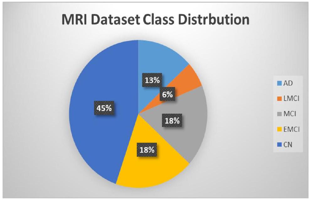
تتكون هذه البيانات من 1296 صورة رنين مغناطيسي بتقنية T1. كل صورة تنتج صورة ثلاثية الأبعاد للدماغ بدقة 1.5 مم من الفوكسيلا المتساوية. كما هو موضح في الشكل 1، يتم تصنيف الصور إلى واحدة من خمس فئات: مرضى CN، EMCI، LMCI، AD، وMCI.
الشكل 1. توزيع الفئات لمجموعة بيانات الرنين المغناطيسي.
معالجة البيانات المسبقة
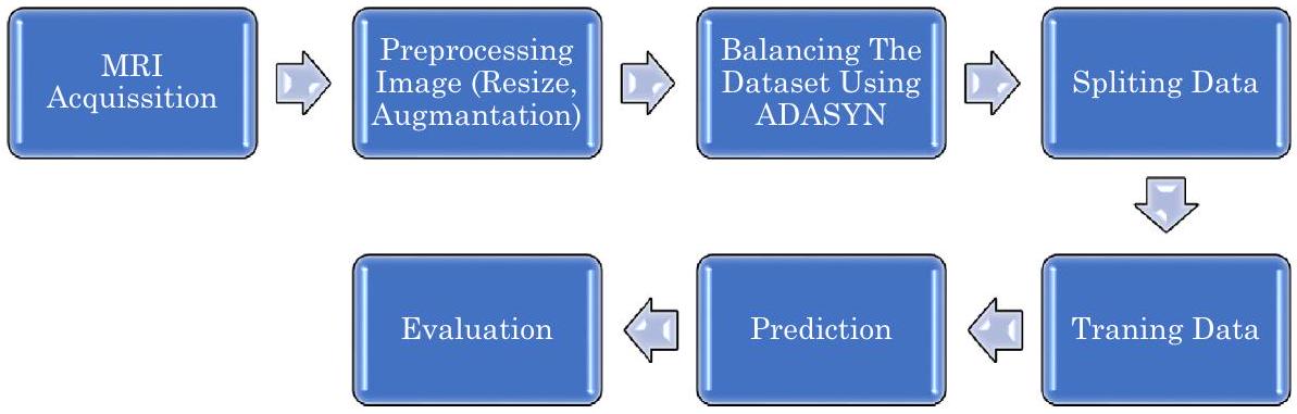
تم اختيار مجموعة بيانات ADNI لهذه الدراسة بناءً على ملاءمتها لأهداف بحثنا. تمثل مجموعة بيانات ADNI، التي ساهمت بها مبادرة تصوير الأعصاب لمرض الزهايمر (ADNI)، جهدًا بحثيًا عالميًا يهدف إلى تطوير والتحقق من أدوات تصوير الأعصاب لتتبع تقدم مرض الزهايمر (AD). تتكون هذه المجموعة من بيانات تم جمعها من مراكز تصوير ADNI، الموجودة في العيادات والمؤسسات الطبية في جميع أنحاء الولايات المتحدة وأجزاء أخرى من العالم. قبل إصدارها للجمهور، خضعت البيانات لعمليات معالجة وتحضير من قبل مختبرات تحليل التصوير بالرنين المغناطيسي الممولة من ADNI. لتحسين جودة وتناسق الصور للتحليل، خضعت صور مجموعة البيانات لخطوات معالجة مسبقة أساسية. كما هو موضح في الشكل 2، شملت هذه الخطوات:
التكبير: تغيير حجم جميع الصور بشكل موحد إلى 224 بكسل في كل من العرض والارتفاع.
التعزيز: تعزيز تنوع مجموعة البيانات والتقليل من الإفراط في التكيف من خلال استخدام تقنيات تعزيز البيانات، كما هو مذكور في.
لمعالجة مشكلة عدم توازن الفئات داخل مجموعة البيانات، كما هو موضح في الشكل 1، استخدمنا تقنية ADASYN لتوليد بيانات اصطناعية للفئات الممثلة تمثيلاً ناقصاً.
زيادة البيانات
لتقليل الإفراط في التكيف أثناء تدريب الشبكات العصبية، يتم استخدام تحسين البيانات. تتضمن هذه التقنية إجراء تغييرات تحافظ على الفئة على البيانات الفردية، مما يؤدي إلى توسيع مجموعة البيانات بشكل مصطنع.استخدام طرق تضمن إمكانية التكرار يسمح بإنشاء عينات جديدة دون تغيير المعنى الدلالي للصورة. نظرًا للتحديات المتعلقة بالعثور يدويًا على الصور الموصوفة حديثًا في المجال الطبي وتوافر المعرفة المتخصصة المحدود، تظهر زيادة البيانات كطريقة موثوقة لتوسيع مجموعة البيانات.
لعملنا، وضعنا طريقة لتكبير الصور تتضمن القص، والتكبير، والانعكاس، وضبط السطوع والتباين في الصور.
تقنية ADASYN لموازنة مجموعة بيانات AD
هناك طريقتان قياسيتان قياسيتان: الزيادة في العينة وتقليل العينة. الزيادة في العينة تخلق عينات لفئة الأقلية، بينما تقليل العينة يقلل من العينات من فئة الأغلبية. في الاستراتيجية المقترحة، نستخدم تقنية زيادة العينة المسماة ADASYN.ADASYN تعني نهج العينة الاصطناعية التكيفية، وهي تقنية في تعلم الآلة مصممة لمعالجة عدم التوازن في مجموعات البيانات. مثل SMOTE (تقنية زيادة العينة الاصطناعية للأقليات)، تهدف ADASYN إلى تحسين أداء نماذج التصنيف من خلال زيادة عدد النقاط البيانية في الفئة الأقل تمثيلاً بشكل اصطناعي. ومع ذلك، تستخدم ADASYN نهجًا أكثر تعقيدًا من SMOTE.
المفهوم الأساسي لـ ADASYN يتضمن استخدام توزيعات موزونة لمختلف أمثلة الفئة الأقل بناءً على الصعوبة التي يواجهها المتعلم في فهمها. هذا يخلق بيانات أكثر شمولاً للحالات الأكثر تحديًا من الفئة الأقل مقارنةً بأمثلة الفئة الأقل التي يسهل فهمها. وبالتالي، فإن نهج ADASYN يعزز فهم تشتت البيانات بطريقتين: فهو يقلل من التحيز الناجم عن عدم توازن الفئات ويركز بشكل تكيفي على استنتاج التصنيف للعينات المعقدة. كما هو موضح في الشكل 3، لتحسين تمثيل الفئات الأقل، يقدم ADASYN أمثلة اصطناعية إضافية باستخدام طرق الجوار الأقرب، بينما يقوم SMOTE ببساطة بتكرار نقاط الفئة الأقل الموجودة، مما قد يؤدي إلى الإفراط في التكيف. على العكس، يقوم ADASYN بشكل استراتيجي بإنشاء نقاط بيانات جديدة في المناطق التي تكون فيها الأكثر حاجة، مما قد يؤدي إلى تحسين الأداء. لذلك، يتفوق ADASYN على SMOTE في التعامل مع البيانات المعقدة وتقليل الإفراط في التكيف.
تقسيم البيانات
في هذا النهج، تم تقسيم مجموعة البيانات إلى ثلاثة مجموعات فرعية. تُستخدم مجموعات التدريب والتحقق لتقييم أداء النموذج من خلال التدريب على البيانات، بينما تُستخدم مجموعة بيانات الاختبار للتنبؤ بالنموذج. كما هو موضح في الشكل 4، تم تخصيص البيانات عشوائيًا، معللتدريب وللاختبار. بعد ذلك، تم تطبيق التحقق المتقاطع فقط على بيانات التدريب. تتضمن هذه العملية تقسيم البيانات إلى عدة مجموعات فرعية، وتقييم كل مجموعة فرعية كمجموعة تحقق، ثم حساب متوسط النتائج. تساعد هذه الطريقة في تخفيف التحيز المحتمل في مجموعة البيانات. تساعد مجموعة بيانات التحقق في اختيار معلمات الضبط الفائق، مثل التنظيم.
الشكل 2. منهجية العمل المقترح.
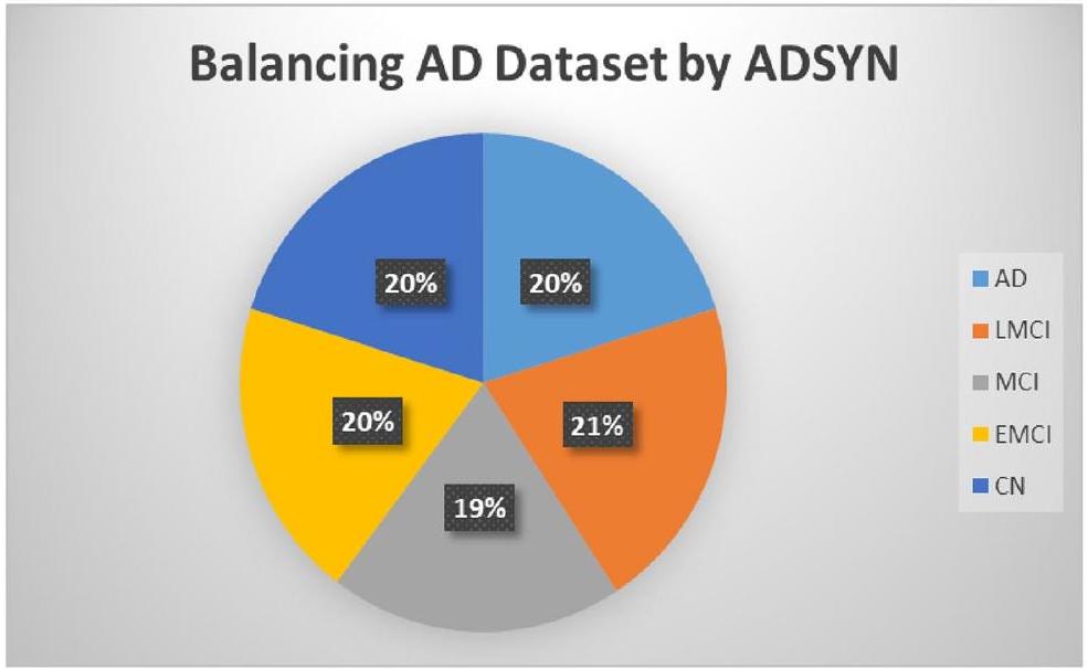
الشكل 3. توزيع الفئات لمجموعة بيانات الرنين المغناطيسي بعد زيادة العينة.
الشكل 4. تمثيل تخطيطي لتقسيم البيانات.
ومعدل التعلم. يمكن أن يساعد الضبط الصحيح للمعلمات في التخفيف من الإفراط في التكيف وزيادة الدقة. بمجرد أن يعمل النموذج بشكل فعال مع مجموعة التحقق، يتوقف عن التدريب بعد فترة محددة لمنع التجارب الزائدة.
عند الانتهاء من عملية التعلم، خضع النموذج للاختبار باستخدام مجموعة اختبار مميزة. ظلت هذه المجموعة الاختبارية غير مستخدمة خلال مرحلة التدريب، مما يضمن عدم وجود تداخل بين بيانات التدريب وبيانات الاختبار. كانت مخصصة فقط لتقييم أداء النموذج، وحساب مقاييس مختلفة مثل الدقة، والموثوقية، والاسترجاع، أو غيرها من مقاييس التقييم التي تقيس قدرة النموذج على التعميم على البيانات غير المرئية.
وصف نموذج CNN المقترح
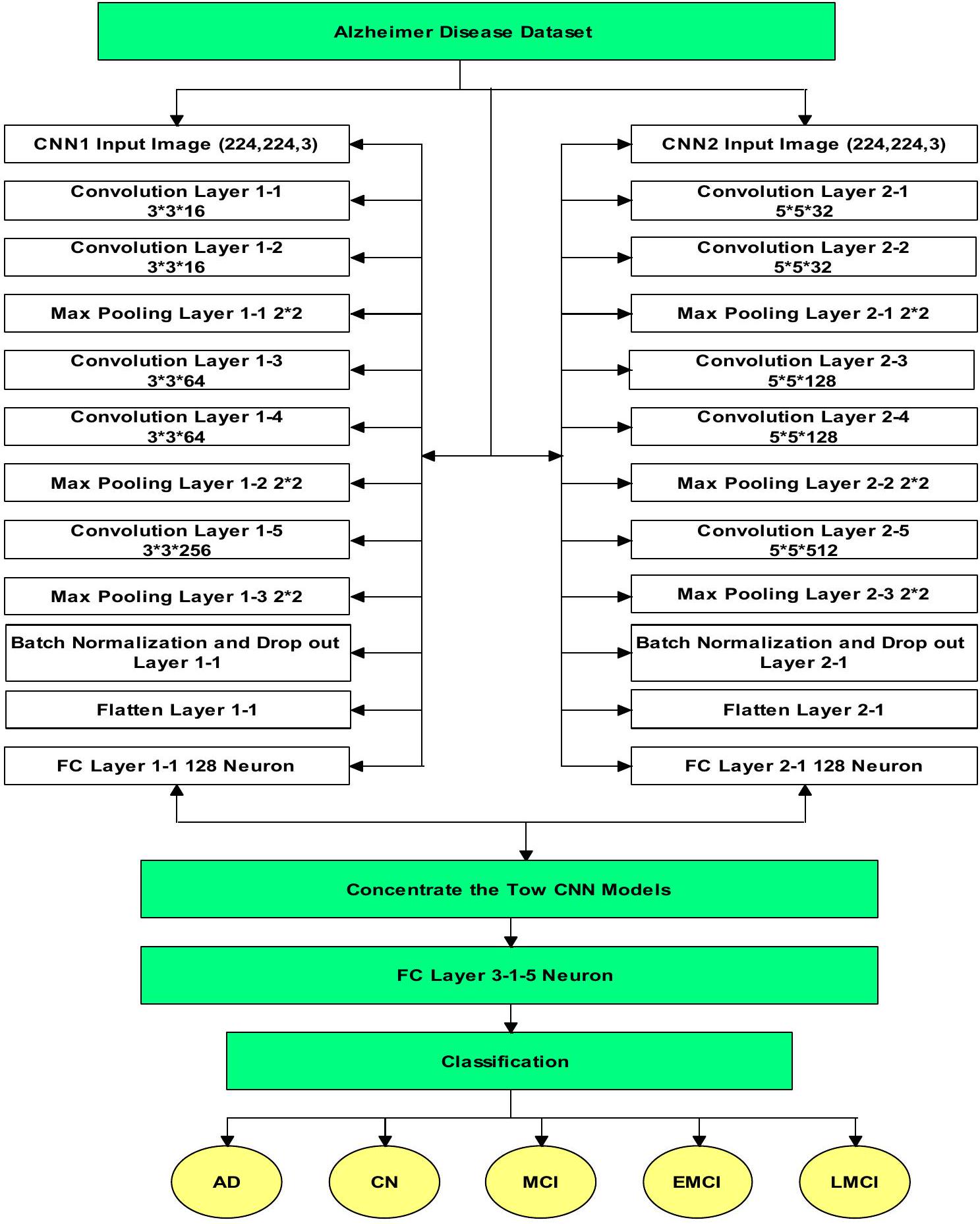
لإجراء معالجة بيانات المرضى المتنوعة، نقوم بإنشاء شبكة تتكون من نموذجين منفصلين من CNN متصلين في طبقة التصنيف، كما هو موضح في الشكل 5.موتر، يمثل البعد الزمني والمحاور (، و z )، يعمل كمدخل للشبكة. يتم بدء نموذج CNN الأول مع طبقتين تلافيفيتين، تحتوي كل منهما على 16 فلتر بحجم .
تستخرج هذه المرشحات الميزات المحلية من الصور المدخلة. بعد ذلك،تُطبق طبقات التجميع الأقصى مع خطوة قدرها 2 لتقليل حجم خرائط الميزات والتقاط المعلومات الأساسية. تتضمن الطبقتان الت convolutional التاليتان كل منهما 64 فلترًا، مما يعزز تمثيل الميزات ذات المستوى الأعلى. يتم تنفيذ جولة أخرى من التجميع الأقصى لتقليل الأبعاد المكانية. بعد ذلك، يتم استخدام طبقة convolutional واحدة مع 256 فلترًا بحجميتم تقديمه لالتقاط الأنماط المعقدة. لمكافحة الإفراط في التكيف، يتم استخدام طبقة إسقاط معتم دمج معدل التعلم، ويتم استخدام تطبيع الدفعات لتطبيع التنشيطات، مما يضمن تحسين استقرار التدريب. أخيرًا، يتم إضافة طبقة متصلة بالكامل تحتوي على 128 خلية عصبية لاستخلاص رؤى عالمية من خرائط الميزات المسطحة.
يتبع النموذج الثاني من CNN هيكلًا مشابهًا ولكن بأحجام فلاتر مختلفة. يبدأ مع طبقتين تلافيفيتين، كل منهما تتكون من 32 فلترًا بحجم. بعد ذلك، تُطبق طبقات التجميع الأقصى مع خطوة قدرها 2. تحتوي الطبقتان التلافيفيتان التاليتان كل منهما على 128 فلترًا بحجميتم تنفيذ جولة لاحقة من التجميع الأقصى لتقليل الأبعاد المكانية. يتبع ذلك طبقة تلافيفية تحتوي على 512 فلترًا بحجم. بالمثل، يتم استخدام طبقة الإسقاط لمنع الإفراط في التكيف، ويتم دمج تطبيع الدفعات لتحسين استقرار التدريب. في النهاية، يتم إضافة طبقة متصلة بالكامل تحتوي على 128 خلية لاستخراج رؤى عالمية من خرائط الميزات.
يتم توليد التنبؤ، الذي يدل على احتمال انتماء المدخلات إلى أي من الفئات الخمس، من خلال دمج الميزات المستخرجة من كل شبكة CNN ومعالجة النتائج على شبكة متصلة بالكامل. ثم يتم تحديد الفئة المتوقعة بناءً على أعلى قيمة. تقدم الجدول 2 وصفًا شاملاً لهندسة الشبكة، موضحًا عمليات كل طبقة تلافيفية، وحجمها، وعدد الفلاتر، والمخرجات. بالإضافة إلى ذلك، يتم تعداد المعلمات لكل طبقة. كل معلمة قابلة للتدريب، مدمجة في عملية الانتشار العكسي، بينما يقوم الجدول 3 بتعداد المعلمات الفائقة لنموذج CNN الذي تم إنشاؤه.
الشكل 5. الهيكل المقترح لشبكة CNN.
تم تقييم العديد من المتغيرات لتحديد ملاءمة الطبقات المختلفة وبعض المعلمات الفائقة المستخدمة في الشبكة. شملت هذه التقييمات تطبيع الدفعات، ومعدلات التسرب المتنوعة، وتقنيات التجميع المتنوعة.
مقاييس تقييم الأداء
تم استخدام مجموعة الاختبار، التي تم إنشاؤها عن طريق تقسيم مجموعة البيانات الأصلية قبل تدريب النموذج، لتقييم النموذج. تم ضمان قوة النموذج باستخدام مقاييس متعددة.تُقاس فعالية تدريب النموذج بمدى شمولية تفسير هذه المؤشرات. استخدمنا مجموعة متنوعة من المؤشرات لتقييم أداء نموذجنا.
طبقة (نوع)
شكل المخرجات
معامل
طبقة الإدخال 1
[(لا شيء، 224، 224، 3)]
0
طبقة الإدخال 2
[(لا شيء، 224، 224، 3)]
0
طبقة الالتفاف 1-1
(لا شيء، 222، 222، 16)
٤٤٨
طبقة الالتفاف 2-1
(لا شيء، 220، 220، 32)
٢٤٣٢
طبقة الالتفاف 1-2
(لا شيء، 220، 220، 16)
2320
طبقة الالتفاف 2-2
(لا شيء، 216، 216، 32)
٢٥,٦٣٢
طبقة تجميع ماكس 1-1
(لا شيء، 110، 110، 16)
0
طبقة تجميع ماكس 2-1
(لا شيء، 108، 108، 32)
0
طبقة الالتفاف 1-3
(لا شيء، 108، 108، 64)
9280
طبقة الالتفاف 2-3
(لا شيء، 104، 104، 128)
١٠٢,٥٢٨
طبقة الالتفاف 1-4
(لا شيء، 106، 106، 64)
٣٦,٩٢٨
طبقة الالتفاف 2-4
(لا شيء، 100، 100، 128)
٤٠٩,٧٢٨
طبقة التجميع الأقصى 1-2
(لا شيء، 53، 53، 64)
0
طبقة تجميع ماكس 2-2
(لا شيء، 50، 50، 128)
0
طبقة الالتفاف 1-5
(لا شيء، 51، 51، 256)
١٤٧,٧١٢
طبقة الالتفاف 2-5
(لا شيء، 46، 46، 512)
1,638,912
طبقة التجميع الأقصى 1-3
(لا شيء، 25، 25، 256)
0
طبقة تجميع ماكس 2-3
(لا شيء، 23، 23، 512)
0
تطبيع الدفعات وطبقة الإسقاط 1-1
(لا شيء، 25، 25، 256)
0
تطبيع الدفعات وطبقة الإسقاط 2-1
(لا شيء، 23، 23، 512)
0
تسطيح الطبقة 1-1
(لا شيء، 160000)
0
تسطيح الطبقة 2-1
(لا شيء، 270848)
0
طبقة FC 1-1
(لا شيء، 128)
٢٠,٤٨٠,١٢٨
طبقة FC 2-1
(لا شيء، 128)
٣٤،٦٦٨،٦٧٢
دمج
(لا شيء، 256)
0
طبقة FC 3-1
(لا شيء، 5)
1285
إجمالي المعلمات: 57,526,005
معاملات قابلة للتدريب: 57,526,005
الجدول 2. معلمات الشبكة العصبية التلافيفية المقترحة.
الدقة: تمثل الدقة النسبة المئوية للتوقعات الفعلية التي تم التنبؤ بها بشكل صحيح. بشكل عام، القيم التي تزيد عنتعتبر جيدة، بينما القيم التي تتجاوزتعتبر ممتازة. يتم تحديد هذه المقياس من خلال التعبيرات التالية.
أين،هي القيم الصحيحة الإيجابية، الصحيحة السلبية، الخاطئة السلبية، والخاطئة الإيجابية، على التوالي. 2. الدقة: يتم استخدام المعادلة التالية لحساب الدقة، والتي تُعرف بأنها نسبة التوقعات المتفائلة الدقيقة إلى جميع التوقعات المتفائلة.. بشكل عام، قيم الدقة تتجاوز تعتبر مرضية.
الاسترجاع: يمكن الإشارة إليه أيضًا بمعدل الحساسية أو معدل الإيجابيات الحقيقية. يتضمن الاسترجاع مقارنة التوقعات الإيجابية الدقيقة مع جميع الإيجابيات الصحيحة الفعلية.تتراوح قيم الاسترجاع المقبولة عادةً من 70 إلىتُستخدم المعادلة التالية لحساب الاسترجاع:
درجة F1: تعتبر درجة F1 مميزة لأنها توفر قيمة مميزة لكل تصنيف.استخدم الحساب التالي لتحديد درجة F1.
الدقة المتوازنة: يتم حسابها عن طريق متوسط معدل الإيجابيات الحقيقية (TPR) ومعدل السلبيات الحقيقية (TNR). يمثل TPR نسبة الأحداث الإيجابية إلى الأحداث السلبية التي تم تحديدها بدقة، بينما يشير TNR إلى نسبة الأحداث السلبية إلى الأحداث الإيجابية..
معامل ارتباط ماثيوز (MCC): يعتبر MCC مقياسًا أكثر تعقيدًا يأخذ في الاعتبار عدم التوازن بين الأمثلة الإيجابية والسلبية في مجموعة البيانات. إذا كانت إحدى الفئات تفوق الأخرى بشكل كبير في التكرارات، فقد يصبح المقياس غير متوازن.يتم حساب MCC على النحو التالي:
تطوير النموذج والتدريب
في عملنا، قمنا بتدريب وتصديق المصنف باستخدام برامج مفتوحة المصدر: بايثون 3.0 ومنصة جوجل كولابوراتوري برو.مزود بوحدة معالجة الرسوميات:تيسلا K80، التي تحتوي على 2496 نواة CUDA وقدرة حسابية تبلغ 3.7. لديها 12 جيجابايت من ذاكرة الوصول العشوائي GDDR5 (11.439 جيجابايت قابلة للاستخدام). لتطوير النموذج المقترح، اخترنا استخدام مكتبة Keras المدمجة مع وحدات TensorFlow. بالإضافة إلى ذلك، استخدمنا مكتبات بايثون مثل Scikit-learn وNumpy وOpenCV كمكتبات بايثون.
التجارب والنتائج
في القسم التالي، نتعمق في خطوات التجربة، نقدم النتائج، ونقارنها بالنتائج السابقة.
كما هو موضح في الشكل 2، بعد تحميل بيانات MRI من ADNI، قمنا بتعزيز الصور واستخدمنا نهج ADASYN لمعالجة عدم توازن البيانات. زاد حجم مجموعة البيانات إلى 3000 صورة بعد تطبيق ADASYN. بعد ذلك، قمنا بتقسيم البيانات إلى ثلاث مجموعات بناءً على النسب الموضحة في الشكل 3: مجموعات التدريب، والتحقق، والاختبار. في النهاية، استخدمنا بيانات التدريب لتدريب النموذج المقترح.
يتكون النموذج المقترح من شبكتين عصبيتين تلافيفيتين متميزتين تم دمجهما في مرحلة التصنيف. قمنا بتطبيق مجموعة بيانات التصوير بالرنين المغناطيسي متعددة الفئات ذات الخمس طرق على كل شبكة بشكل فردي. تم استخدام مقاييس مثل الدقة، والاسترجاع، والدقة، والدقة المتوازنة، ومعامل ارتباط ماثيو، ودالة الخسارة لتقييم الأداء. ثم تم مقارنة أداء هذه الشبكات الفردية مع أداء الشبكة العصبية التلافيفية المدمجة، كما هو موضح في الجدول 4.
تقدم الجداول 5 و6 و7 نتائج أداء التصنيف لهذه الشبكات العصبية التلافيفية، مع التركيز على مقاييس مثل الاسترجاع والدقة ودرجات f1 والدعم، حيث يشير ‘الدعم’ إلى عدد العينات.
كما ترى، يمكن أن يؤدي تقليل حجم الفلتر إلى تحسين نتائج التصنيف. على وجه التحديد، يستخدم CNN2 حجم الفلتر، يحتاج إلى استخدام ضعف عدد الفلاتر الموجودة في CNN1 (الذي يستخدم حجم الفلتر) لتحقيق دقة قابلة للمقارنة مع CNN1. علاوة على ذلك، عندما يتم دمج الشبكتين، تظهر الشبكة الناتجة دقة أعلى من أي من الشبكتين الفرديتين. تنشأ هذه التحسينات لأن الشبكتين تكملان بعضهما البعض، حيث تقدمان وجهات نظر مختلفة حول البيانات.
لتقييم فعالية هذا النهج عبر مهام التصنيف المختلفة، قمنا بتطبيق الشبكة المدمجة على مجموعات البيانات، مقدّمين نتائج تجريبية لمشكلة تصنيف متعددة الفئات بخمس فئات كمعيار.مشكلة تصنيف متعددة الفئات بأربعة طرق كمعيارومشكلة تصنيف ثلاثية معيارية.
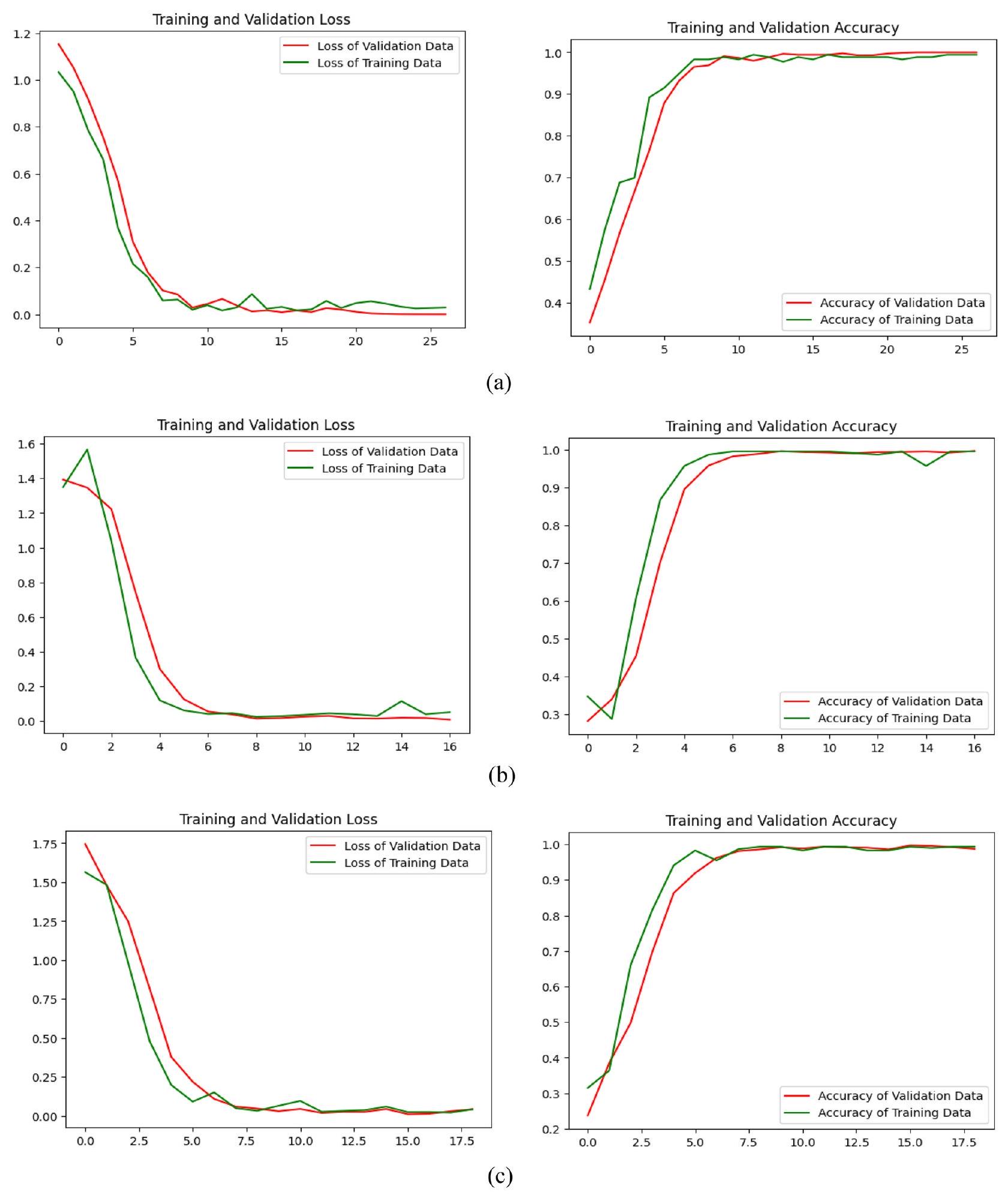
في الشكل 6، نعرض في البداية الرسوم البيانية التي تقارن دقة تدريب النموذج المقترح مقابل دقة التحقق، بالإضافة إلى خسارة التدريب مقابل خسارة التحقق، لمشاكل التصنيف المتعدد ثلاثية الاتجاهات وأربعة الاتجاهات وخمسة الاتجاهات. الجدول 8 يقارن أداء النموذج المقترح عبر المشاكل المتعددة المذكورة.
المقاييس
سي إن إن 1
سي إن إن 2
مقترح
خسارة
0.3286
0.1491
0.0325
دقة
استدعاء
دقة
الدقة المتوازنة
معامل ارتباط ماثيو
الجدول 4. أداء أول شبكة عصبية تلافيفية تم تطويرها، وثاني شبكة عصبية تلافيفية تم تطويرها، والنموذج المقترح لبيانات الاختبار.
فصول
دقة
استدعاء
درجة F1
دعم
م.ع
0.98
1.00
0.99
63
CN
0.90
0.91
0.90
٥٧
EMCI
0.95
0.98
0.96
53
LMCI
1.00
1.00
1.00
53
MCI
0.94
0.88
0.91
٥٨
الجدول 5. نتيجة الدقة والاسترجاع ودرجة F1 لكل فئة عند تطبيق شبكة CNN المطورة الأولى فقط على بيانات الاختبار لتصنيفها إلى 5 فئات.
فصول
دقة
استدعاء
درجة F1
دعم
م.ع
0.98
1.00
0.99
63
CN
0.93
0.95
0.94
57
EMCI
0.96
0.89
0.92
53
LMCI
1.00
1.00
1.00
52
MCI
0.92
0.95
0.93
٥٩
الجدول 6. نتيجة الدقة، الاسترجاع، ودرجة F1 لكل فئة عند تطبيق الشبكة العصبية التلافيفية الثانية المطورة فقط على بيانات الاختبار لتصنيفها إلى 5 فئات.
فصول
دقة
استدعاء
درجة F1
دعم
م.ع
0.98
1.00
0.99
٥٨
CN
0.93
0.95
0.94
٥٩
EMCI
0.96
0.89
0.92
٥٦
LMCI
1
1
1
٥٥
MCI
0.92
0.95
0.93
٥٨
الجدول 7. نتيجة الدقة، الاسترجاع، ودرجة F1 لكل فئة عند تطبيق الشبكة العصبية الالتفافية المقترحة على بيانات الاختبار لتصنيفها إلى 5 فئات.
مصفوفة الالتباس
يتم استخدامه لتقييم وحساب مقاييس نماذج التصنيف المختلفة. يوفر تحليلًا رقميًا لتوقعات النموذج خلال مرحلة الاختبار..
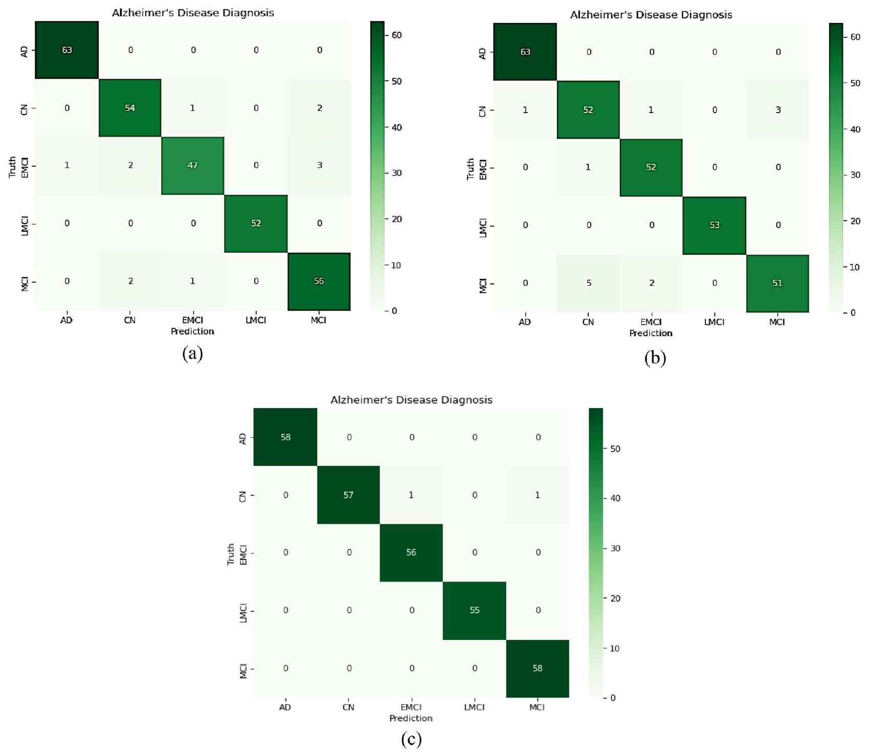
تم تطوير مصفوفة الارتباك للنموذج المقترح، كما هو موضح في الأشكال 7 و 8، لتقييم مدى أداء الشبكة المقترحة في كل فئة من بيانات الاختبار. بالإضافة إلى ذلك، توفر الجداول 7 و 9 و 10 تفاصيل حول تقرير تصنيف الفئات للنموذج المقترح استنادًا إلى الدقة والاسترجاع ودرجة F1.
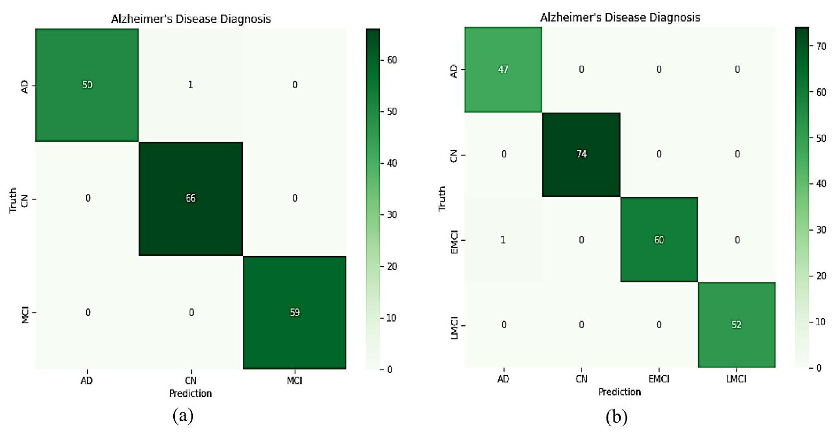
الشكل 7c يظهر أن أحد الأفراد من CN تم تصنيفه بشكل خاطئ كـ EMCI، وآخر تم تصنيفه بشكل خاطئ كـ MCI في حالة خمس تصنيفات متعددة الفئات. وهذا يدل على نموذج مؤثر لأنه في التشخيص الطبي، يُفضل تصنيف الشخص كمريض على استبعاد شخص مريض من خلال التنبؤ الخاطئ بالسلبية. كما هو موضح في الشكل 8، تم تشخيص أحد الأفراد من EMCI بشكل غير صحيح بأنه مصاب بـ AD في أربع تصنيفات متعددة الفئات. تم تصنيف أحد EMCI بشكل خاطئ كـفي تصنيف ثلاثي الاتجاهات.
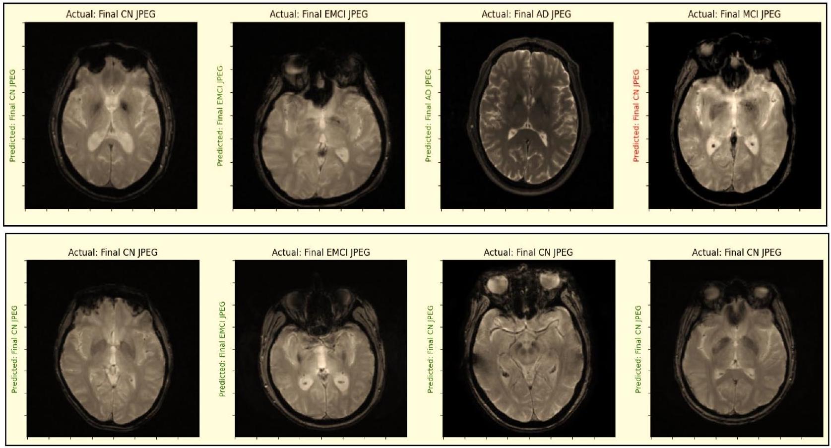
بالنسبة لتصنيفات الثلاثية، الرباعية، والخماسية، حقق النموذج المقترح قيم دقة متوسطة قدرها، “، و ، على التوالي. بالإضافة إلى ذلك، كما هو موضح في الشكل 9، تم فحص النموذج المقترح لتحديد ما إذا كانت التسمية المتوقعة تتطابق مع التسمية الفعلية.
تحليل GRAD-CAM
في السعي المستمر لفهم واستغلال قوة التعلم العميق، تكمن تحديات حاسمة في جعل هذه الشبكات العصبية المعقدة أكثر قابلية للتفسير. هذا أمر بالغ الأهمية بشكل خاص في التطبيقات مثل تصوير الطب، حيث الثقة والفهم هما الأساس. يمكن عرض التعلم العميق في العمل من خلال رسم خرائط تنشيط الفئة المدعومة بالتدرج (Grad-CAM)، الذي تم تطويره بواسطة سيلفراجو وآخرين.. هذه التقنية العبقرية تعمل كعدسة مكبرة للشبكات العصبية العميقة، حيث توفر تمثيلاً بصرياً لآليات عملها الداخلية. إنه مثل التلصص خلف الستار لرؤية ما تركز عليه هذه الخوارزميات عند تحليل البيانات. تعتبر صورة الرنين المغناطيسي المدخل للنموذج المقترح، والذي يستخدم كطريقة للكشف. يتم تطبيق Grad-CAM على آخر طبقة تلافيفية من النموذجين المقترحين من CNN قبل استخدام الدمج للحصول على التسمية المتوقعة. يتم استخراج خريطة الميزات للشبكة المقترحة في هذه الحالة باستخدام تقنية Grad-CAM. تُظهر خريطة الحرارة منطقة الصورة التي تعتبر أساسية لتحديد الفئة المستهدفة كتجسيد بصري لشبكة مقترحة. علاوة على ذلك، فإن أهمية كل نموذج CNN في اتخاذ القرار وكذلك تأثير
يمكن تحديد تغيير حجم وكمية الفلاتر في كل نموذج بهذه الطريقة. تُظهر الخرائط الحرارية والتصورات التي تم إنشاؤها من خلال تطبيق خوارزمية GRAD-CAM على صور الأشعة السينية للـ AD و CN و MCI في الشكل 10. هذه الأدلة البصرية لا تعزز فقط فهمنا لتوقعات النموذج، بل تمهد أيضًا الطريق للتحقق من تشخيص مرض الزهايمر بثقة أكبر.
المقاييس
ثلاثي الاتجاهات متعدد الفئات
أربعة اتجاهات متعددة الفئات
خماسي متعدد الفئات
خسارة
0.0163
0.0414
0.0325
دقة
99.43%
99.57%
99.30%
استدعاء
99.43%
99.57%
99.30%
دقة
99.43%
99.57%
99.30%
الدقة المتوازنة
99.35%
99.57%
99.32%
معامل ارتباط ماثيو
99.15%
99.43%
99.13%
الجدول 8. أداء النموذج المقترح مع تصنيف متعدد الفئات ثلاثي الاتجاهات؛ تصنيف متعدد الفئات رباعي الاتجاهات؛ وتصنيف متعدد الفئات ثلاثي الاتجاهات.
الشكل 7. مصفوفة الالتباس للنموذج المقترح على بيانات الاختبار (أ) CNN1؛ (ب) CNN2؛ (ج) الشبكة العصبية التلافيفية المطورة بشكل عام.
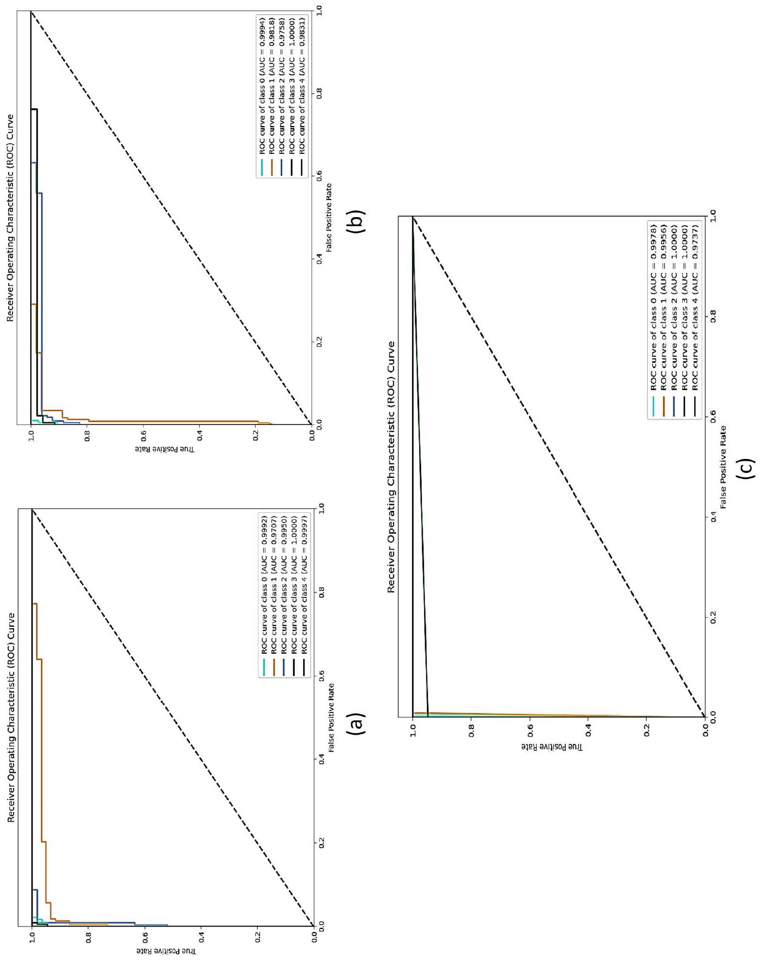
تحليل منحنى ROC
يتم تقييم أداء النموذج المقترح من خلال حساب قيم AUC (المساحة تحت المنحنى) وROC (منحنى خصائص التشغيل المستقبلية).تُستخدم طريقة الفئة الواحدة مقابل البقية في التصنيف متعدد الفئات. تُبنى منحنيات ROC باستخدام 1 – الخصوصية (معدل الإيجابيات الكاذبة) كالمحور السيني والحساسية (معدل الإيجابيات الحقيقية) كالمحور الصادي. حساب المساحة تحت منحنى ROC يعطي نتيجة AUC. تتراوح قيمة AUC من 0 إلى 1. تنخفض أداء النموذج كلما اقتربت القيمة من 0. وبالمثل، كلما اقتربت القيمة من 1، زادت كفاءة النموذج.
الشكل 8. مصفوفة الالتباس للنموذج المقترح على بيانات الاختبار (أ) 5 فئات متعددة؛ (ب) 4 فئات متعددة.
فصول
دقة
استدعاء
درجة F1
دعم
م.ع
1.00
0.98
0.99
51
CN
0.99
1.00
0.99
66
MCI
1.00
1.00
1.00
٥٩
الجدول 9. نتيجة الدقة والاسترجاع ودرجة F1 لكل فئة عند تطبيق الشبكة العصبية التلافيفية المقترحة على بيانات الاختبار لتصنيفها إلى 3 فئات.
فصول
دقة
استدعاء
درجة F1
دعم
م
0.98
1.00
0.99
٤٧
CN
1.00
1.00
1.00
74
EMCI
1.00
0.98
0.99
61
LMCI
1.00
1.00
1.00
52
الجدول 10. نتيجة الدقة، الاسترجاع، ودرجة F1 لكل فئة عند تطبيق الشبكة العصبية التلافيفية المقترحة على بيانات الاختبار لتصنيفها إلى 4 فئات.
تظهر الشكل 10 منحنيات ROC للنماذج الأولى والثانية والمقترحة من CNN عبر الفئات الخمس. مع الأخذ في الاعتبار أن الفئات، و 5 تشير إلى CN و MCI و AD و LMCI و EMCI، على التوالي. من خلال فحص الشكل 11، يمكن ملاحظة أن النموذج المقترح قد حسّن بشكل كبير قيم AUC لجميع فئات مرض الزهايمر. قيمة AUC لفئة CN هي هو هو القيمة هي 1، وEMCI هي 0.9737. بينما كانت قيم AUC عند تطبيق CNN1 المقترح كما يلي: الفئة CN هي 0.9978، MCI هي 0.9956، AD هي 0.9950، LMCI هي 1، وEMCI هي 0.9997. بينما كانت قيم AUC عند تطبيق CNN 2 المقترح 0.9994 لـ CN، 0.9818 لـ MCI، 0.9758 لـ AD، 1 لـ LMCI، و0.9831 لـ EMCI. لذلك، فإن النموذج المقترح هو طريقة أكثر دقة وموثوقية لتشخيص مرض الزهايمر.
اختبار ويلكوكسون للرتب الموقعة
لضمان أن النتائج لم تكن مجرد نتيجة للصدفة العشوائية، تم إجراء تحليل إحصائي للدلالة (S). تم حساب قيم p لكل نموذج، واستخدم الباحثون اختبار ويلكوكسون للرتب الموقعة لهذا الغرض. يُستخدم اختبار ويلكوكسون للرتب الموقعة عادةً عند مقارنة متغيرين غير معلميّن. من خلال هذا الاختبار، يتم مقارنة عينتين مستقلتين لتقييم الفروق الزوجية عبر ملاحظات متعددة من مجموعة بيانات واحدة. تشير النتيجة إلى ما إذا كان هناك تمييز في متوسط رتب السكان. قيم p للمقارنات الزوجية للنماذجمفصلة في الجدول 11. مقارنة بـ
الشكل 9. فحص ما إذا كانت التسمية المتوقعة تتطابق مع التسمية الحقيقية أم لا.
الشكل 10. خوارزمية GRAD-CAM عند تطبيقها على صور أشعة الرنين المغناطيسي لحالات مرض الزهايمر، والحالة الطبيعية، والاعتلال المعرفي المعتدل.
الشكل 11. منحنى ROC وقيمة AUC لـ (أ) CNN1، (ب) CNN2، و(ج) النموذج المقترح.
لا.
مقارنات ثنائية نموذجية
قيمة p
1
النموذج المقترح مقابل AlexNet
0.007280
2
النموذج المقترح مقابل ResNet50
0.001655
٣
النموذج المقترح مقابل Xception
0.007157
٤
النموذج المقترح مقابل VGG16
0.002338
الجدول 11. اختبار ويلكوكسون للرتب الموقعة.
نموذج المقترح أظهر أداءً متفوقًا مقارنة بالنماذج الأخرى. في جوهره، تفوق النموذج المقترح بشكل كبير على النماذج الأربعة الأخرى، كما يتضح من فرق قيمة p بين النموذج المقترح والنماذج الأخرى الذي كان أقل من 0.05.
نقاش
كشفت النتائج أن النموذج المقترح يميز بدقة بين الفئات الثلاثية (AD/ MCI/CN) والفئات الرباعية (AD/CN/LMCI/EMCI) والفئات الخماسية (AD/CN/LMCI/EMCI/MCI) لمرض الزهايمر.
لقد استخدمت العديد من الدراسات منهجيات مختلفة لتصنيف مراحل مرض الزهايمر. كما هو موضح في الجدول 12، قمنا بمقارنة أداء النظام المقترح مع نماذج مختلفة تم مناقشتها في مراجعة الأدبيات.
من الواضح أن النهج الموصى به حقق أفضل النتائج من حيث الدقة وأدى أداءً استثنائيًا في مشاكل التصنيف المتعدد الفئات 3-way و4-way و5-way. بالإضافة إلى ذلك، تؤكد النتائج على أهمية دمج نماذج CNN متعددة في طبقة التصنيف لتعزيز القدرة التمييزية للنموذج. مقارنةً بتقنيات النماذج الفردية، يتفوق طريقتنا في التقاط الأنماط المتعلقة بمرض الزهايمر من خلال دمج البيانات التكميلية من CNNs مختلفة.
تقدم الطريقة المقترحة عدة مزايا مقارنة بالطرق التقليدية للكشف المبكر عن مرض الزهايمر:
المؤلفون
علامة حيوية
قاعدة بيانات
المنهجية
تصنيف
دقة
رمضان وآخرون (2020)
الرنين المغناطيسي
أدني
ريزنت 18 (تعديل دقيق)
5 طرق AD/CN/MCI/EMCI/LMCI
97.88%
بارمار وآخرون (2020)
الرنين المغناطيسي
أدني
شبكة عصبية تلافيفية ثلاثية الأبعاد
4 طرق AD/CN/EMCI/LMCI
93.00%
بويتي-كاسترو وآخرون (2020)
الرنين المغناطيسي
أدني
ريزنت18 و SVM
3 طرق AD/CN/MCI
78.72%
فؤادة وآخرون (2021)
الرنين المغناطيسي
أدني
أليكس نت
4 طرق AD/CN/EMCI/LMCI
95%
موروجان وآخرون (2021)
الرنين المغناطيسي
أدني
سي إن إن
4 طرق AD/CN/EMCI/LMCI
95.23%
بوفانيشوري وآخرون (2021)
المورفومترية المعتمدة على الفوكسل (VBM)
أدني
في جي جي نت غوغل نت ريس نت
تصنيف ثنائي NC/AD
٩٦٫٠٨٪ ٩٧٫١٥٪ ٩٤٫٦٠٪
أودوسامي وآخرون (2022)
الرنين المغناطيسي
أدني
Resnet18 و DenseNet121 مع وزن عشوائي
3 طرق AD/CN/MCI
98.21%
4 طرق AD/CN/EMCI/LMCI
93.06%
5 طرق AD/CN/MCI/EMCI/LMCI
98.86%
نو وآخرون (2023)
التصوير بالرنين المغناطيسي الوظيفي
أدني
نموذج تصنيف 3D-CNN-LSTM
4 طرق AD/CN/EMCI/LMCI
96.43%
تشيلبي وآخرون (2023)
المورفومترية المعتمدة على التنسور (TBM)
أدني
كتلة كثيفة عميقة تعتمد على بنية Xception
3 طرق AD/CN/MCI
95.81%
أكتير وآخرون (2023)
الرنين المغناطيسي
أدني
إنسيبشن V3 (التعديل الدقيق)
6 طرق AD/CN/SMC/MCI/EMCI/LMCI
98.68%
بامبر وآخرون، (2023)
الرنين المغناطيسي
أواسيز-3
سي إن إن
4 طرق AD/CN/MCI/ MCI معتدل
98%
مقترح
الرنين المغناطيسي
أدني
سي إن إن
3 طرق AD/CN/MCI
99.43%
4 طرق AD/CN/EMCI/LMCI
99.57%
5 طرق AD/CN/MCI/EMCI/LMCI
الجدول 12. مقارنة أداء التصنيف.
بينما تميز معظم أساليب التصنيف بين صور مرض الزهايمر (AD) وصور الأفراد الأصحاء (CN) أو بين مرض الزهايمر (AD) ومرض الاعتلال المعرفي المعتدل (MCI)، تستخدم دراستنا تصنيفات متعددة الفئات بثلاثة وأربعة وخمسة طرق.
تركز جهودنا على التشخيص المبكر لمرض الزهايمر، من خلال تعزيز دقة التمييز بين ضعف الإدراك المعتدل، وضعف الإدراك المعتدل المبكر، وضعف الإدراك المعتدل المتأخر، والأشخاص الأصحاء.
بصرف النظر عن بيانات التدريب، استخدمنا مجموعات مستقلة من الصور لتقييم نموذجنا.
التقنية المقترحة غير جراحية وقابلة للتطبيق على فحوصات الرنين المغناطيسي، والتي تُستخدم عادة في البيئات السريرية.
نهجنا يقضي على الحاجة لاستخراج الميزات يدويًا، وهي مهمة تتطلب جهدًا كبيرًا وتكون ذات طابع شخصي.
علاوة على ذلك، يمكن للطريقة المقترحة استخراج ميزات معقدة من صور الرنين المغناطيسي التي يصعب استخراجها باستخدام الطرق التقليدية.
ومع ذلك، فإن النهج المقترح له بعض القيود. أولاً، تم استخدام مجموعة بيانات التصوير بالرنين المغناطيسي ADNI لتقييم طريقتنا. لكي يكون الاستراتيجية المقترحة قابلة للتطبيق بشكل عالمي، يجب اختبارها على مجموعات بيانات إضافية. البيانات الواسعة المطلوبة لتدريب الشبكات العصبية التلافيفية في نهجنا قد تحد من قابليتها السريرية في السيناريوهات التي تكون فيها البيانات نادرة. أخيرًا، لا يتضمن النموذج بيانات سريرية؛ بل يساعد الأطباء في اتخاذ القرارات دون استبدالها.
في الختام، تقدم استراتيجيتنا المقترحة طريقًا واعدًا للكشف المبكر عن مرض الزهايمر. يمكن أن تسهل هذه الطريقة تشخيص مرض الزهايمر بشكل أكثر timely وفعالية، مما يؤدي إلى تحسين النتائج العلاجية.
الخاتمة
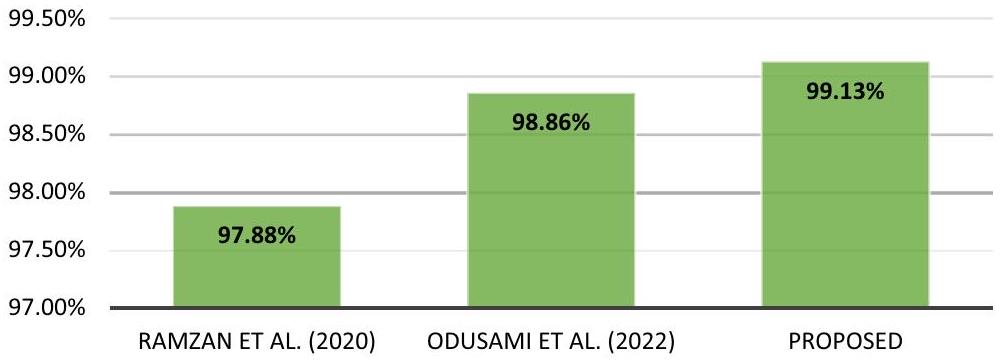
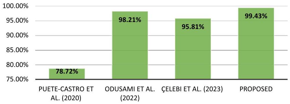
باختصار، تقترح هذه البحث طريقة جديدة للكشف المبكر عن مرض الزهايمر (AD) باستخدام بيانات التصوير بالرنين المغناطيسي (MRI). تعتمد الطريقة المقترحة على استخدام شبكتين عصبيتين تلافيفيتين (CNNs) وتجمع مخرجاتهما من خلال دمجهما في طبقة التصنيف. الهدف هو التقاط ميزات مكانية وبنائية متنوعة للدماغ، مما يسهل التحليل الشامل للأنماط المتعلقة بمرض الزهايمر. يتم إثبات فعالية نهجنا من خلال النتائج التجريبية على مجموعة بيانات ADNI، مقارنةً بالنتائج من الأبحاث السابقة، كما هو موضح في الأشكال 12 و 13 و 14. بالنسبة لمهام التصنيف ذات الثلاثة اتجاهات، الأربعة اتجاهات، والخمسة اتجاهات، حققنا معدلات دقة مرتفعة بشكل ملحوظ من، و على التوالي. بشكل عام، تعزز هذه الدراسة مجال اكتشاف مرض الزهايمر من خلال تقديم نهج مبتكر مع نتائج دقة واعدة. الطريقة المقترحة لديها القدرة على مساعدة الأطباء والباحثين في تشخيص مرض الزهايمر في وقت مبكر، مما يمهد الطريق
دقة التصنيف المتعدد 5 طرق
الشكل 12. مقارنة دقة طرق التصنيف المتعددة 5.
دقة التصنيف المتعدد 4 طرق
الشكل 13. مقارنة دقة طرق التصنيف المتعددة 4 – طرق.
دقة التصنيف المتعدد 3 – طرق
الشكل 14. مقارنة دقة طرق التصنيف المتعددة 3 – طرق.
للعلاجات الاستباقية وتحسين نتائج المرضى. ستركز الجهود المستقبلية على التحقق من صحة الطريقة باستخدام مجموعات بيانات أكبر، واستكشاف قابليتها للتطبيق في الإعدادات السريرية، ودمج بيانات إضافية لتعزيز الدقة
توفر البيانات
بيانات التصوير بالرنين المغناطيسي المستخدمة في بحثي متاحة للجمهور من قاعدة بيانات مبادرة التصوير العصبي لمرض الزهايمر (ADNI) .
توفر الشيفرة
الشيفرة بلغة بايثون المستخدمة في المعالجة متاحة عند الطلب.
تاريخ الاستلام: 17 أكتوبر 2023؛ تاريخ القبول: 4 فبراير 2024
تم النشر على الإنترنت: 12 فبراير 2024
References
Mohamed, T. M. et al. Alzheimer’s disease improved through the activity of mitochondrial chain complexes and their gene expression in rats by boswellic acid. Metab. Brain Dis. 36(2), 255-264. https://doi.org/10.1007/s11011-020-00639-7 (2021).
Tadokoro, K. et al. Early detection of cognitive decline in mild cognitive impairment and Alzheimer’s disease with a novel eye tracking test. J. Neurol. Sci. 427, 117529. https://doi.org/10.1016/j.jns.2021.117529 (2021).
Zhang, T. et al. Predicting MCI to AD conversation using integrated sMRI and rs-fMRI: Machine learning and graph theory approach. Front. Aging Neurosci. 2021, 13. https://doi.org/10.3389/fnagi.2021.688926 (2021).
Feng, C. et al. Deep learning framework for Alzheimer’s disease diagnosis via 3D-CNN and FSBi-LSTM. IEEE Access 7, 6360563618 (2019).
Forouzannezhad, P. et al. A deep neural network approach for early diagnosis of mild cognitive impairment using multiple features. In 2018 17th IEEE international conference on machine learning and applications (ICMLA), IEEE (2018).
Segovia, F. et al. Multivariate analysis of dual-point amyloid PET intended to assist the diagnosis of Alzheimer’s disease. Neurocomputing 417, 1-9 (2020).
Bharati, P. & Pramanik, A. Deep learning techniques-R-CNN to mask R-CNN: Asurvey. Comput. Intel. Pattern Recogn. Proc. CIPR 2020, 657-668 (2019).
Abd-Ellah, M. K. et al. A review on brain tumor diagnosis from MRI images: Practical implications, key achievements, and lessons learned. Magn. Reson. Imaging 61, 300-318 (2019).
Siuly, S. & Zhang, Y. Medical big data: Neurological diseases diagnosis through medical data analysis. Data Sci. Eng. 1, 54-64 (2016).
Ghaffari-Rafi, A. et al. The role of magnetic resonance imaging to inform clinical decision-making in acute spinal cord injury: A systematic review and meta-analysis. J. Clin. Med. 10(21), 4948 (2021).
Salarian, M. et al. Early detection and staging of chronic liver diseases with a protein MRI contrast agent. Nat. Commun. 10(1), 4777 (2019).
Chaddad, A., Desrosiers, C. & Niazi, T. Deep radiomic analysis of MRI related to Alzheimer’s disease. IEEE Access 6, 58213-58221 (2018).
Teipel, S. J. et al. Multicenter resting state functional connectivity in prodromal and dementia stages of Alzheimer’s disease. J. Alzheim. Dis. 64(3), 801-813 (2018).
Shakarami, A., Tarrah, H. & Mahdavi-Hormat, A. A CAD system for diagnosing Alzheimer’s disease using 2D slices and an improved AlexNet-SVM method. Optik 212, 164237 (2020).
Qiu, S. et al. Development and validation of an interpretable deep learning framework for Alzheimer’s disease classification. Brain 143(6), 1920-1933 (2020).
Ramzan, F. et al. A deep learning approach for automated diagnosis and multi-class classification of Alzheimer’s disease stages using resting-state fMRI and residual neural networks. J. Med. Syst. 44, 1-16 (2020).
Amin-Naji, M., Mahdavinataj, H. & Aghagolzadeh, A. Alzheimer’s disease diagnosis from structural MRI using Siamese convolutional neural network. In 2019 4th international Conference on Pattern Recognition and Image Analysis (IPRIA), IEEE (2019).
Jabason, E., Ahmad, M. O. & Swamy, M. Classification of Alzheimer’s disease from MRI data using an ensemble of hybrid deep convolutional neural networks. In 2019 IEEE 62nd International Midwest Symposium on Circuits and Systems (MWSCAS), IEEE (2019).
Odusami, M. et al. Comparable study of pre-trained model on alzheimer disease classification. In Computational Science and Its Applications-ICCSA 2021: 21st International Conference, Cagliari, Italy, September 13-16, 2021, Proceedings, Part V 21 (Springer, 2021).
Fuadah, Y. N. et al. Automated classification of alzheimer’s disease based on MRI image processing using convolutional neural network (CNN) with AlexNet architecture. J. Phys. Conf. Ser. 1844(1), 012020. https://doi.org/10.1088/1742-6596/1844/1/012020 (2021).
Odusami, M., Maskeliūnas, R. & Damaševičius, R. An intelligent system for early recognition of Alzheimer’s disease using neuroimaging. Sensors 22(3), 740 (2022).
Liu, M. et al. A multi-model deep convolutional neural network for automatic hippocampus segmentation and classification in Alzheimer’s disease. Neuroimage 208, 116459 (2020).
Cheng, B. et al. Domain transfer learning for MCI conversion prediction. IEEE Trans. Biomed. Eng. 62(7), 1805-1817 (2015).
Li, F. et al. A robust deep model for improved classification of AD/MCI patients. IEEE J. Biomed. Health Inf. 19(5), 1610-1616 (2015).
Qi, C. R. et al. Volumetric and multi-view cnns for object classification on 3d data. In Proceedings of the IEEE Conference on Computer Vision and Pattern Recognition (2016).
Yadav, K. S. & Miyapuram, K. P. A novel approach towards early detection of alzheimer’s disease using deep learning on magnetic resonance images. In Brain Informatics: 14th International Conference, BI 2021, Virtual Event, September 17-19, 2021, Proceedings 14 (Springer, 2021).
Buvaneswari, P. & Gayathri, R. Deep learning-based segmentation in classification of Alzheimer’s disease. Arab. J. Sci. Eng. 46, 5373-5383 (2021).
Parmar, H. et al. Spatiotemporal feature extraction and classification of Alzheimer’s disease using deep learning 3D-CNN for fMRI data. J. Med. Imaging 2020, 7. https://doi.org/10.1117/1.JMI.7.5.056001 (2020).
Çelebi, S. B. & Emiroğlu, B. G. A novel deep dense block-based model for detecting Alzheimer’s Disease. Appl. Sci. 13(15), 8686 (2023).
Salehi, W., Baglat, P. & Gupta, G. Multiple machine learning models for detection of alzheimer’s disease using OASIS dataset. IFIP Adv. Inf. Commun. Technol. 617, 614-622. https://doi.org/10.1007/978-3-030-64849-7_54 (2020).
Salehi, A. W., Baglat, P. & Gupta, G. Alzheimer’s disease diagnosis using deep learning techniques. Int. J. Eng. Adv. Technol 9(3), 874-880 (2020).
Murugan, S. et al. DEMNET: A deep learning model for early diagnosis of Alzheimer diseases and dementia from MR images. IEEE Access 9, 90319-90329 (2021).
Noh, J.-H., Kim, J.-H. & Yang, H.-D. Classification of alzheimer’s progression using fMRI data. Sensors 23(14), 6330 (2023).
Rallabandi, S., Tulpule, K. & Gattu, M. Automatic classification of cognitively normal, mild cognitive impairment and Alzheimer’s disease using structural MRI analysis. Inf. Med. Unlock. 18, 100305. https://doi.org/10.1016/j.imu.2020.100305 (2020).
Bamber, S. S. & Vishvakarma, T. Medical image classification for Alzheimer’s using a deep learning approach. J. Eng. Appl. Sci. 70(1), 54 (2023).
Shamrat, F. J. M. et al. AlzheimerNet: An effective deep learning based proposition for alzheimer’s disease stages classification from functional brain changes in magnetic resonance images. IEEE Access 11, 16376-16395 (2023).
Kauderer-Abrams, E., Quantifying translation-invariance in convolutional neural networks. arXiv:1801.01450 (2017).
De, A. & Chowdhury, A. S. DTI based Alzheimer’s disease classification with rank modulated fusion of CNNs and random forest. Expert Syst. Appl. 169, 114338 (2021).
Shorten, C. & Khoshgoftaar, T. M. A survey on image data augmentation for deep learning. J. Big Data 6(1), 1-48 (2019).
He, H. et al. ADASYN: Adaptive synthetic sampling approach for imbalanced learning. In 2008 IEEE International Joint Conference on Neural Networks (IEEE World Congress on Computational Intelligence) (2008).
Japkowicz, N. & Shah, M. Performance evaluation in machine learning. In Machine Learning in Radiation Oncology: Theory and Applications (eds El Naqa, I. et al.) 41-56 (Springer International Publishing, 2015).
Brodersen, K. H. et al. The balanced accuracy and its posterior distribution. In 2010 20th International Conference on Pattern Recognition, IEEE (2010).
Matthews, B. W. Comparison of the predicted and observed secondary structure of T4 phage lysozyme. Biochim. Biophys. Acta (BBA) Protein Struct. 405(2), 442-451 (1975).
Hazarika, R. A. et al. An improved LeNet-deep neural network model for Alzheimer’s disease classification using brain magnetic resonance images. IEEE Access 9, 161194-161207 (2021).
Selvaraju, R. R. et al. Grad-cam: Visual explanations from deep networks via gradient-based localization. In Proceedings of the IEEE International Conference on Computer Vision (2017).
Zhang, X. et al. The use of ROC and AUC in the validation of objective image fusion evaluation metrics. Signal process. 115, 38-48 (2015).
Kuncheva, L. I. Combining Pattern Classifiers: Methods and Algorithms (Wiley, 2014).
Nadeau, C. & Bengio, Y. Inference for the generalization error. Adv. Neural Inf. Process. Syst. 1999, 12 (1999).
Puente-Castro, A. et al. Automatic assessment of Alzheimer’s disease diagnosis based on deep learning techniques. Comput. Biol. Med. 120, 103764 (2020).
مساهمات المؤلفين
A.M.E. صمم الإطار العام للخوارزمية وكتب النص الرئيسي للمخطوطة. A.M.E. و H.M.A. و H.M.I. كتبوا الشيفرة بلغة بايثون وأعدوا الأشكال. M.A.M. كتب الملخص والاستنتاج، وأجرى التدقيق اللغوي، وراجع النص الرئيسي للمخطوطة. جميع المؤلفين الأربعة يوافقون على تقديم المخطوطة إلى هذه المجلة والنشر المحتمل بعدها.
التمويل
تم توفير تمويل الوصول المفتوح من قبل هيئة تمويل العلوم والتكنولوجيا والابتكار (STDF) بالتعاون مع بنك المعرفة المصري (EKB).
المصالح المتنافسة
يعلن المؤلفون عدم وجود مصالح متنافسة.
معلومات إضافية
معلومات إضافية النسخة على الإنترنت تحتوي على مواد إضافية متاحة على https://doi.org/ 10.1038/s41598-024-53733-6.
يجب توجيه المراسلات وطلبات المواد إلى A.M.E.-A.
معلومات إعادة الطبع والتصاريح متاحة على www.nature.com/reprints.
ملاحظة الناشر تظل Springer Nature محايدة فيما يتعلق بالمطالبات القضائية في الخرائط المنشورة والانتماءات المؤسسية.
قسم هندسة الإلكترونيات والاتصالات، كلية الهندسة، جامعة المنصورة، المنصورة، مصر. قسم هندسة الاتصالات والإلكترونيات، المعهد العالي للهندسة والتكنولوجيا بالنيل – عضو في جمعية IEEE Com، المنصورة، مصر. البريد الإلكتروني: ayah_elassy@mans.edu.eg
A novel CNN architecture for accurate early detection and classification of Alzheimer’s disease using MRI data
A. M. El-Assy , Hanan M. Amer , H. M. Ibrahim & M. A. Mohamed
Abstract
Alzheimer’s disease (AD) is a debilitating neurodegenerative disorder that requires accurate diagnosis for effective management and treatment. In this article, we propose an architecture for a convolutional neural network (CNN) that utilizes magnetic resonance imaging (MRI) data from the Alzheimer’s disease Neuroimaging Initiative (ADNI) dataset to categorize AD. The network employs two separate CNN models, each with distinct filter sizes and pooling layers, which are concatenated in a classification layer. The multi-class problem is addressed across three, four, and five categories. The proposed CNN architecture achieves exceptional accuracies of , , and , respectively. These high accuracies demonstrate the efficacy of the network in capturing and discerning relevant features from MRI images, enabling precise classification of AD subtypes and stages. The network architecture leverages the hierarchical nature of convolutional layers, pooling layers, and fully connected layers to extract both local and global patterns from the data, facilitating accurate discrimination between different AD categories. Accurate classification of AD carries significant clinical implications, including early detection, personalized treatment planning, disease monitoring, and prognostic assessment. The reported accuracy underscores the potential of the proposed CNN architecture to assist medical professionals and researchers in making precise and informed judgments regarding AD patients.
An ailment of the brain called Alzheimer’s disease (AD) has become increasingly common over time and now ranks as the fourth leading cause of mortality in industrialized nations. Memory loss and cognitive impairment represent the most common signs of AD, stemming from the death and destruction of memory-related nerve cells in the brain . Between normal brain function and AD lies a condition known as mild cognitive impairment . Gradually, from the prodromal stage of MCI, AD progresses to dementia. Studies indicate that AD develops in patients with MCI at a rate of per year . Early identification of MCI patients can halt or delay the progression from the MCI stage to AD. Patients in the intermediate phases of MCI exhibit subtle morphological variations in their brain lesions .
Recent studies highlight that early mild cognitive impairment (EMCI) manifests in the initial stages of MCI. In contrast, late mild cognitive impairment (LMCI) or progressive mild cognitive impairment (PMCI) denotes symptoms that deteriorate over time . As symptoms progress and transition between stages, medical professionals exercise greater caution . Determining variations in specific symptoms across different sets can pose challenges for researchers. Various medical imaging modalities, such as positron emission tomography (PET) , magnetic resonance imaging (MRI), and computed tomography (CT) , offer standard testing formats and images essential for these modalities’ experimental processes.
MRI stands out as an effective and safe instrument, widely recognized for diagnosing a range of diseases including brain tumors , neurological disorders , spinal cord injuries and abnormalities , and liver diseases . This versatility is attributed to its high sensitivity, facilitating early disease detection. Different MRI sequences possess unique capabilities suited for various disorders. In comparison to other modalities, MRI images are
frequently utilized for AD classification . Nonetheless, various features extracted from MRI images aid in the categorization and diagnosis of MCI or AD, including grey and white matter volumes, cortical thickness, and cerebral spinal fluid (CSF) levels, helping determine the disease stage . Pre-trained CNNs have recently shown promise in automatically diagnosing cognitive illnesses from brain MR images. Notable deep neural networks previously trained and applied to MRI data encompass Alex-Net , VGG16 , ResNet-18 , ResNet-34 , ResNet-50¹8, as well as Squeeze-Net and InceptionV3 .
Typically, enhancing existing deep networks may not always address the low transfer efficiency stemming from disparities between medical and non-medical images. Furthermore, numerous factors can contribute to overfitting and inefficient utilization of space. To distinguish between patients with AD, EMCI, MCI, LMCI, and those cognitively normal (CN), we propose an innovative approach for developing CNN models, achieving high accuracy in multi-class classification tasks, especially for MRI categorization.
The major contributions of our paper include:
New CNN Model Architecture: We introduce two simplified CNN models, each possessing a straightforward structure. Despite their simplicity, these models achieve approximately accuracy in the 5 -way classification problem, illustrating that effective models can be designed without excessive complexity.
Filter Size Impact: Our study demonstrates that reducing filter size can yield improved classification outcomes. For instance, CNN2, using a filter size, requires twice the number of filters of CNN1, with a filter size, to attain similar accuracy levels.
Concatenation Technique: We introduce a novel approach by combining our two evolving CNN models at the classification layer, diverging from prior methods that integrate pre-trained models . Our concatenation approach boosts accuracy from 95 to in the 5-way classification task, offering dual benefits: enabling models to learn task-specific features and complementing each other’s capabilities.
Multi-Class Classification Performance: We extend our methodology to address multi-class classification challenges, a departure from many studies focusing on binary or singular categories within multi-class problems. Utilizing MRI ADNI data, we apply our approach to 3 -way, 4 -way, and 5 -way classification tasks, achieving outstanding accuracy rates of , and , respectively, underscoring the adaptability and reliability of our strategy across diverse classification scenarios.
Comparative Analysis: Leveraging MRI data, our research conducts an exhaustive comparative analysis between our proposed method and prevailing techniques for AD detection. This study elucidates the superiority or advancements of our approach over prior methods, benchmarked against accuracy metrics.
The subsequent sections are organized as follows: section “Related work” presents the most recent studies on early AD detection. Section “Materials” delineates the dataset employed in our research and its preparation methodology. Section “The proposed CNN model description” outlines our recommended model for AD diagnosis. Section “Discussion” unveils experimental outcomes on the ADNI dataset, accompanied by comprehensive discussions and juxtapositions with prior research. Finally, section “Conclusion” encapsulates our conclusions.
Related work
In recent years, there has been a surge in the application of deep learning techniques to categorize Alzheimer’s disease (AD) using data from multimodal brain imaging. Leveraging the rich data provided by numerous imaging modalities, several research studies have proposed enhanced deep convolutional neural networks (CNNs) for AD categorization.
For predicting MCI conversion, the authors of developed a domain transfer learning-based model. They utilized various modalities, employing target and auxiliary domain data samples. Following experimental procedures, they employed domain transfer learning, achieving a prediction accuracy of . Reference introduced a robust deep-learning methodology using MRI and PET modalities. They incorporated a dropout strategy to enhance performance in terms of categorization. Additionally, they applied the deep learning framework’s multi-task learning method, assessing variations with and without dropout. The dropout technique yielded experimental findings indicating a improvement. , the authors presented two CNN-based models, evaluating volumetric and multi-view CNNs in classification tests and integrating multi-resolution filtering, which directly influenced classification outcomes.
The authors of proposed a 2D CNN method based on ResNet50, incorporating multiple batch normalization and activation algorithms to classify brain slices into three classes: NC, MCI, and AD. The proposed model achieved an accuracy rate of . To identify specific local brain morphological traits essential for AD diagnosis, another study developed a SegNet-based deep learning approach, finding that employing a deep learning technique and a pre-trained model significantly enhanced classifier performance. , a 3D CNN was designed to distinguish between AD and CN using resting-state fMRI images. Meanwhile, Çelebi et al. utilized morphometric images from Tensor-Based Morphometry (TBM) preprocessing of MRI data. Their study employed the deep, dense block-based Xception architecture-based DL method, achieving high accuracy in early-stage Alzheimer’s disease diagnosis. However, this study did not address issues such as dataset variability, overfitting, and challenges with TBM image feature extraction.
To diagnose Alzheimer’s disease, Baglat et al. proposed hybrid machine learning-based models using SVM, Random Forest, and logistic regression. Their models utilized MRI patient scans from the OASIS dataset. Salehi et al.s analysis emphasized that employing a deep learning approach would enhance early-stage Alzheimer’s disease forecasting. They utilized the OASIS and ADNI datasets, respectively. Fu’adah et al. introduced an AlexNet-based CNN classification model, achieving 95% accuracy using a collection of MRI images related to Alzheimer’s.
Murugan et al. presented a CNN model for Alzheimer’s disease recognition. Their proposed model consisted of two convolutional layers, one max-pooling layer, and four dementia network blocks, achieving an accuracy of using the ADNI MRI image dataset. Salehi et al., in another study, employed MRI scans to diagnose Alzheimer’s disease using a CNN, achieving an average accuracy of . Concurrently, Noh et al. proposed a 3D-CNN-LSTM model, utilizing extractors for spatial and temporal features and achieving high accuracy results of , and .
Rallabandi et al. presented a system for early diagnosis and categorization of AD and MCI in older cognitively normal individuals, employing the ADNI database. Their model achieved a accuracy across various machine learning techniques. Furthermore, Odusami et al. introduced a pre-trained CNN hybrid model, employing deep feature concatenation, weight randomization, and gradient-weighted class activation mapping to enhance Alzheimer’s disease identification. Bamber et al. developed a CNN using a shallow convolution layer for Alzheimer’s disease classification in medical image patches, achieving an accuracy of . Additionally, Akter et al.’s AlzheimerNet, a modified InceptionV3 model , demonstrated outstanding accuracy in Alzheimer’s disease stage classification from brain MRIs, surpassing traditional methods with a test accuracy of .
Materials
This section demonstrates the data source used to train a CNN model to recognize AD phases and the preprocessing image methods applied to the dataset.
Description of the AD dataset
On the internet, numerous datasets can be used to classify AD. However, some of the CSV-formatted AD datasets are inappropriate for this study. Access to datasets from dedicated organizations such as Kaggle, , and OASIS is available for research and educational purposes. The MRI ADNI dataset contains the MRI scans utilized in this study. The Alzheimer’s Disease Neuroimaging Initiative (ADNI) dataset includes patients with Alzheimer’s disease, mild cognitive impairment (MCI), and healthy controls. The ADNI dataset encompasses genetic information, cognitive tests, blood and CSF biomarkers, MRI and PET images, as well as clinical information. Table 1 presents statistical information regarding the MRI ADNI dataset.
This data consists of 1296 T1-weighted MRI scans. Each scan produces a 3D picture of the brain with a resolution of 1.5 mm isotropic voxels. As seen in Fig. 1, the scans are classified into one of five classes: CN patients, EMCI, LMCI, AD, and MCI.
Class
Number of Subjects
Average age
Average education level
Average hippocampus volume
Average fractional anisotropy (FA) of the corpus callosum
Average mean diffusivity (MD) of the White Matter
Gender distribution
AD
171
76.2 years
15.8 years
4.5 cubic centimeters
0.65
0.85
52.8% Female, 47.2% male
LMCI
72
72.3 years
16.4 years
5.1 cubic centimeters
0.68
0.80
MCI
233
71.5 years
16.6 years
5.5 cubic centimeters
0.70
0.78
EMCI
240
69.3 years
16.9 years
5.8 cubic centimeters
0.72
0.76
CN
580
70.1 years
16.8 years
6.0 cubic centimeters
0.73
0.75
Table 1. Key statistics for each clinical diagnosis.
Figure 1. Class distribution of the MRI dataset.
Data preprocessing
The ADNI dataset was chosen for this study based on its suitability for our research objectives. The ADNI dataset, contributed by the Alzheimer’s Disease Neuroimaging Initiative (ADNI), represents a globally collaborative research effort aimed at developing and validating neuroimaging tools to track the progression of Alzheimer’s disease (AD). This dataset comprises data collected from ADNI Imaging Centers, located in clinics and medical institutions across the United States and other parts of the world. Prior to its public release, the data underwent processing and preparation by ADNI-funded MRI Analysis Laboratories. To optimize the quality and consistency of the images for analysis, the dataset’s images underwent essential pre-processing steps. As illustrated in Fig. 2, these steps included:
Scaling: Uniformly resizing all images to 224 pixels in both width and height.
Augmentation: Enhancing the dataset’s diversity and mitigating overfitting by employing data augmentation techniques, as referenced in .
To address the issue of imbalanced classes within the dataset, as visualized in Fig. 1, we employed the ADASYN technique to generate synthetic data for underrepresented classes.
Data augmentation
To minimize overfitting during neural network training, data augmentation is employed. This technique involves making class-preserving changes to individual data, artificially expanding the dataset . Using methods that ensure replicability allows for the generation of new samples without altering the image’s semantic meaning. Given the challenges of manually locating newly labeled photos in the medical field and the limited availability of expert knowledge, data augmentation emerges as a reliable method to expand the dataset.
For our work, we devised an image augmentation method that incorporates cropping, scaling, flipping, and adjusting the brightness and contrast of the images.
ADASYN technique for balancing the AD dataset
There are two standard resampling methods: oversampling and under sampling. Oversampling creates samples for the minority class, while under sampling reduces samples from the majority class. In the proposed strategy, we employ an oversampling technique called ADASYN . ADASYN stands for Adaptive Synthetic Sampling Approach, a technique in machine learning designed to address class imbalance in datasets. Like SMOTE (Synthetic Minority Oversampling Technique), ADASYN aims to enhance the performance of classification models by artificially increasing the number of data points in the minority class. However, ADASYN employs a more sophisticated approach than SMOTE.
The core concept of ADASYN involves using weighted distributions for different minority-class examples based on the difficulty the learner faces in understanding them. This creates more comprehensive data for the more challenging minority-class instances compared to the easier-to-understand minority-class examples. Thus, the ADASYN approach enhances understanding of data dispersion in two ways: it mitigates bias stemming from class imbalance and adaptively focuses classification inference on complex samples. As depicted in Fig. 3, to better represent the minority classes, ADASYN introduces additional synthetic examples using nearest-neighbor methods, whereas SMOTE merely duplicates existing minority class points, potentially leading to overfitting. Conversely, ADASYN strategically generates new data points in areas where they’re most needed, potentially yielding improved performance. Therefore, ADASYN outperforms SMOTE in handling complex data and reducing overfitting.
Data splitting
In this approach, the dataset was divided into three subsets. The training and validation sets are used to evaluate model performance by training on data, while the test data subset is employed for model prediction. As depicted in Fig. 4, the data was randomly allocated, with for training and for testing. Subsequently, crossvalidation was applied solely to the training data. This process involves dividing the data into multiple subsets, evaluating each subset as a validation set, and then averaging the outcomes. Such an approach helps alleviate potential dataset bias. The validation dataset assists in selecting hyper-tuning parameters, such as regularization
Figure 2. The methodology of the proposed work.
Figure 3. Class distribution of the MRI dataset after oversampling.
Figure 4. Schematics representation of the data splitting.
and learning rate. Proper hyper-tuning can mitigate overfitting and enhance accuracy. Once the model runs effectively with the validation subset, it stops training after a specific period to prevent redundant experiments.
Upon completing the learning process, the model underwent testing using a distinct test set. This particular test set remained untouched during the training phase, ensuring no overlap between the training and test data. It was exclusively reserved to assess the model’s performance, calculating various metrics like accuracy, precision, recall, or other evaluation measures that gauge the model’s ability to generalize to unseen data.
The proposed CNN model description
To process diverse patient data, we are constructing a network comprising two separate CNN models concatenated in a classification layer, as illustrated in Fig. 5. A tensor, representing the temporal dimension and the axes ( , and z ), serves as the input for the network. The first CNN model is initiated with two convolutional layers, each housing 16 filters of size .
These filters extract local features from the input images. Subsequently, max-pooling layers with a stride of 2 are applied to down sample the feature maps and capture pivotal information. The subsequent two convolutional layers each incorporate 64 filters, enhancing the representation of higher-level features. Another round of max-pooling is executed to reduce spatial dimensions. Following this, a single convolutional layer with 256 filters of size is introduced to capture intricate patterns. To combat overfitting, a dropout layer with a rate is incorporated, and batch normalization is employed to normalize activations, ensuring improved training stability. Finally, a fully connected layer with 128 neurons is appended to glean global insights from the flattened feature maps.
The second CNN model follows a comparable structure but with distinct filter sizes. It commences with two convolutional layers, each comprising 32 filters of size . Subsequently, max-pooling layers are applied with a stride of 2 . The ensuing two convolutional layers each contain 128 filters of size . A subsequent round of max-pooling is executed for spatial dimension reduction. This is succeeded by a convolutional layer encompassing 512 filters of size . Similarly, a dropout layer is employed to prevent overfitting, and batch normalization is integrated for enhanced training stability. Ultimately, a fully connected layer with 128 neurons is appended to extract global insights from the feature maps.
Prediction, denoting the probability that the input belongs to any of the five classes, is generated by concatenating features extracted from each CNN network and processing the outcomes on a Fully Connected network. The predicted class is then determined based on the highest value. Table 2 furnishes a comprehensive description of the network architecture, detailing each convolutional layer’s operations, size, filter count, and output. Additionally, the parameters for each layer are enumerated. Each parameter is trainable, integrated into the backpropagation process, while Table 3 enumerates the CNN model’s hyperparameters created.
Figure 5. The proposed CNN architecture.
Numerous variants were evaluated to ascertain the suitability of different layers and certain hyperparameters utilized in the network. These evaluations encompassed batch normalization, various dropout rates, and diverse pooling techniques.
Performance evaluation metrics
The test set, created by partitioning the original dataset before training the model, was utilized to evaluate the model. The robustness of the model has been ensured using multiple metrics . The efficacy of the model’s training is gauged by how comprehensively these metrics are interpreted. We employed a variety of indicators to assess the performance of our model.
Layer (type)
Output shape
Parameter
Input layer 1
[(None, 224, 224, 3)]
0
Input layer 2
[(None, 224, 224, 3)]
0
Convolution layer 1-1
(None, 222, 222, 16)
448
Convolution layer 2-1
(None, 220, 220, 32)
2432
Convolution layer 1-2
(None, 220, 220, 16)
2320
Convolution layer 2-2
(None, 216, 216, 32)
25,632
Max pooling layer 1-1
(None, 110, 110, 16)
0
Max pooling layer 2-1
(None, 108, 108, 32)
0
Convolution layer 1-3
(None, 108, 108, 64)
9280
Convolution layer 2-3
(None, 104, 104, 128)
102,528
Convolution layer 1-4
(None, 106, 106, 64)
36,928
Convolution layer 2-4
(None, 100, 100, 128)
409,728
Max pooling layer 1-2
(None, 53, 53, 64)
0
Max pooling layer 2-2
(None, 50, 50, 128)
0
Convolution layer 1-5
(None, 51, 51, 256)
147,712
Convolution layer 2-5
(None, 46, 46, 512)
1,638,912
Max pooling layer 1-3
(None, 25, 25, 256)
0
Max pooling layer 2-3
(None, 23, 23, 512)
0
Batch normalization and drop out layer 1-1
(None, 25, 25, 256)
0
Batch normalization and Drop out layer 2-1
(None, 23, 23, 512)
0
Flatten layer 1-1
(None, 160000)
0
Flatten layer 2-1
(None, 270848)
0
FC layer 1-1
(None, 128)
20,480,128
FC layer 2-1
(None, 128)
34,668,672
Concatenate
(None, 256)
0
FC layer 3-1
(None, 5)
1285
Total parameters: 57,526,005
Trainable parameters: 57,526,005
Table 2. The proposed CNN parameter.
Activation function
ReLU
Dropout rate
.2
Optimizer
Adam
No. of epoch
25 with early stop
Classifier
SoftMax
Loss function
Categorical Cross-entropy
Table 3. The developed CNN model hyper-parameters.
Accuracy: Accuracy represents the percentage of actual forecasts that were correctly predicted. Generally, values above are considered good, while values exceeding are deemed excellent. This metric is determined by the following expressions .
where, are True Positive, True Negative, False Negative, and False Positive values, respectively.
2. Precision: The following equation is used to compute precision, which is defined as the ratio of accurate optimistic forecasts to all optimistic predictions . In general, precision values over are regarded as satisfactory.
Recall: It can also be referred to as the sensitivity score or true positive rate. Recall involves contrasting accurate optimistic predictions with all actual correct positives . Acceptable recall values typically range from 70 to . The following equation is used to compute the recall:
F1-score: The F1 score is remarkable in that it provides a distinct value for each class label . Use the following calculation to determine the F1-score.
Balanced accuracy: It is calculated by averaging the true positive rate (TPR) and true negative rate (TNR). The TPR represents the ratio of positive to adverse events accurately identified, while the TNR signifies the ratio of negative to positive events .
Matthews Correlation Coefficient (MCC): The MCC is a more complex metric that considers the imbalance between positive and negative examples in a dataset. If one class significantly outweighs the other in occurrences, the metric can become uneven . The MCC is calculated as follows:
Model development and training
In our work, we trained and validated the classifier using open-source software: Python 3.0 and the Google Collaboratory Pro platform , equipped with a GPU: Tesla K80, featuring 2496 CUDA cores and a compute capability of 3.7. It has 12 GB of GDDR5 VRAM ( 11.439 GB usable). To develop our proposed model, we chose to utilize the Keras library integrated with TensorFlow modules. Additionally, we employed Python libraries such as Scikit-learn, Numpy, and OpenCVas Python libraries.
Experiments and results
In the following section, we delve deeply into the steps of the experiment, present the results, and compare them with previous findings.
As depicted in Fig. 2, after loading the ADNI MRI data, we augmented the images and utilized the ADASYN approach to address data imbalance. The dataset size expanded to 3,000 images post ADASYN application. Subsequently, we divided the data into three sets based on the proportions illustrated in Fig. 3: training, validation, and test sets. Ultimately, we used the training data to train the proposed model.
The proposed model comprises two distinct CNNs merged at the classification stage. We applied the 5-way multiclass MRI dataset to each network individually. Performance evaluation employed metrics such as accuracy, recall, precision, balanced accuracy, Matthew’s correlation coefficient, and loss function. These individual network performances were then juxtaposed with the combined CNN performance, as outlined in Table 4.
Tables 5, 6, and 7 present the classification performance results of these CNN networks, focusing on metrics like recall, precision, f1-scores, and support, where ‘support’ denotes the number of samples.
As you can see, reducing the size of a filter can lead to improved classification results. Specifically, CNN2, which employs a filter size, needs to utilize twice the number of filters present in CNN1 (which uses a filter size) to achieve a comparable accuracy to CNN1. Furthermore, when the two networks are combined, the resultant network exhibits higher accuracy than either of the individual networks. This improvement arises because the two networks complement one another, offering different perspectives on the data.
To evaluate the effectiveness of this approach across various classification tasks, we applied the combined network to datasets, providing experimental results for a benchmark five-way multiclass classification problem , a benchmark four-way multiclass classification problem , and a benchmark three-way classification problem .
In Fig. 6, we initially display graphs contrasting the proposed model’s training accuracy against validation accuracy, as well as training loss versus validation loss, for the three-way, four-way, and five-way multiclass problems. Table 8 juxtaposes the performance of the proposed model across the aforementioned multiclass problems.
Metrics
CNN1
CNN2
Proposed
Loss
0.3286
0.1491
0.0325
Accuracy
Recall
Precision
Balanced accuracy
Matthew’s correlation coefficient
Table 4. The performance of the first developed CNN, the second developed CNN and the proposed model for test data.
Classes
Precision
Recall
F1-Score
Support
AD
0.98
1.00
0.99
63
CN
0.90
0.91
0.90
57
EMCI
0.95
0.98
0.96
53
LMCI
1.00
1.00
1.00
53
MCI
0.94
0.88
0.91
58
Table 5. The result of Precision, Recall, and F1-Score for each class when Appling the first developed CNN only on the test data to classify it in to 5 categories.
Classes
Precision
Recall
F1-Score
Support
AD
0.98
1.00
0.99
63
CN
0.93
0.95
0.94
57
EMCI
0.96
0.89
0.92
53
LMCI
1.00
1.00
1.00
52
MCI
0.92
0.95
0.93
59
Table 6. The result of Precision, Recall, and F1-Score for each class when applied the second developed CNN only on the test data to classify it in to 5 categories.
Classes
Precision
Recall
F1-Score
Support
AD
0.98
1.00
0.99
58
CN
0.93
0.95
0.94
59
EMCI
0.96
0.89
0.92
56
LMCI
1
1
1
55
MCI
0.92
0.95
0.93
58
Table 7. The result of Precision, Recall, and F1-Score for each class when applied the proposed CNN on the test data to classify it in to 5 categories.
Confusion matrix
It is employed to evaluate and compute various classification model metrics. It gives the numerical breakdown of a model’s predictions during the testing phase .
A Confusion matrix for the proposed model was developed, as seen in Figs. 7 and 8, to evaluate how well the suggested network performed on each class in the test data. Additionally, Tables 7, 9, and 10 provide specifics regarding the class classification report of the proposed model based on precision, recall, and F1-score.
Figure 7c shows that one subject of CN was misclassified as EMCI, and another was misclassified as MCI in the case of five multiclass classifications. This indicated an influential model because, in medical diagnosis, screening a person as diseased is preferred over eliminating a diseased person by falsely predicting a negative. As dedicated in Fig. 8, one subject of EMCI was incorrectly diagnosed with AD in four multiclass classifications. One EMCI was misclassified as in a three-way multiclass.
For the three-way, four-way, and five-way multiclass classifications, the suggested model yielded average accuracy values of , , and , respectively. Additionally, as depicted in Fig. 9, the suggested model was examined to determine whether the predicted label matched the actual label.
GRAD-CAM analysis
In the ongoing quest to understand and harness the power of deep learning, a crucial challenge lies in making these complex neural networks more interpretable. This is especially critical in applications like medical imaging, where trust and understanding are paramount. Deep learning can be shown in action with Gradient Weighted Class Activation Mapping (Grad-CAM), developed by Selvaraju et al. . This ingenious technique acts as a magnifying glass for deep neural networks, providing a visual representation of their inner workings. It’s like peeking behind the curtain to see what these algorithms are focusing on when they analyze data. The MRI scan serves as the input for the suggested model, which is used as a detection technique. Grad-CAM is applied to the last convolution layer of the two proposed CNN models before concatenation has been used to get the expected label. The feature map for the suggested network is extracted in this case using the Grad-CAM technique. The heat map shows the image region that is essential for determining the target class as a visual depiction of a suggested network. Furthermore, the significance of every CNN model in decision-making as well as the impact of
Figure 6. The training loss/validation loss and training accuracy/validation accuracy of the proposed model (a) 3-way multiclass; (b) 4-way multiclass; (c) 5-way multiclass.
varying the size and quantity of filters in each model can be determined with this method. The heatmaps and visualizations created by applying the GRAD-CAM algorithm to MRI scan images of an AD, CN, and MCI are shown in Fig. 10. This visual evidence not only enhances our understanding of the model’s predictions but also paves the way for validating Alzheimer’s diagnoses with greater confidence.
Metrics
3-way multiclass
4-way multiclass
5-way multiclass
Loss
0.0163
0.0414
0.0325
Accuracy
99.43%
99.57%
99.30%
Recall
99.43%
99.57%
99.30%
Precision
99.43%
99.57%
99.30%
Balanced accuracy
99.35%
99.57%
99.32%
Matthew’s correlation coefficient
99.15%
99.43%
99.13%
Table 8. The performance of proposed model with 3-way multiclass; 4-way multiclass; and 3-way multiclass.
Figure 7. Confusion matrix of proposed model on test data (a) CNN1; (b) CNN2; (c) the overall developed CNN.
ROC curve analysis
The proposed model’s performance is evaluated by computing the AUC (Area Under Curve) and ROC (Receiver Operating Characteristics Curve) values . The single class vs. rest method is used for multiclass classification. ROC curves are built with 1 -specificity (false positive rate) as the x -axis and sensitivity (true positive rate) as the y -axis. Calculating the area under the ROC curve yields the AUC score. The AUC value ranges from 0 to 1 . The model’s performance decreases as the value gets closer to 0 . Likewise, the more closely the value approaches 1 , the more well the model works.
Figure 8. Confusion matrix of proposed model on test data (a) 5-way multiclass; (b) 4-way multiclass.
Classes
Precision
Recall
F1-Score
Support
AD
1.00
0.98
0.99
51
CN
0.99
1.00
0.99
66
MCI
1.00
1.00
1.00
59
Table 9. The result of Precision, Recall, and F1-Score for each class when applied the proposed CNN on the test data to classify it in to 3 categories.
Classes
Precision
Recall
F1-Score
Support
AD
0.98
1.00
0.99
47
CN
1.00
1.00
1.00
74
EMCI
1.00
0.98
0.99
61
LMCI
1.00
1.00
1.00
52
Table 10. The result of Precision, Recall, and F1-Score for each class when applied the proposed CNN on the test data to classify it in to 4 categories.
Figure 10 displays the ROC curves for the first, second, and suggested CNN models across the five classes. Taking into consideration that Classes , and 5 refer to CN, MCI, AD, LMCI, and EMCI, respectively. By examining Fig. 11, it can be observed the proposed model significantly improved the AUC values for all classes of Alzheimer’s disease. The AUC value of the class CN is is is is 1 , and EMCI is 0.9737 . Whereas the AUC values when applying proposed CNN1 were as follows the class CN is 0.9978 , MCI is 0.9956 , AD is 0.9950 , LMCI is 1 , and EMCI is 0.9997 . while the AUC values when applying proposed CNN 2 were 0.9994 for CN, 0.9818 for MCI, 0.9758 for AD, 1 for LMCI, and 0.9831 for EMCI. Therefore, the proposed model is a more accurate and reliable method for diagnosing Alzheimer’s disease.
Wilcoxon signed-rank test
To ensure that the results were not merely due to random chance, a significance statistical analysis (S) was conducted. The p -values for each model were computed, and the researchers utilized the Wilcoxon signed-rank test for this purpose. The Wilcoxon signed-rank test is commonly employed when comparing two non-parametric variables. Through this test, two independent samples are contrasted to assess pairwise differences across multiple observations from a single dataset. The outcome indicates whether there’s a distinction in their population mean ranks. The p -values for the pairwise comparisons of the models are detailed in Table 11. Compared to the
Figure 9. Examining the predicted label matched the real label or not.
Figure 10. GRAD-CAM algorithm when apply to MRI scan images of an AD, CN, and MCI.
Figure 11. ROC curve and AUC value of the (a) CNN1, (b) CNN2, and (c) proposed model.
No.
Model pairwise comparisons
p-Value
1
Proposed model verses AlexNet
0.007280
2
Proposed model verses ResNet50
0.001655
3
Proposed model verses Xception
0.007157
4
Proposed model verses VGG16
0.002338
Table 11. Wilcoxon Signed Rank test.
other models, the suggested model exhibited superior performance. In essence, the proposed model significantly outperformed the other four models, as indicated by the p -value difference between the suggested model and the others being less than 0.05 .
Discussion
The findings revealed that the suggested model accurately distinguishes between the three-way multiclass (AD/ MCI/CN), four-way multiclass (AD/CN/LMCI/EMCI), and five-way multiclass (AD/CN/LMCI/EMCI/MCI) categories of Alzheimer’s disease.
Numerous studies have employed various methodologies to categorize the stages of AD. As shown in Table 12, we compared the performance of the proposed system with various models discussed in the literature review.
Clearly, the recommended approach yielded the best results in terms of accuracy and performed exceptionally well in 3-way, 4-way, and 5-way multiclass classification problems. Additionally, the results underscore the importance of concatenating multiple CNN models in the classification layer to enhance the model’s discriminative ability. Compared to single-model techniques, our method excels in capturing AD-related patterns by integrating complementary data from different CNNs.
The proposed method offers several advantages over traditional methods for early AD detection:
Authors
Biomarker
Database
Methodology
Classification
Accuracy
Ramzan et al. (2020)
MRI
ADNI
Resnet 18 (Finetuning)
5-way AD/CN/MCI/EMCI/LMCI
97.88%
Parmar et al. (2020)
MRI
ADNI
3D CNN
4-way AD/CN/EMCI/LMCI
93.00%
Puete-Castro et al. (2020)
MRI
ADNI
Resnet18 and SVM
3-way AD/CN/MCI
78.72%
Fu’adah et al. (2021)
MRI
ADNI
AlexNet
4-way AD/CN/EMCI/LMCI
95%
Murugan et al. (2021)
MRI
ADNI
CNN
4-way AD/CN/EMCI/LMCI
95.23%
Buvaneswari et al. (2021)
Voxel-Based Morphometry (VBM)
ADNI
VGGNet GoogLeNet ResNet
Binary classification NC/AD
96.08% 97.15% 94.60%
Odusami et al. (2022)
MRI
ADNI
Resnet18 and DenseNet121 with randomized weight
3-way AD/CN/MCI
98.21%
4-way AD/CN/EMCI/LMCI
93.06%
5-way AD/CN/MCI/EMCI/LMCI
98.86%
Noh et al. (2023)
fMRI
ADNI
3D-CNN-LSTM classification model
4-way AD/CN/EMCI/LMCI
96.43%
Çelebi et al. (2023)
Tensor-Based Morphometry (TBM)
ADNI
Xception architecturebased deep dense block
3-way AD/CN/MCI
95.81%
Akter et al. (2023)
MRI
ADNI
Inception V3 (Finetuning)
6-way AD/CN/SMC/MCI/EMCI/ LMCI
98.68%
Bamber et al., (2023)
MRI
OASIS-3
CNN
4-way AD/CN/MCI/moderate MCI
98%
Proposed
MRI
ADNI
CNN
3-way AD/CN/MCI
99.43%
4-way AD/CN/EMCI/LMCI
99.57%
5-way AD/CN/MCI/EMCI/LMCI
Table 12. Classification performance comparison.
While most classification approaches differentiate between images of AD and CN or AD and MCI , our study employs 3 -way, 4 -way, and 5 -way multiclass categorizations.
Our emphasis lies in the early diagnosis of AD, achieved by enhancing the accuracy of distinguishing MCI, EMCI, LMCI, and CN.
Apart from the training data, we utilized independent sets of images to assess our model.
The suggested technique is non-invasive and is applicable to MRI scans, commonly used in clinical settings.
Our approach eliminates the need for manual feature extraction, a labor-intensive and subjective task.
Moreover, the proposed approach can extract intricate features from MRI images that are challenging to extract using conventional methods.
However, the suggested approach does have some limitations. First, the ADNI MRI dataset was utilized to evaluate our method. For the proposed strategy to be universally applicable, it should be tested on additional datasets. The extensive data required to train the CNNs in our approach could limit its clinical applicability in scenarios where data is scarce. Lastly, the model doesn’t incorporate clinical data; instead, it aids doctors in decision-making without replacing it.
In conclusion, our proposed strategy presents a promising avenue for the early detection of AD. This method could facilitate more timely and effective AD diagnoses, leading to improved therapeutic outcomes.
Conclusion
In summary, this research proposes a new method for early detection of Alzheimer’s disease (AD) using magnetic resonance imaging (MRI) data. The suggested approach employs two convolutional neural networks (CNNs) and combines their outputs by concatenating them in a classification layer. The objective is to capture various spatial and structural features of the brain, facilitating a comprehensive analysis of AD-related patterns. The efficacy of our approach is demonstrated through experimental results on the ADNI dataset, as compared to findings from prior research, as depicted in Figs. 12, 13, and 14 . For the 3 -way, 4 -way, and 5 -way classification tasks, we achieved notably high accuracy rates of , and , respectively. Overall, this study advances the field of AD detection by introducing an innovative approach with promising accuracy results. The proposed method has the potential to assist doctors and researchers in earlier AD diagnosis, paving the way
Accuracy of 5-way Multi-class
Figure 12. Accuracy comparison of different 5 -way multi-class methods.
Accuracy of 4 -way Multi – class
Figure 13. Accuracy comparison of different 4 -way multi-class methods.
Accuracy of 3 -way Multi – class
Figure 14. Accuracy comparison of different 3 -way multi-class methods.
for proactive treatments and improved patient outcomes. Future endeavors will focus on validating the method with larger datasets, exploring its applicability in clinical settings, and integrating additional data modalities to enhance accuracy
Data availability
The MRI data used in my research is publicly available from the Alzheimer’s Disease Neuroimaging Initiative (ADNI) database .
Code availability
The Python code used for the processing is available upon request.
Received: 17 October 2023; Accepted: 4 February 2024
Published online: 12 February 2024
References
Mohamed, T. M. et al. Alzheimer’s disease improved through the activity of mitochondrial chain complexes and their gene expression in rats by boswellic acid. Metab. Brain Dis. 36(2), 255-264. https://doi.org/10.1007/s11011-020-00639-7 (2021).
Tadokoro, K. et al. Early detection of cognitive decline in mild cognitive impairment and Alzheimer’s disease with a novel eye tracking test. J. Neurol. Sci. 427, 117529. https://doi.org/10.1016/j.jns.2021.117529 (2021).
Zhang, T. et al. Predicting MCI to AD conversation using integrated sMRI and rs-fMRI: Machine learning and graph theory approach. Front. Aging Neurosci. 2021, 13. https://doi.org/10.3389/fnagi.2021.688926 (2021).
Feng, C. et al. Deep learning framework for Alzheimer’s disease diagnosis via 3D-CNN and FSBi-LSTM. IEEE Access 7, 6360563618 (2019).
Forouzannezhad, P. et al. A deep neural network approach for early diagnosis of mild cognitive impairment using multiple features. In 2018 17th IEEE international conference on machine learning and applications (ICMLA), IEEE (2018).
Segovia, F. et al. Multivariate analysis of dual-point amyloid PET intended to assist the diagnosis of Alzheimer’s disease. Neurocomputing 417, 1-9 (2020).
Bharati, P. & Pramanik, A. Deep learning techniques-R-CNN to mask R-CNN: Asurvey. Comput. Intel. Pattern Recogn. Proc. CIPR 2020, 657-668 (2019).
Abd-Ellah, M. K. et al. A review on brain tumor diagnosis from MRI images: Practical implications, key achievements, and lessons learned. Magn. Reson. Imaging 61, 300-318 (2019).
Siuly, S. & Zhang, Y. Medical big data: Neurological diseases diagnosis through medical data analysis. Data Sci. Eng. 1, 54-64 (2016).
Ghaffari-Rafi, A. et al. The role of magnetic resonance imaging to inform clinical decision-making in acute spinal cord injury: A systematic review and meta-analysis. J. Clin. Med. 10(21), 4948 (2021).
Salarian, M. et al. Early detection and staging of chronic liver diseases with a protein MRI contrast agent. Nat. Commun. 10(1), 4777 (2019).
Chaddad, A., Desrosiers, C. & Niazi, T. Deep radiomic analysis of MRI related to Alzheimer’s disease. IEEE Access 6, 58213-58221 (2018).
Teipel, S. J. et al. Multicenter resting state functional connectivity in prodromal and dementia stages of Alzheimer’s disease. J. Alzheim. Dis. 64(3), 801-813 (2018).
Shakarami, A., Tarrah, H. & Mahdavi-Hormat, A. A CAD system for diagnosing Alzheimer’s disease using 2D slices and an improved AlexNet-SVM method. Optik 212, 164237 (2020).
Qiu, S. et al. Development and validation of an interpretable deep learning framework for Alzheimer’s disease classification. Brain 143(6), 1920-1933 (2020).
Ramzan, F. et al. A deep learning approach for automated diagnosis and multi-class classification of Alzheimer’s disease stages using resting-state fMRI and residual neural networks. J. Med. Syst. 44, 1-16 (2020).
Amin-Naji, M., Mahdavinataj, H. & Aghagolzadeh, A. Alzheimer’s disease diagnosis from structural MRI using Siamese convolutional neural network. In 2019 4th international Conference on Pattern Recognition and Image Analysis (IPRIA), IEEE (2019).
Jabason, E., Ahmad, M. O. & Swamy, M. Classification of Alzheimer’s disease from MRI data using an ensemble of hybrid deep convolutional neural networks. In 2019 IEEE 62nd International Midwest Symposium on Circuits and Systems (MWSCAS), IEEE (2019).
Odusami, M. et al. Comparable study of pre-trained model on alzheimer disease classification. In Computational Science and Its Applications-ICCSA 2021: 21st International Conference, Cagliari, Italy, September 13-16, 2021, Proceedings, Part V 21 (Springer, 2021).
Fuadah, Y. N. et al. Automated classification of alzheimer’s disease based on MRI image processing using convolutional neural network (CNN) with AlexNet architecture. J. Phys. Conf. Ser. 1844(1), 012020. https://doi.org/10.1088/1742-6596/1844/1/012020 (2021).
Odusami, M., Maskeliūnas, R. & Damaševičius, R. An intelligent system for early recognition of Alzheimer’s disease using neuroimaging. Sensors 22(3), 740 (2022).
Liu, M. et al. A multi-model deep convolutional neural network for automatic hippocampus segmentation and classification in Alzheimer’s disease. Neuroimage 208, 116459 (2020).
Cheng, B. et al. Domain transfer learning for MCI conversion prediction. IEEE Trans. Biomed. Eng. 62(7), 1805-1817 (2015).
Li, F. et al. A robust deep model for improved classification of AD/MCI patients. IEEE J. Biomed. Health Inf. 19(5), 1610-1616 (2015).
Qi, C. R. et al. Volumetric and multi-view cnns for object classification on 3d data. In Proceedings of the IEEE Conference on Computer Vision and Pattern Recognition (2016).
Yadav, K. S. & Miyapuram, K. P. A novel approach towards early detection of alzheimer’s disease using deep learning on magnetic resonance images. In Brain Informatics: 14th International Conference, BI 2021, Virtual Event, September 17-19, 2021, Proceedings 14 (Springer, 2021).
Buvaneswari, P. & Gayathri, R. Deep learning-based segmentation in classification of Alzheimer’s disease. Arab. J. Sci. Eng. 46, 5373-5383 (2021).
Parmar, H. et al. Spatiotemporal feature extraction and classification of Alzheimer’s disease using deep learning 3D-CNN for fMRI data. J. Med. Imaging 2020, 7. https://doi.org/10.1117/1.JMI.7.5.056001 (2020).
Çelebi, S. B. & Emiroğlu, B. G. A novel deep dense block-based model for detecting Alzheimer’s Disease. Appl. Sci. 13(15), 8686 (2023).
Salehi, W., Baglat, P. & Gupta, G. Multiple machine learning models for detection of alzheimer’s disease using OASIS dataset. IFIP Adv. Inf. Commun. Technol. 617, 614-622. https://doi.org/10.1007/978-3-030-64849-7_54 (2020).
Salehi, A. W., Baglat, P. & Gupta, G. Alzheimer’s disease diagnosis using deep learning techniques. Int. J. Eng. Adv. Technol 9(3), 874-880 (2020).
Murugan, S. et al. DEMNET: A deep learning model for early diagnosis of Alzheimer diseases and dementia from MR images. IEEE Access 9, 90319-90329 (2021).
Noh, J.-H., Kim, J.-H. & Yang, H.-D. Classification of alzheimer’s progression using fMRI data. Sensors 23(14), 6330 (2023).
Rallabandi, S., Tulpule, K. & Gattu, M. Automatic classification of cognitively normal, mild cognitive impairment and Alzheimer’s disease using structural MRI analysis. Inf. Med. Unlock. 18, 100305. https://doi.org/10.1016/j.imu.2020.100305 (2020).
Bamber, S. S. & Vishvakarma, T. Medical image classification for Alzheimer’s using a deep learning approach. J. Eng. Appl. Sci. 70(1), 54 (2023).
Shamrat, F. J. M. et al. AlzheimerNet: An effective deep learning based proposition for alzheimer’s disease stages classification from functional brain changes in magnetic resonance images. IEEE Access 11, 16376-16395 (2023).
Kauderer-Abrams, E., Quantifying translation-invariance in convolutional neural networks. arXiv:1801.01450 (2017).
De, A. & Chowdhury, A. S. DTI based Alzheimer’s disease classification with rank modulated fusion of CNNs and random forest. Expert Syst. Appl. 169, 114338 (2021).
Shorten, C. & Khoshgoftaar, T. M. A survey on image data augmentation for deep learning. J. Big Data 6(1), 1-48 (2019).
He, H. et al. ADASYN: Adaptive synthetic sampling approach for imbalanced learning. In 2008 IEEE International Joint Conference on Neural Networks (IEEE World Congress on Computational Intelligence) (2008).
Japkowicz, N. & Shah, M. Performance evaluation in machine learning. In Machine Learning in Radiation Oncology: Theory and Applications (eds El Naqa, I. et al.) 41-56 (Springer International Publishing, 2015).
Brodersen, K. H. et al. The balanced accuracy and its posterior distribution. In 2010 20th International Conference on Pattern Recognition, IEEE (2010).
Matthews, B. W. Comparison of the predicted and observed secondary structure of T4 phage lysozyme. Biochim. Biophys. Acta (BBA) Protein Struct. 405(2), 442-451 (1975).
Hazarika, R. A. et al. An improved LeNet-deep neural network model for Alzheimer’s disease classification using brain magnetic resonance images. IEEE Access 9, 161194-161207 (2021).
Selvaraju, R. R. et al. Grad-cam: Visual explanations from deep networks via gradient-based localization. In Proceedings of the IEEE International Conference on Computer Vision (2017).
Zhang, X. et al. The use of ROC and AUC in the validation of objective image fusion evaluation metrics. Signal process. 115, 38-48 (2015).
Kuncheva, L. I. Combining Pattern Classifiers: Methods and Algorithms (Wiley, 2014).
Nadeau, C. & Bengio, Y. Inference for the generalization error. Adv. Neural Inf. Process. Syst. 1999, 12 (1999).
Puente-Castro, A. et al. Automatic assessment of Alzheimer’s disease diagnosis based on deep learning techniques. Comput. Biol. Med. 120, 103764 (2020).
Author contributions
A.M.E. designed the overall algorithm framework and wrote the main manuscript text. A.M.E., H.M.A., and H.M.I. wrote Python code and prepared figures. M.A.M. wrote the abstract and conclusion, conducted proofreading, and reviewed the main manuscript text. All four authors agree with the submission of the manuscript to this journal and possible publication afterwards.
Funding
Open access funding provided by The Science, Technology & Innovation Funding Authority (STDF) in cooperation with The Egyptian Knowledge Bank (EKB).
Competing interests
The authors declare no competing interests.
Additional information
Supplementary Information The online version contains supplementary material available at https://doi.org/ 10.1038/s41598-024-53733-6.
Correspondence and requests for materials should be addressed to A.M.E.-A.
Reprints and permissions information is available at www.nature.com/reprints.
Publisher’s note Springer Nature remains neutral with regard to jurisdictional claims in published maps and institutional affiliations.
Electronics and Communications Engineering Department, Faculty of Engineering, Mansoura University, Mansoura, Egypt. Communication and Electronics Engineering Department, Nile Higher Institute for Engineering and Technology-IEEE Com Society Member, Mansoura, Egypt. email: ayah_elassy@mans.edu.eg