DOI: https://doi.org/10.1186/s40537-025-01135-4
تاريخ النشر: 2025-04-03
هيلفورمر: نموذج تعلم عميق قائم على الانتباه لتوقع أسعار العملات المشفرة
الملخص
أصبحت العملات المشفرة فئة أصول مهمة، تجذب اهتمامًا كبيرًا من المستثمرين والباحثين بسبب إمكاناتها لتحقيق عوائد مرتفعة على الرغم من تقلبات الأسعار الكامنة. غالبًا ما تفشل طرق التوقع التقليدية في التنبؤ بدقة بحركات الأسعار لأنها لا تأخذ في الاعتبار الطبيعة غير الخطية وغير الثابتة لبيانات العملات المشفرة. استجابةً لهذه التحديات، يقدم هذا البحث نموذج Helformer، وهو نهج جديد للتعلم العميق يدمج بين التنعيم الأسي هولت-وينترز وبنية التعلم العميق القائمة على المحولات. يسمح هذا الدمج بتفكيك قوي لبيانات السلاسل الزمنية إلى مكونات المستوى، الاتجاه، والموسمية، مما يعزز قدرة النموذج على التقاط الأنماط المعقدة في أسواق العملات المشفرة. لتحسين أداء النموذج، تم استخدام ضبط المعلمات الفائقة بايزي عبر Optuna، بما في ذلك استدعاء تقليم، للعثور بكفاءة على معلمات النموذج المثلى مع تقليل وقت التدريب من خلال إنهاء التدريب غير المثالي مبكرًا. تظهر النتائج التجريبية من اختبار نموذج Helformer مقابل نماذج التعلم العميق المتقدمة الأخرى عبر عملات مشفرة مختلفة دقته التنبؤية الفائقة وقوته. لا يحقق النموذج فقط أخطاء تنبؤية أقل ولكنه يظهر أيضًا قدرات تعميم ملحوظة عبر أنواع مختلفة من العملات المشفرة. بالإضافة إلى ذلك، يتم التحقق من التطبيق العملي لنموذج Helformer من خلال استراتيجية تداول تتفوق بشكل كبير على الاستراتيجيات التقليدية، مما يؤكد إمكاناته لتوفير رؤى قابلة للتنفيذ للمتداولين والمحللين الماليين. تعتبر نتائج هذه الدراسة مفيدة بشكل خاص للمستثمرين وصانعي السياسات والباحثين، حيث تقدم أداة موثوقة للتنقل في تعقيدات أسواق العملات المشفرة واتخاذ قرارات مستنيرة.
المقدمة
آلة الدعم المتجه (SVM)، الجيران الأقرب (KNN) [51]، والبيرسيبترون متعدد المستويات (MLP) غير بارامترية ولا تتطلب فهمًا مسبقًا لتوزيع البيانات لنمذجة العلاقة غير الخطية بين المتغيرات. ومع ذلك، فإن أحد قيود استخدام تعلم الآلة هو أنها عرضة للتكيف المفرط، خاصةً عند التعامل مع بيانات توقع السلاسل الزمنية الطويلة (LSTF) مثل بيانات العملات المشفرة. قيد آخر هو أن نماذجها تنتج خطأ أكبر، مما يجعل النموذج يعمل بشكل سيء عند خضوعه لاستراتيجية التداول. في هذا الصدد، تم تقديم التعلم العميق لاحقًا لاستكشاف والتغلب على ضعف نماذج تعلم الآلة.
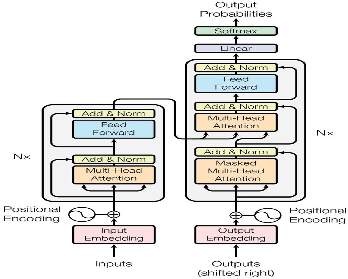
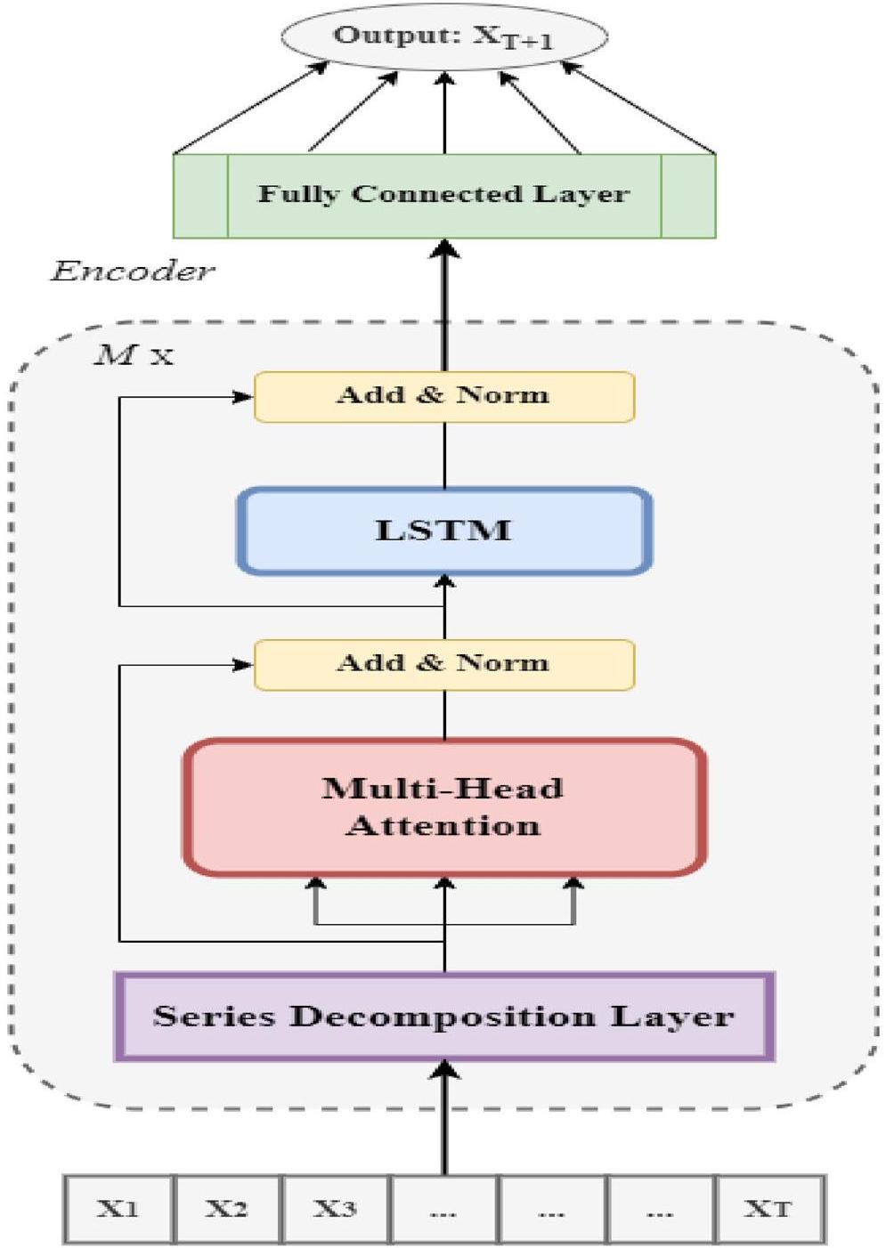
تساعد الاستراتيجية آلية الانتباه على فهم الاتجاهات العالمية بكفاءة. يستخدم نموذج المحول التقليدي ترميز المواقع مقترنًا بتضمين المدخلات لتحويل متجهات الكلمات عالية الأبعاد إلى متجهات منخفضة الأبعاد لتطبيقات معالجة اللغة الطبيعية. تستخدم هذه الدراسة، وهي مشكلة غير متعلقة بمعالجة اللغة الطبيعية، مكون LSTM ليحل محل آلية الشبكة الأمامية (FFN) في الهيكل المشفر لالتقاط الاعتمادات الزمنية، وهي سمة متأصلة في توقعات السلاسل الزمنية. تستخدم هذه العمل فقط مكون التشفير، حيث دعم هاريونو وآخرون [24] الادعاء بأن استخدام مكون تشفير واحد أكثر فعالية من استخدام مكونين مزدوجين، خاصة في توقعات السلاسل الزمنية، لأنه يقلل من تعقيد الذاكرة ومتطلبات الحوسبة.
- تم تصميم نموذج جديد للتنبؤ بالأصول المتقلبة للغاية مثل العملات المشفرة.
- على عكس الدراسات السابقة التي تستخدم بشكل متكرر الضبط اليدوي لنماذج التعلم الآلي، يقوم هذا العمل بتنفيذ تحسين بايزي باستخدام أوبتونا لضبط المعلمات الفائقة لتوليد توقعات قوية.
- تظهر التحليلات التجريبية أخطاءً minimal وأداءً استثنائيًا، متفوقةً على جميع الأساليب والدراسات الحديثة الموجودة.
- هذا العمل هو أول تنفيذ لنموذج هيلفورمر، الذي تم اختبار التحقق منه عبر 15 عملة مشفرة.
- أخيرًا، يعرض هذا العمل الآثار العملية والربحية المحتملة للعملات المشفرة المستهدفة لتوليد عوائد كبيرة.
البحث المتعلق
العملات المشفرة
النهج الكلاسيكي في توقع أسعار العملات المشفرة
ونماذج VAR متعددة المتغيرات للتنبؤ بالنقاط والكثافة، باستخدام متوسط النموذج الديناميكي (DMA) واختيار النموذج الديناميكي (DMS) لدمج هذه النماذج واختيارها. ومن الجدير بالذكر أن شعبية جميع النماذج الكلاسيكية المذكورة أعلاه تنبع من بساطتها وقابليتها للتفسير، ومع ذلك، فإنها غالبًا ما تفشل في التقاط الطبيعة غير الخطية، والطبيعة غير الثابتة، والتعقيدات المعقدة المرتبطة بسوق العملات المشفرة. تحدث هذه القيود بسبب اعتمادها على افتراضات خطية بشأن سلوك السوق. وقد أدى هذا الفجوة إلى اتجاه متزايد نحو استخدام تقنيات أكثر تقدمًا مثل التعلم الآلي التي يمكن أن تتعامل بفعالية مع الطبيعة غير الخطية وغير الثابتة لسوق العملات المشفرة.
نهج التعلم الآلي في توقع أسعار العملات المشفرة
يقدم النموذج نتائج أكثر دقة مقارنة بالنماذج التقليدية مثل Naïve وغيرها. من أجل توقعات قوية، استكشف العديد من الباحثين إمكانية استخدام نماذج التجميع في توقعات العملات المشفرة. على سبيل المثال، قام سون وآخرون [56] بتطبيق آلة تعزيز التدرج الخفيف (LightGBM)، وهي خوارزمية تعلم آلي. وجدت الدراسة أن نموذج LightGBM يتفوق على النماذج التقليدية مثل SVM وRF من حيث القوة ودقة التوقع، خاصة في التوقعات متوسطة المدى (مثل فترات أسبوعين). بعد ذلك، باستخدام تقنيات التعلم الآلي، قام سيباستياو وغودينيو [54] بالتحقيق في إمكانية التنبؤ وربحية استراتيجيات التداول لثلاث عملات مشفرة رئيسية: BTC وETH وLTC. تمتد الدراسة من أغسطس 2015 إلى مارس 2019، وهي فترة تميزت بتقلبات سوقية كبيرة، بما في ذلك الأسواق الصاعدة والهابطة. استخدم المؤلفون نماذج تعلم آلي متعددة، بما في ذلك النماذج الخطية وRF وSVM، لتوقع عوائد العملات المشفرة بناءً على بيانات النشاط التجاري والشبكي. تكشف النتائج أنه على الرغم من أن أداء النماذج الفردية يمكن أن يختلف تحت ظروف السوق المتغيرة، إلا أن نماذج التجميع، وخاصة تلك التي تتطلب توافقًا، تظهر ربحية قوية.
نهج التعلم العميق في توقع أسعار العملات المشفرة
و Bi-LSTM، للتنبؤ بأسعار العملات المشفرة مثل BTC و ETH و LTC. وجدت الدراسة أن نموذج GRU يوفر التنبؤات الأكثر دقة مع أقل خطأ. تم تحقيق نتائج مماثلة في تجربة مماثلة أجراها دوتا وآخرون [15]، هانسون وآخرون [23]، وجين ولي [28]. في المقابل، أعاد سيابي وآخرون [53] تجربة مماثلة مع نتيجة معاكسة حيث تفوق Bi-LSTM على نموذج GRU. مؤخرًا، قدم غولناري وآخرون [19] نهجًا جديدًا في التعلم العميق لتنبؤ أسعار العملات المشفرة، مع التركيز بشكل خاص على BTC. يقترح المؤلفون نموذج GRU الاحتمالي (P-GRU) الذي يدمج ميزات احتمالية لتوفير توزيع احتمالي للقيم المتوقعة، مما يحسن دقة التنبؤ في ظل ظروف السوق المتقلبة. تم مقارنة أداء النموذج مع نماذج أخرى معروفة، بما في ذلك GRU و LSTM ونسخها الاحتمالية، باستخدام بيانات أسعار BTC لمدة عام واحد تم أخذ عينات منها في
الاتجاهات، تحقيق معدلات دقة أعلى. تشمل الدراسات الملحوظة الأخرى التي تظهر دمج الشبكات العصبية التلافيفية في نماذجها الهجينة ليفيريس وآخرون [37]، وزانغ وآخرون [62]، وبنغ وآخرون [47]
نهج قائم على الانتباه لتوقع أسعار العملات المشفرة
الطريقة
Helformer
المكون الموسمي كمتوسط مرجح لنقطة زمنية مستقبلية (
في المستقبل، يتم إضافة طبقات الجمع والتطبيع لأنها حاسمة في استقرار عملية التدريب وتحسين أداء النموذج. إن دمج طبقة الجمع والتطبيع في نموذج هيلفورمر يحسن بشكل كبير من الاستقرار والسرعة في
بيانات
جمع البيانات
| رقم التسلسل | العملة المشفرة | عملات | عينات | تاريخ البدء (يوم/شهر/سنة) | تاريخ الانتهاء (يوم/شهر/سنة) | معنى | الانحراف المعياري |
| 1 | بيتكوين | بيتكوين | ٢٧٣٨ | 01/01/2017 | 30/06/2024 | ٢١,٩٠٨.٩٤ | 18,749.32 |
| 2 | إيثيريوم | إيث | 2426 | 09/11/2017 | 30/06/2024 | ١٣٨١.٢٨ | ١١٩٥.١٨ |
| ٣ | عملة بينانس | بي ان بي | 2426 | 09/11/2017 | 30/06/2024 | ١٩٠.٩٩ | 191.57 |
| ٤ | سولانا | سول | 1543 | 10/04/2020 | 30/06/2024 | ٥٦.٢٩ | 60.04 |
| ٥ | تموج | إكس آر بي | 2426 | 09/11/2017 | 30/06/2024 | 0.52 | 0.32 |
| ٦ | تونكوين | طن | ١٠٣٩ | 27/08/2021 | 30/06/2024 | 2.35 | 1.50 |
| ٧ | دوغ كوين | دوغ | 2426 | 09/11/2017 | 30/06/2024 | 0.06 | 0.08 |
| ٨ | كاردانو | أدا | 2426 | 09/11/2017 | 30/06/2024 | 0.47 | 0.55 |
| 9 | ترون | تي آر إكس | 2426 | 09/11/2017 | 30/06/2024 | 0.05 | 0.03 |
| 10 | انهيار ثلجي | أفاكس | 1380 | 13/07/2020 | 30/06/2024 | 31.50 | ٢٦.٦٣ |
| 11 | شيبا إينو | شيبا | 1171 | 17/04/2021 | 30/06/2024 | 0.00002 | 0.00001 |
| 12 | بولكادوت | نقطة | 1411 | 20/08/2020 | 30/06/2024 | ١٣.٣٥ | 11.49 |
| ١٣ | تشينلينك | رابط | 2426 | 09/11/2017 | 30/06/2024 | 9.46 | 9.44 |
| 14 | بيتكوين كاش | بي سي إتش | 2426 | 09/11/2017 | 30/06/2024 | 427.86 | ٤٠٩.١٨ |
| 15 | واحد لكن أسد | ليو | 1868 | 21/05/2019 | 30/06/2024 | 3.06 | 1.64 |
| 16 | بروتوكول NEAR | قريب | 1356 | 14/10/2020 | 30/06/2024 | ٤.٦٤ | 3.82 |
معالجة البيانات
الإعداد التجريبي
تدمج هذه الدالة السلسة وغير الأحادية Mish خاصية التحكم الذاتي، مشابهة لدالة Swish، مما يسمح لكل خلية عصبية بضبط مخرجاتها بناءً على المدخلات التي تتلقاها. تضمن سلاسة “Mish” وجود مشتقات مستمرة، وهو أمر حاسم للحفاظ على تدفق التدرجات الثابت عبر الشبكات العميقة. يمكن أن يكون هذا مفيدًا بشكل خاص في منع مشكلات مثل انقطاع التدرجات أثناء عملية التعلم. تقدم Mish العديد من الفوائد مقارنةً بوظائف التنشيط التقليدية مثل ReLU وSwish، خاصة في قدرتها على التخفيف من “مشكلة ReLU الميت” من خلال تجنب مناطق التدرجات الصفرية [39]. على عكس ReLU، تسمح Mish بانتشار القيم السلبية، مما يساعد على التقاط المزيد من
| النماذج | Helformer | Transformer | RNN/LSTM/ BiLSTM/ GRU |
| عدد كتل المحول | 1 | 1 | – |
| عدد الرؤوس | 4 | 4 | – |
| حجم الرأس | 16 | 16 | – |
| الانخفاض | 0.1 | 0.1 | 0.1 |
| العصور | 100 | 100 | 100 |
| حجم الدفعة | 32 | 32 | 32 |
| الخلايا العصبية | 30 | – | 30 |
| الطبقات المخفية | – | – | 1 |
| معدل التعلم | 0.001 | 0.001 | 0.001 |
| المحسن | Adams | Adams | Adams |
| الخسارة | MSE | MSE | MSE |
| ff_dim | – | 16 | – |
| دالة التنشيط | Mish | Mish | Mish |
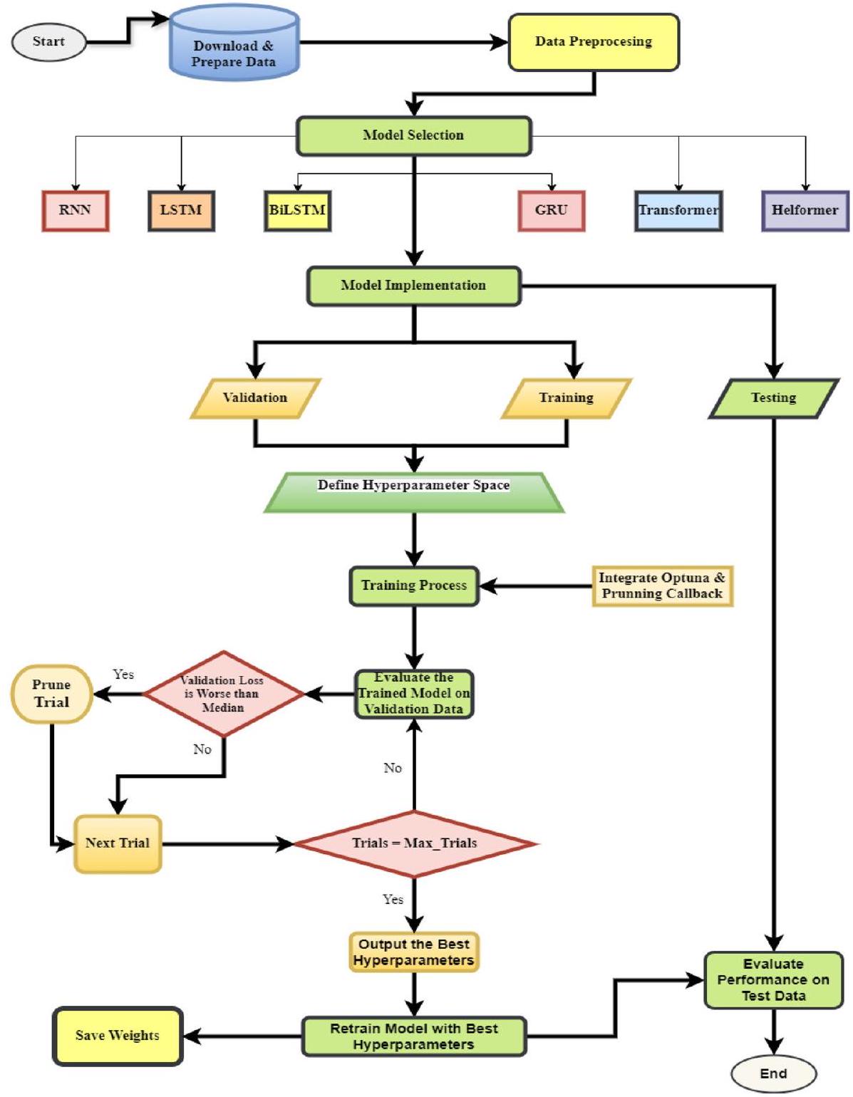
عملية تحسين المعلمات الفائقة
في تحسين بايزي، تُعتبر دالة الهدف
العنصرين: الدالة السابقة والدالة اللاحقة، والتي يتم تمثيلها عادةً بواسطة دالة اكتساب. تقوم الدالة السابقة بنمذجة السلوك المتوقع لدالة الهدف وغالبًا ما يتم تقديرها باستخدام طرق مثل العمليات الغاوسية (GP) أو خوارزميات أكثر تخصصًا مثل مُقدّر بارزين الشجري (TPE) [22]. مع جمع تقييمات الدالة، يتم تحديث السابقة لتشكيل توزيع لاحق، والذي يلتقط رؤى من بيانات جديدة ويقوم بتحسين فهم سلوك الدالة. يعتبر هذا التوزيع اللاحق ضروريًا لبناء دالة اكتساب
- تحديد فضاء البحث: يتم تحقيق ذلك من خلال تحديد القيم الممكنة لكل معلمة فائقة (مثل، معدل التعلم، معدل التسرب، حجم الدفعة).
- تهيئة التجارب العشوائية: يقوم الخوارزمية أولاً بتقييم بعض التكوينات المختارة عشوائيًا لبناء نموذج أولي.
- بناء نموذج بديل: يتم إنشاء نموذج احتمالي لتقريب الدالة الهدف.
- اختيار مجموعة المعلمات الفائقة التالية: بناءً على معيار EI، يتم اختيار المعلمات الفائقة الواعدة التالية.
- تقييم وتحديث النموذج: يتم اختبار مجموعة المعلمات الفائقة الجديدة، ويتم تحديث النموذج البديل بشكل تكراري.
- التقارب: تتوقف العملية عندما تصبح مكاسب الأداء ضئيلة أو عندما يتم الوصول إلى عدد محدد من التجارب.
مقاييس التقييم
| المعلمات الفائقة | RNN/LSTM/BiLSTM/GRU | Transformer | Helformer |
| الخلايا العصبية | [20، 50] (خطوة = 5) | – | [20، 50] (خطوة = 5) |
| الطبقات | [1، 2] | – | – |
| عدد الكتل | – | [1،4] | [1،4] |
| معدل التعلم | [0.0001، 0.01] | [0.0001، 0.01] | [0.0001، 0.01] |
| معدل التسرب | [0، 0.3] | [0،0.3] | [0،0.3] |
| حجم الدفعة | [16، 32، 64، 128] | [16، 32، 64، 128] | [16، 32، 64، 128] |
| عدد الدورات | [50، 150] (خطوة
|
[50، 150] (خطوة = 5) | [50، 150] (خطوة = 5) |
| عدد الرؤوس | – | [2، 10] (خطوة = 2) | [2، 10] (خطوة = 2) |
| حجم الرأس | – | [8، 64] (خطوة = 8) | [8، 64] (خطوة = 8) |
| ff_dim | – | [16، 64] (خطوة = 16) | – |
النتائج التجريبية والمناقشات
نتائج النماذج الأساسية
| نموذج | جذر متوسط مربع الخطأ | ماب | ماي |
|
EVS | KGE |
| شبكة عصبية متكررة | ١٢٥٦.٣٧٦٧ | ٢.٣٩٤٢٪ | 915.7597 | 0.9941 | 0.9952 | 0.9851 |
| LSTM | ١٤٢٦.٥٤٥٣ | ٣.١١٢١٪ | ١١٢٣.٤٢٤٨ | 0.9924 | 0.9930 | 0.9669 |
| بي إل إس تي إم | ١٣٣١.٣٠٤٧ | ٢.٦٠٣٠٪ | 980.5543 | 0.9933 | 0.9937 | 0.9862 |
| GRU | 1314.9097 | ١.٩٢٤١٪ | 830.1504 | 0.9935 | 0.9944 | 0.9674 |
| محول | ١٦٥٧.١٤٢٦ | ٣.٠٠٥٣٪ | 1174.7753 | 0.9897 | 0.9900 | 0.9855 |
| هيلفورمر | ١٦٫٠٨٢٢ | 0.0343% | 13.4487 | 1 | 1 | 0.9995 |
نتائج النماذج المحسّنة
عدد دورات التدريب المحسّنة عند
| نموذج | جذر متوسط مربع الخطأ | ماب | ماي |
|
EVS | KGE |
| شبكة عصبية متكررة | ١١٥٣.١٨٧٧ | ١.٩١٢٢٪ | 765.7482 | 0.9950 | 0.9951 | 0.9905 |
| LSTM | 1171.6701 | 1.7681% | 737.1088 | 0.9948 | 0.9949 | 0.9815 |
| بي إل إس تي إم | 1140.4627 | 1.9514% | ٧٦٦٫٧٢٣٤ | 0.9951 | 0.9952 | 0.9901 |
| GRU | ١١٥١.١٦٥٣ | ١.٧٥٠٠٪ | ٧٢٤.٥٢٧٩ | 0.9950 | 0.9950 | 0.9878 |
| محول | 1218.5600 | ١.٩٦٣١٪ | 799.6003 | 0.9944 | 0.9946 | 0.9902 |
| هيلفورمر | 7.7534 | 0.0148% | 5.9252 | 1 | 1 | 0.9998 |
تنفيذ استراتيجية التداول
| النماذج | العائد الزائد (ER) | التقلب (V) | أقصى انخفاض (MDD) | نسبة شارب (SR) |
| RNN | 157.57% | 0.0246 | -0.1871 | 2.2146 |
| LSTM | 90.88% | 0.0247 | -0.1617 | 1.2611 |
| BiLSTM | 171.23% | 0.0246 | -0.1507 | 2.4117 |
| GRU | 84.76% | 0.0248 | -0.2061 | 1.1743 |
| Transformer | 47.62% | 0.0248 | -0.4369 | 0.6488 |
| Helformer | 925.29% | 0.0178 |
|
18.0604 |
| B&H | 277.01% | 0.0247 | -0.1477 | 1.8529 |
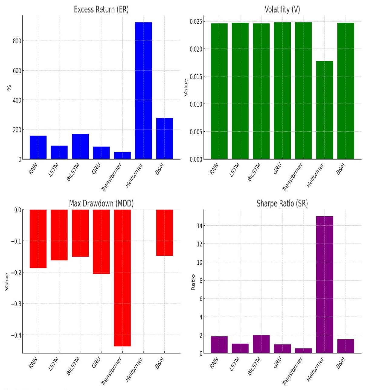
أقصى انخفاض هو مؤشر خطر يحدد أكبر انخفاض في قيمة محفظة أو استثمار من أعلى نقطة إلى أدنى نقطة قبل الوصول إلى ارتفاع جديد. يُستخدم بشكل متكرر لتقييم المخاطر المرتبطة باستثمار معين أو لمقارنة مستويات مخاطر الأصول المختلفة. تُستخدم المعادلة 23 عادةً في حساب أقصى انخفاض.
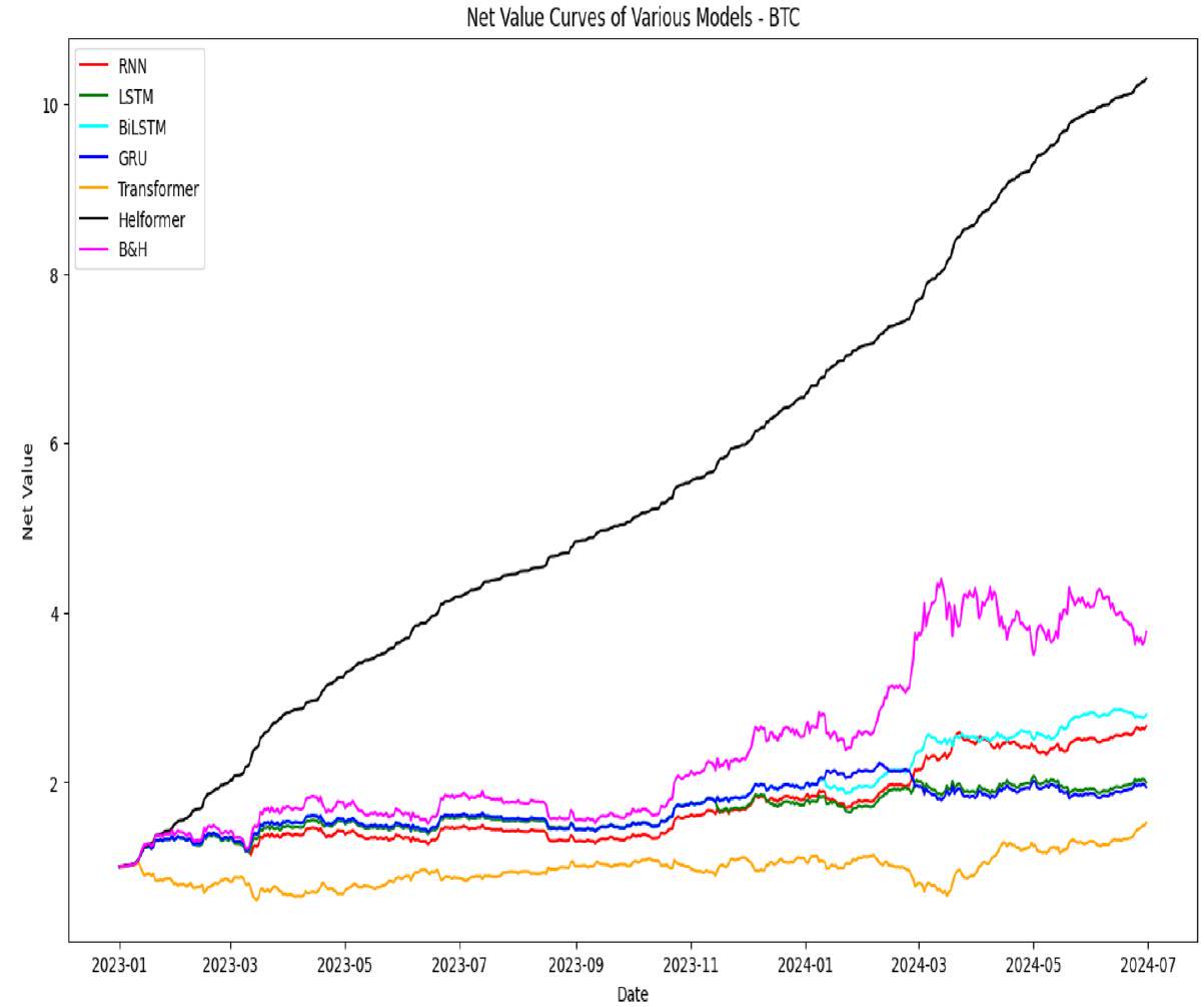
يوضح الجدول 6 فعالية النماذج المختلفة في سياق التداول من خلال إظهار قدرتها على تعظيم العوائد مع تقليل المخاطر. من بين جميع النماذج، يبرز نموذج هيلفورمر بشكل ملحوظ، محققًا ER بنسبة 925.29%. هذا العائد أعلى بكثير من أي نموذج آخر، مما يدل على قدرة هيلفورمر الاستثنائية على تحقيق الربح في سوق العملات المشفرة المتقلبة. بالإضافة إلى ذلك، يُظهر هيلفورمر أقل V بنسبة 0.0178، مما يشير إلى أنه يحافظ على أداء مستقر نسبيًا. MDD لنموذج هيلفورمر يكاد يكون غير ملحوظ عند
منخفض نسبيًا عند -0.1507، ونسبة شارب هي 2.0039، مما يشير إلى توازن جيد بين العائد والمخاطر. ومع ذلك، لا يزال أداؤه بعيدًا عن أداء نموذج هيلفورمر.
مقارنة بين هيلفورمر والدراسات الحالية
المعلمات كما هو موضح في الدراسات المختارة لتوفير مقارنة مباشرة وغير متحيزة. تشمل الدراسات المختارة لهذا التحليل المقارن مجموعة متنوعة من النماذج: النماذج الفردية، النماذج الهجينة، ونماذج التجميع، والتي تمثل بعض من أكثر الأساليب فعالية في أبحاث العملات المشفرة الحديثة. تشمل هذه الأعمال البارزة هانسون وآخرون [23]، سيابي وآخرون [53]، جين ولي [28]، وفلاح وآخرون [16]، الذين استخدموا تقنيات متطورة متنوعة لتعزيز دقة التنبؤ واستراتيجيات التداول. من خلال مقارنة هيلفورمر مع هذه المنهجيات المتنوعة والمتقدمة، تهدف هذه الدراسة إلى تسليط الضوء على قدراته المتفوقة من حيث دقة التنبؤ، والصلابة عبر ظروف السوق المختلفة، وقدرة التعميم عبر عدة عملات مشفرة. تعزز هذه المقارنة الشاملة المقدمة في الجدول 7 من موقف هيلفورمر كنموذج متعدد الاستخدامات وموثوق لتوقع أسعار العملات المشفرة، القادر على التفوق على كل من النماذج التقليدية والنماذج المتطورة المقدمة في الأدبيات الحالية.
| رقم السلسلة | نماذج | جذر متوسط مربع الخطأ | ماب | ماي |
| فلاح وآخرون [16] | ||||
| 1 | أريما | 13,178.34 | ٣٨.٢٠٪ | 11,654.64 |
| 2 | SVR | ١٠٤٣.٩٥ | ٣.٠٠٠٪ | ٨١٨.٤٧ |
| ٣ | RF | ١٠٣٨.٠٨ | ٣.٠٠٪ | ٧٣١.٧٢ |
| ٤ | DNN | 784.42 | 2.10% | 588.16 |
| ٥ | DNN + VAR | 711.40 | 1.80% | ٥٠٨.٤٩ |
| ٦ | هيلفورمر | ٣٦.٢٣ | 0.10% | ٢٧.٨٦ |
| جين ولي [28] | ||||
| 1 | أريما | 253.051 | 1.61% | 172.681 |
| ٢ | RF | ٣٧٢.٧٧٣ | 2.78% | ٢٨٣٫٢٤٦ |
| ٣ | SVM | ٣٣٠.٣٨٩ | 2.23% | 236.284 |
| ٤ | مخبر | ٣٣٣.١٢٤ | ٢.٤٨٪ | 257.918 |
| ٥ | أوتوفورمر | ٤٠٢.١٩٦ | 3.08% | ٣١٩.٢٥٧ |
| ٦ | LSTM | ٢٧٥.٩٥٨ | 1.82% | 193.817 |
| ٧ | GRU | 260.502 | 1.69% | ١٨٠.٥٠١ |
| ٨ | EMD-AGRU-LSTM | ٢٢٣.٥٥٦ | 1.75% | 181.721 |
| 9 | VMD-AGRU-GRU | 150.032 | 1.04% | ١١٣.٣٢ |
| 10 | VMD-GRU-LSTM | 127.284 | 0.88% | 94.895 |
| 11 | VMD-AGRU-LSTM | ١٢٤.٦٥٧ | 0.87% | 93.756 |
| 12 | VMD-AGRU-RESEMD-LSTM | ١٠٥.١٣ | 0.75% | 80.417 |
| ١٣ | VMD-AGRU-RESVMD-LSTM | 50.651 | 0.39% | 42.298 |
| 14 | هيلفورمر | 0.201 | 0.0014% | 0.153 |
| سيبي وآخرون [53] | ||||
| 1 | LSTM | ١٠٣١.٣٤٠١ | 3.94% | – |
| 2 | بي إل إس تي إم | ١٠٢٩.٣٦١٧ | 3.56% | – |
| ٣ | GRU | 1274.1706 | 5.72% | – |
| ٤ | هيلفورمر | 19.7973 | 0.050% | |
| هانسون وآخرون [23] | ||||
| 1 | LSTM | ٢٥١٨.٠٢١٧ | ٤.٢١٨٪ | 1617.7592 |
| 2 | بي إل إس تي إم | ٢٢٢٢.٧٣٥٤ | ٣.٨٠٠٪ | ١٤٢٢.١٩٣٣ |
| ٣ | GRU | 1777.306 | ٣.٤٩٢٪ | ١١٦٧.٣٤٦١ |
| ٤ | هيلفورمر | 8.0665 | 0.010% | ٣.٧٦٧٠ |
قدرة هيلفورمر على التعميم والتعلم الانتقالي
| رقم التسلسل | العملة المشفرة | جذر متوسط مربع الخطأ | ماب | ماي |
|
EVS | KGE |
| 1 | إيث | 15.0676 | 0.6039% | 14.0754 | 0.9995 | 0.9999 | 0.9916 |
| 2 | بي ان بي | 9.2982 | ٢.٤٦٢٩٪ | 8.5706 | 0.9957 | 0.9993 | 0.9652 |
| ٣ | سول | 2.6935 | ٢.٣٣١١٪ | ٢.٣٤٤٧ | 0.9976 | 0.9994 | 0.9670 |
| ٤ | إكس آر بي | 0.0014 | 0.2644% | 0.0014 | 0.9996 | 0.9999 | 0.9962 |
| ٥ | طن | 0.0085 |
|
0.0076 | 0.9999 | 1 | 0.9974 |
| ٦ | دوغ | 0.0001 | 0.0606% |
|
0.9999 | 0.9999 | 0.9998 |
| ٧ | أدا | 0.0020 | 0.4564% | 0.0018 | 0.9997 | 0.9999 | 0.9935 |
| ٨ | تي آر إكس |
|
|
|
1 | 1 | 1 |
| 9 | أفاكس | 0.4701 | 1.3067% | 0.4270 | 0.9986 | 0.9997 | 0.9813 |
| 10 | شيبا |
|
٢.٤٦٢٣٪ |
|
0.9966 | 0.9993 | 0.9653 |
| 11 | نقطة | 0.1339 | ١.٨٥١٠٪ | 0.1258 | 0.9939 | 0.9992 | 0.9738 |
| 12 | رابط | 0.3891 | ٣.٠٤٤٧٪ | 0.3510 | 0.9936 | 0.9988 | 0.9570 |
| ١٣ | بي سي إتش | 10.0356 | ٣.٢٤٩٤٪ | 8.7577 | 0.9944 | 0.9986 | 0.9541 |
| 14 | ليو | 0.1465 | ٣.١٢٦٨٪ | 0.1424 | 0.9742 | 0.9985 | 0.9558 |
| 15 | قريب | 0.0461 | 0.8978% | 0.0385 | 0.9995 | 0.9998 | 0.9876 |
| رقم التسلسل | استراتيجية تداول العملات | هيلفورمر | بي آند إتش | ||||||
| نسبة الطوارئ (%) | ف | اضطراب الاكتئاب الشديد | ريال سعودي | نسبة الطوارئ (%) | ف | اضطراب الاكتئاب الشديد | ريال سعودي | ||
| 1 | إيث | 854.88 | 0.0204 | -0.0043 | 16.46 | ١١٩.٠٨ | 0.0272 | -0.2456 | 1.12 |
| 2 | بي ان بي | ٤٩٣.٨٠ | 0.0244 | -0.0502 | ٧.٩٥ | 100.95 | 0.0266 | -0.4462 | 1.01 |
| ٣ | شمس | 937.72 | 0.0371 | -0.0358 | 15.70 | 612.61 | 0.0481 | -0.1940 | 2.52 |
| ٤ | إكس آر بي | ١٠٤٤.١٨ | 0.0331 | -0.0007 | 12.41 | ٢٧.١٩ | 0.0399 | -0.3125 | 0.22 |
| ٥ | طن | 668.86 | 0.0320 | -0.0010 | 19.36 | 236.66 | 0.0456 | -0.1826 | 2.45 |
| ٦ | دوغ | ١٣٥٤.٧٩ | 0.0305 | -0.0004 | 17.51 | 66.72 | 0.0418 | -0.4040 | 0.47 |
| ٧ | أدا | ١٢٠٤.٥٢ | 0.0250 | -0.0017 | 18.93 | ١٦.٥٥ | 0.0356 | -0.4839 | 0.15 |
| ٨ | تي آر إكس | 656.68 | 0.0148 | 0.0000 | 17.42 | ٨٦.٧٤ | 0.0202 | -0.1586 | 1.19 |
| 9 | أفاكس | ٩٨٨٫٩٤ | 0.0352 | -0.0061 | 19.45 | ٢١٩.٩٩ | 0.0507 | -0.3093 | 1.58 |
| 10 | شيبا | ٨٣١.٦٦ | 0.0555 | 0.0000 | 12.26 | ٨٨.٨٨ | 0.0666 | -0.3144 | 0.77 |
| 11 | نقطة | ٦٩٢.٤٢ | 0.0310 | -0.0252 | 15.14 | 53.96 | 0.0399 | -0.3515 | 0.72 |
| 12 | رابط | ٨٨٢.٦٣ | 0.0345 | -0.0350 | 10.05 | ١٠٨.١٠ | 0.0394 | -0.4214 | 0.72 |
| ١٣ | بي سي إتش | 846.55 | 0.0437 | -0.0411 | 7.62 | 216.39 | 0.0474 | -0.2667 | 0.94 |
| 14 | ليو | 167.04 | 0.0169 | -0.0654 | ٥.٠٢ | ٤٨.٥٣ | 0.0176 | -0.1247 | 1.12 |
| 15 | قريب | ١١٥٩.٣٩ | 0.0434 | -0.0079 | 18.87 | ٣٨٢.٣٤ | 0.0614 | -0.2062 | 1.80 |
الخاتمة، القيود، والاتجاهات المستقبلية
استراتيجيات التحسين، يتعامل نموذج هيلفورمر مع الطبيعة المتقلبة للعملات المشفرة، مما يتيح مجالاً لاستراتيجيات استثمار أكثر استقرارًا وقابلية للتنبؤ.
الشكر والتقدير
مساهمات المؤلفين
التمويل
توفر البيانات والمواد
الإعلانات
موافقة الأخلاقيات والموافقة على المشاركة
المصالح المتنافسة
تاريخ الاستلام: 15 ديسمبر 2024 تاريخ القبول: 25 مارس 2025
تاريخ النشر على الإنترنت: 03 أبريل 2025
References
- Abu Bakar N, Rosbi S. Autoregressive integrated moving average (ARIMA) model for forecasting cryptocurrency exchange rate in high volatility environment: a new insight of bitcoin transaction. Int J Adv Eng Res Sci. 2017;4(11):130-7.
- Akyildirim E, Goncu A, Sensoy A. Prediction of cryptocurrency returns using machine learning. Ann Oper Res. 2021;297:3-36.
- Alonso-Monsalve S, Suárez-Cetrulo AL, Cervantes A, Quintana D. Convolution on neural networks for high-frequency trend prediction of cryptocurrency exchange rates using technical indicators. Expert Syst Appl. 2020;149: 113250.
- Amadeo, A. J., Siento, J. G., Eikwine, T. A., & Parmonangan, I. H. Temporal Fusion Transformer for Multi Horizon Bitcoin Price Forecasting. 2023 IEEE 9th Information Technology International Seminar (ITIS), 2023
- Beltagy, I., Peters, M. E., & Cohan, A. (2020). Longformer: The long-document transformer. arXiv preprint arXiv:2004. 05150.
- Bergstra J, Bengio Y. Random search for hyper-parameter optimization. J Mach Learn Res. 2012;13(2):2.
- Bouteska A, Abedin MZ, Hajek P, Yuan K. Cryptocurrency price forecasting-a comparative analysis of ensemble learning and deep learning methods. Int Rev Financ Anal. 2024;92: 103055.
- Catania L, Grassi S, Ravazzolo F. Forecasting cryptocurrencies under model and parameter instability. Int J Forecast. 2019;35(2):485-501.
- Cavalli S, Amoretti M. CNN-based multivariate data analysis for bitcoin trend prediction. Appl Soft Comput. 2021;101: 107065.
- Chang T-J, Lee T-S, Yang C-T, Lu C-J. A ternary-frequency cryptocurrency price prediction scheme by ensemble of clustering and reconstructing intrinsic mode functions based on CEEMDAN. Expert Syst Appl. 2023;233: 121008.
- Chowdhury R, Rahman MA, Rahman MS, Mahdy M. An approach to predict and forecast the price of constituents and index of cryptocurrency using machine learning. Physica A. 2020;551: 124569.
- Conrad C, Custovic A, Ghysels E. Long-and short-term cryptocurrency volatility components: a GARCH-MIDAS analysis. J Risk Financ Manag. 2018;11(2):23.
- Da Silva, R. G., Ribeiro, M. H. D. M., Fraccanabbia, N., Mariani, V. C., & dos Santos Coelho, L. Multi-step ahead bitcoin price forecasting based on VMD and ensemble learning methods. 2020 International Joint Conference on Neural Networks (IJCNN). 2020
- Du X, Tang Z, Wu J, Chen K, Cai Y. A new hybrid cryptocurrency returns forecasting method based on multiscale decomposition and an optimized extreme learning machine using the sparrow search algorithm. leee Access. 2022;10:60397-411.
- Dutta A, Kumar S, Basu M. A gated recurrent unit approach to bitcoin price prediction. J Risk Financ Manag. 2020;13(2):23.
- Fallah MF, Pourmansouri R, Ahmadpour B. Presenting a new deep learning-based method with the incorporation of error effects to predict certain cryptocurrencies. Int Rev Financ Anal. 2024;95: 103466.
- Ghosh I, Jana RK, Sharma DK. A novel granular decomposition based predictive modeling framework for cryptocurrencies’ prices forecasting. China Financ Rev Int. 2024. https://doi.org/10.1108/CFRI-03-2023-0072.
- Girsang AS. Hybrid LSTM and GRU for cryptocurrency price forecasting based on social network sentiment analysis using FinBERT. leee Access. 2023;11:120530-40.
- Golnari A, Komeili MH, Azizi Z. Probabilistic deep learning and transfer learning for robust cryptocurrency price prediction. Expert Syst Appl. 2024. https://doi.org/10.1016/j.eswa.2024.124404.
- Goodell JW, Jabeur SB, Saâdaoui F, Nasir MA. Explainable artificial intelligence modeling to forecast bitcoin prices. Int Rev Financ Anal. 2023;88: 102702.
- Hamayel MJ, Owda AY. A novel cryptocurrency price prediction model using GRU, LSTM and bi-LSTM machine learning algorithms. Ai. 2021;2(4):477-96.
- Hanifi S, Cammarono A, Zare-Behtash H. Advanced hyperparameter optimization of deep learning models for wind power prediction. Renew Energy. 2024;221: 119700.
- Hansun S, Wicaksana A, Khaliq AQ. Multivariate cryptocurrency prediction: comparative analysis of three recurrent neural networks approaches. J Big Data. 2022;9(1):50.
- Haryono AT, Sarno R, Sungkono KR. Transformer-gated recurrent unit method for predicting stock price based on news sentiments and technical indicators. leee Access. 2023. https://doi.org/10.1109/ACCESS.2023.3298445.
- Ho K-H, Hou Y, Georgiades M, Fong KC. Exploring key properties and predicting price movements of cryptocurrency market using social network analysis. leee Access. 2024. https://doi.org/10.1109/ACCESS.2024.3397723.
- Ibrahim A, Kashef R, Corrigan L. Predicting market movement direction for bitcoin: A comparison of time series modeling methods. Comput Electr Eng. 2021;89: 106905.
- Jay P, Kalariya V, Parmar P, Tanwar S, Kumar N, Alazab M. Stochastic neural networks for cryptocurrency price prediction. leee Access. 2020;8:82804-18.
- Jin C, Li Y. Cryptocurrency price prediction using frequency decomposition and deep learning. Fractal Fract. 2023;7(10):708.
- Kehinde T, Chan FT, Chung S. Scientometric review and analysis of recent approaches to stock market forecasting: two decades survey. Expert Syst Appl. 2023;213: 119299.
- Kehinde T, Chung S, Chan FT. Benchmarking TPU and GPU for Stock Price Forecasting Using LSTM Model Development. In: Science and information conference. Cham: Springer; 2023.
- Koo E, Kim G. Centralized decomposition approach in LSTM for Bitcoin price prediction. Expert Syst Appl. 2024;237: 121401.
- Kristjanpoller W, Minutolo MC. A hybrid volatility forecasting framework integrating GARCH, artificial neural network, technical analysis and principal components analysis. Expert Syst Appl. 2018;109:1-11.
- Kumarappan J, Rajasekar E, Vairavasundaram S, Kotecha K, Kulkarni A. Siamese graph convolutional split-attention network with NLP based social sentimental data for enhanced stock price predictions. J Big Data. 2024;11(1):154.
- Li J, Zhang Y, Yang X, Chen L. Online portfolio management via deep reinforcement learning with high-frequency data. Inf Process Manage. 2023;60(3): 103247.
- Li Y, Jiang S, Li X, Wang S. Hybrid data decomposition-based deep learning for bitcoin prediction and algorithm trading. Financ Innov. 2022;8(1):31.
- Liu M, Li G, Li J, Zhu X, Yao Y. Forecasting the price of Bitcoin using deep learning. Financ Res Lett. 2021;40: 101755.
- Livieris IE, Kiriakidou N, Stavroyiannis S, Pintelas P. An advanced CNN-LSTM model for cryptocurrency forecasting. Electronics. 2021;10(3):287.
- Lu, Y., Zhang, H., & Guo, Q. (2023). Stock and market index prediction using Informer network. arXiv preprint arXiv: 2305.14382.
- Misra, D. (2019). Mish: A self regularized non-monotonic activation function. arXiv preprint arXiv:1908.08681.
- Nakamoto, S. (2008). Bitcoin: A peer-to-peer electronic cash system. Satoshi Nakamoto.
- Nakano M, Takahashi A, Takahashi S. Bitcoin technical trading with artificial neural network. Physica A. 2018;510:587-609.
- Nasirtafreshi I. Forecasting cryptocurrency prices using recurrent neural network and long short-term memory. Data Knowl Eng. 2022;139: 102009.
- Otabek S, Choi J. From prediction to profit: a comprehensive review of cryptocurrency trading strategies and price forecasting techniques. leee Access. 2024. https://doi.org/10.1109/ACCESS.2024.3417449.
- Oyedele AA, Ajayi AO, Oyedele LO, Bello SA, Jimoh KO. Performance evaluation of deep learning and boosted trees for cryptocurrency closing price prediction. Expert Syst Appl. 2023;213: 119233.
- Oyewola DO, Dada EG, Ndunagu JN. A novel hybrid walk-forward ensemble optimization for time series cryptocurrency prediction. Heliyon. 2022. https://doi.org/10.1016/j.heliyon.2022.e11862.
- Patel MM, Tanwar S, Gupta R, Kumar N. A deep learning-based cryptocurrency price prediction scheme for financial institutions. J Inf Security Appl. 2020;55: 102583.
- Peng P, Chen Y, Lin W, Wang JZ. Attention-based CNN-LSTM for high-frequency multiple cryptocurrency trend prediction. Expert Syst Appl. 2024;237: 121520.
- Poongodi M, Nguyen TN, Hamdi M, Cengiz K. Global cryptocurrency trend prediction using social media. Inf Process Manag. 2021;58(6): 102708. https://doi.org/10.1016/j.ipm.2021.102708.
- Quan SJ. Comparing hyperparameter tuning methods in machine learning based urban building energy modeling: a study in Chicago. Energy Build. 2024. https://doi.org/10.1016/j.enbuild.2024.114353.
- Rathore RK, Mishra D, Mehra PS, Pal O, Hashim AS, Shapi’i A, Ciano T, Shutaywi M. Real-world model for bitcoin price prediction. Inf Process Manag. 2022;59(4):102968. https://doi.org/10.1016/j.ipm.2022.102968.
- Saheed YK, Kehinde TO, Ayobami Raji M, Baba UA. Feature selection in intrusion detection systems: a new hybrid fusion of Bat algorithm and Residue Number System. J Inf Telecommun. 2024;8(2):189-207.
- Sbrana A, Lima de Castro PA. N-BEATS perceiver: a novel approach for robust cryptocurrency portfolio forecasting. Comput Econ. 2023;2:1-35.
- Seabe PL, Moutsinga CRB, Pindza E. Forecasting cryptocurrency prices using LSTM, GRU, and bi-directional LSTM: a deep learning approach. Fractal Fract. 2023;7(2):203.
- Sebastião H, Godinho P. Forecasting and trading cryptocurrencies with machine learning under changing market conditions. Financ Innov. 2021;7:1-30.
- Smyl S. A hybrid method of exponential smoothing and recurrent neural networks for time series forecasting. Int J Forecast. 2020;36(1):75-85.
- Sun X, Liu M, Sima Z. A novel cryptocurrency price trend forecasting model based on LightGBM. Financ Res Lett. 2020;32: 101084.
- Tanwar, A., & Kumar, V. (2022). Prediction of cryptocurrency prices using transformers and long short term neural networks. 2022 International Conference on Intelligent Controller and Computing for Smart Power (ICICCSP),
- Touzani Y, Douzi K. An LSTM and GRU based trading strategy adapted to the Moroccan market. J Big Data. 2021;8(1):126.
- Vaswani A, Shazeer N, Parmar N, Uszkoreit J, Jones L, Gomez AN, Kaiser Ł, Polosukhin I. Attention is all you need. Adv Neural Inf Process Syst. 2017;30:1.
- Walther T, Klein T, Bouri E. Exogenous drivers of Bitcoin and Cryptocurrency volatility-a mixed data sampling approach to forecasting. J Int Finan Markets Inst Money. 2019;63: 101133.
- Wu H, Xu J, Wang J, Long M. Autoformer: decomposition transformers with auto-correlation for long-term series forecasting. Adv Neural Inf Process Syst. 2021;34:22419-30.
- Zhang Z, Dai H-N, Zhou J, Mondal SK, García MM, Wang H. Forecasting cryptocurrency price using convolutional neural networks with weighted and attentive memory channels. Expert Syst Appl. 2021;183: 115378.
- Zhong C, Du W, Xu W, Huang Q, Zhao Y, Wang M. LSTM-ReGAT: a network-centric approach for cryptocurrency price trend prediction. Decis Support Syst. 2023;169: 113955.
- Zhou H, Zhang S, Peng J, Zhang S, Li J, Xiong H, Zhang W. Informer: Beyond efficient transformer for long sequence time-series forecasting. Proc AAAI Conf Artif Intell. 2021. https://doi.org/10.1609/aaai.v35i12.17325.
- Zhou T, Ma Z, Wen Q, Wang X, Sun L, Jin R. Fedformer: frequency enhanced decomposed transformer for long-term series forecasting. Int Conf Mach Learn. 2022;162:27268.
- Zhou Z, Song Z, Xiao H, Ren T. Multi-source data driven cryptocurrency price movement prediction and portfolio optimization. Expert Syst Appl. 2023;219: 119600.
- Zoumpekas T, Houstis E, Vavalis M. ETH analysis and predictions utilizing deep learning. Expert Syst Appl. 2020;162: 113866.
ملاحظة الناشر
- © المؤلفون 2025. الوصول المفتوح، هذه المقالة مرخصة بموجب رخصة المشاع الإبداعي للاستخدام غير التجاري، والتي تسمح بأي استخدام غير تجاري، ومشاركة، وتوزيع، وإعادة إنتاج في أي وسيلة أو صيغة، طالما أنك تعطي الائتمان المناسب للمؤلفين الأصليين والمصدر، وتوفر رابطًا لرخصة المشاع الإبداعي، وتوضح إذا قمت بتعديل المادة المرخصة. ليس لديك إذن بموجب هذه الرخصة لمشاركة المواد المعدلة المشتقة من هذه المقالة أو أجزاء منها. الصور أو المواد الأخرى من طرف ثالث في هذه المقالة مشمولة في رخصة المشاع الإبداعي للمقالة، ما لم يُشار إلى خلاف ذلك في سطر ائتمان للمادة. إذا لم تكن المادة مشمولة في رخصة المشاع الإبداعي للمقالة واستخدامك المقصود غير مسموح به بموجب اللوائح القانونية أو يتجاوز الاستخدام المسموح به، ستحتاج إلى الحصول على إذن مباشرة من صاحب حقوق الطبع والنشر. لعرض نسخة من هذه الرخصة، قم بزيارة http://creativecommons.org/licenses/by-nc-nd/4.0/.
DOI: https://doi.org/10.1186/s40537-025-01135-4
Publication Date: 2025-04-03
Helformer: an attention-based deep learning model for cryptocurrency price forecasting
Abstract
Cryptocurrencies have become a significant asset class, attracting considerable attention from investors and researchers due to their potential for high returns despite inherent price volatility. Traditional forecasting methods often fail to accurately predict price movements as they do not account for the non-linear and non-stationary nature of cryptocurrency data. In response to these challenges, this study introduces the Helformer model, a novel deep learning approach that integrates Holt-Winters exponential smoothing with Transformer-based deep learning architecture. This integration allows for a robust decomposition of time series data into level, trend, and seasonality components, enhancing the model’s ability to capture complex patterns in cryptocurrency markets. To optimize the model’s performance, Bayesian hyperparameter tuning via Optuna, including a pruner callback, was utilized to efficiently find optimal model parameters while reducing training time by early termination of suboptimal training runs. Empirical results from testing the Helformer model against other advanced deep learning models across various cryptocurrencies demonstrate its superior predictive accuracy and robustness. The model not only achieves lower prediction errors but also shows remarkable generalization capabilities across different types of cryptocurrencies. Additionally, the practical applicability of the Helformer model is validated through a trading strategy that significantly outperforms traditional strategies, confirming its potential to provide actionable insights for traders and financial analysts. The findings of this study are particularly beneficial for investors, policymakers, and researchers, offering a reliable tool for navigating the complexities of cryptocurrency markets and making informed decisions.
Introduction
as Support Vector Machine (SVM), k-Nearest Neighbors (KNN) [51], and Multi-Level Perceptron (MLP) are non-parametric and do not require a prior understanding of the distribution of data to model the non-linear relationship among variables. However, one of the limitations of using machine learning is that they are susceptible to overfitting, especially when handling long sequence time series forecasting (LSTF) data such as cryptocurrency data. Another limitation is that their models produce a more considerable error, making the model perform poorly when subjected to trading strategy. In this regard, deep learning was later introduced to explore and overcome the weakness of machine learning models.
strategy helps the attention mechanism grasp global trends efficiently. The conventional Transformer model uses positional encoding coupled with input embedding to turn high-dimensional word vectors into low-dimensional ones for NLP applications. This study, a non-NLP problem, uses an LSTM component to substitute a Feed Forward Network (FFN) mechanism in the Encoded architecture to capture temporal dependencies, an attribute inherent in time series forecasting. This work uses only the encoder component, as Haryono et al. [24] supported the claim that using a single encoder component is more effective than using dual components, especially in time series prediction, because it reduces memory complexity and computational demand.
- A novel model is designed to predict highly volatile assets like cryptocurrency.
- Unlike previous studies that frequently use manual tuning for machine learning models, this work implements Bayesian optimization with Optuna for hyperparameter tuning to generate robust predictions.
- Empirical analysis shows minimal errors and exceptional performance, outperforming all existing state-of-the-art methods and studies.
- This work is the first implementation of the Helformer model, the validation of which was tested across 15 cryptocurrencies.
- Last, this work showcases the practical implications and potential profitability of targeted cryptocurrencies to generate substantial returns.
Related research
Cryptocurrency
Classical approach to cryptocurrency price forecasting
and multivariate VAR models for point and density forecasting, utilizing dynamic model averaging (DMA) and dynamic model selection (DMS) to combine and select among these models. Notably, the popularity of all the aforementioned classical models stems from their simplicity and interpretability,however, they frequently fail to capture the non-linear nature, non-stationary nature, and intricate complexities associated with the cryptocurrency market. This limitation occurs due to their dependence on linear assumptions regarding market behaviour. This gap has resulted in an increasing trend towards using more advanced techniques like machine learning that can effectively handle the non-linear and non-stationary nature of the cryptocurrency market.
Machine learning approach to cryptocurrency price forecasting
model yields more accurate results compared to Naïve and other traditional models. For robust predictions, many researchers have explored the possibility of using ensemble models for cryptocurrency forecasting. For instance, Sun et al. [56] apply a Light Gradient Boosting Machine (LightGBM), a machine learning algorithm. The study finds that the LightGBM model outperforms traditional models such as SVM and RF in terms of robustness and forecasting accuracy, particularly in medium-term predictions (e.g., 2-week periods). Next, using machine learning techniques, Sebastião and Godinho [54] investigate the predictability and profitability of trading strategies for three major cryptocurrencies: BTC, ETH, and LTC. The study spans from August 2015 to March 2019, a period marked by significant market fluctuations, including bull and bear markets. The authors employ multiple machine learning models, including linear models, RF, and SVM, to forecast cryptocurrency returns based on trading and network activity data. The findings reveal that although individual models’ performance can vary under changing market conditions, ensemble models, particularly ones requiring consensus, show robust profitability.
Deep learning approach to cryptocurrency price forecasting
and Bi-LSTM, to predict the prices of cryptocurrencies such as BTC, ETH, and LTC. The study finds that the GRU model provides the most accurate predictions with the lowest error. Similar results were achieved in a similar experiment performed by Dutta et al. [15], Hansun et al. [23], and Jin and Li [28]. In contrast, Seabe et al. [53] repeated a similar experiment with a contrary result where Bi-LSTM outperforms the GRU model. More recently, Golnari et al. [19] presented a novel deep learning approach for predicting cryptocurrency prices, focusing specifically on BTC. The authors propose a Probabilistic GRU (P-GRU) model that incorporates probabilistic features to provide a probability distribution for predicted values, improving prediction accuracy under volatile market conditions. The model’s performance was compared with other established models, including GRU, LSTM, and their probabilistic variants, using 1 year of BTC price data sampled at
trends, achieving higher accuracy rates. Other notable studies that demonstrate CNN incorporation in their hybrid models include Livieris et al. [37], Zhang et al. [62], and Peng et al. [47]
Attention-based approach to cryptocurrency price forecasting
Methodology
Helformer
the seasonal component as a weighted mean for a future time point (
Going forward, the add & norm layers are added as they are critical in stabilizing the training process and improving model performance. The incorporation of the add & norm layer in the Helformer model greatly improves stability and speed in
Data
Data collection
| S/N | Cryptocurrency | Coins | Samples | Start date (dd/ mm/yyyy) | End date (dd/ mm/yyyy) | Mean | Std. Dev |
| 1 | BTC | BTC | 2738 | 01/01/2017 | 30/06/2024 | 21,908.94 | 18,749.32 |
| 2 | Ethereum | ETH | 2426 | 09/11/2017 | 30/06/2024 | 1381.28 | 1195.18 |
| 3 | Binance coin | BNB | 2426 | 09/11/2017 | 30/06/2024 | 190.99 | 191.57 |
| 4 | Solana | SOL | 1543 | 10/04/2020 | 30/06/2024 | 56.29 | 60.04 |
| 5 | Ripple | XRP | 2426 | 09/11/2017 | 30/06/2024 | 0.52 | 0.32 |
| 6 | Toncoin | TON | 1039 | 27/08/2021 | 30/06/2024 | 2.35 | 1.50 |
| 7 | Dogecoin | DOGE | 2426 | 09/11/2017 | 30/06/2024 | 0.06 | 0.08 |
| 8 | Cardano | ADA | 2426 | 09/11/2017 | 30/06/2024 | 0.47 | 0.55 |
| 9 | Tron | TRX | 2426 | 09/11/2017 | 30/06/2024 | 0.05 | 0.03 |
| 10 | Avalanche | AVAX | 1380 | 13/07/2020 | 30/06/2024 | 31.50 | 26.63 |
| 11 | Shiba Inu | SHIB | 1171 | 17/04/2021 | 30/06/2024 | 0.00002 | 0.00001 |
| 12 | Polkadot | DOT | 1411 | 20/08/2020 | 30/06/2024 | 13.35 | 11.49 |
| 13 | Chainlink | LINK | 2426 | 09/11/2017 | 30/06/2024 | 9.46 | 9.44 |
| 14 | BTC cash | BCH | 2426 | 09/11/2017 | 30/06/2024 | 427.86 | 409.18 |
| 15 | Unus sed leo | LEO | 1868 | 21/05/2019 | 30/06/2024 | 3.06 | 1.64 |
| 16 | NEAR protocol | NEAR | 1356 | 14/10/2020 | 30/06/2024 | 4.64 | 3.82 |
Data preprocessing
Experimental set-up
This smooth, non-monotonic Mish function integrates a self-gating property, similar to the Swish function, allowing each neuron to adjust its output based on the input it receives. The smoothness of “Mish” ensures continuous derivatives, which are crucial for maintaining a steady gradient flow through deep networks. This can be particularly advantageous in preventing issues like gradient discontinuities during the learning process. Mish offers several benefits over traditional activation functions such as ReLU and Swish, particularly in its ability to mitigate the “dying ReLU problem” by avoiding zero-gradient regions [39]. Unlike ReLU, Mish allows for the propagation of negative values, which helps capture more
| Models | Helformer | Transformer | RNN/LSTM/ BiLSTM/ GRU |
| num_transformer_blocks | 1 | 1 | – |
| num_heads | 4 | 4 | – |
| head_size | 16 | 16 | – |
| dropout | 0.1 | 0.1 | 0.1 |
| epochs | 100 | 100 | 100 |
| batch_size | 32 | 32 | 32 |
| neurons | 30 | – | 30 |
| hidden_layers | – | – | 1 |
| learning_rate | 0.001 | 0.001 | 0.001 |
| optimizer | Adams | Adams | Adams |
| loss | MSE | MSE | MSE |
| ff_dim | – | 16 | – |
| activation function | Mish | Mish | Mish |
Hyperparameters optimization process
In Bayesian optimization, the objective function
elements: the prior function and the posterior function, the latter typically represented by an acquisition function. The prior function models the expected behaviour of the objective function and is often estimated using methods such as Gaussian Processes (GP) or more specialized algorithms like the Tree-structured Parzen Estimator (TPE) [22]. As evaluations of the function are collected, the prior is updated to form a posterior distribution, which captures insights from new data and refines the understanding of the function’s behaviour. This posterior distribution is essential for constructing an acquisition function
- Define the Search Space: This is achieved by specifying the possible values for each hyperparameter (e.g., learning rate, dropout rate, batch size).
- Initialize Random Trials: The algorithm first evaluates a few randomly chosen configurations to build an initial model.
- Build a Surrogate Model: A probabilistic model is constructed to approximate the objective function.
- Select the Next Set of Hyperparameters: Based on the EI criterion, the next promising hyperparameters are selected.
- Evaluate and Update the Model: The new hyperparameter combination is tested, and the surrogate model is updated iteratively.
- Convergence: The process stops when performance gains become negligible or when a set number of trials is reached.
Evaluation metrics
| Hyperparameters | RNN/LSTM/BiLSTM/GRU | Transformer | Helformer |
| neurons | [20, 50] (step = 5) | – | [20, 50] (step = 5) |
| layers | [1, 2] | – | – |
| num_blocks | – | [1,4] | [1,4] |
| learning_rate | [0.0001, 0.01] | [0.0001, 0.01] | [0.0001, 0.01] |
| dropout_rate | [0, 0.3] | [0,0.3] | [0,0.3] |
| batch_size | [16, 32, 64, 128] | [16, 32, 64, 128] | [16, 32, 64, 128] |
| epochs | [50, 150] (step
|
[50, 150] (step = 5) | [50, 150] (step = 5) |
| num_heads | – | [2, 10] (step = 2) | [2, 10] (step = 2) |
| head_size | – | [8, 64] (step = 8) | [8, 64] (step = 8) |
| ff_dim | – | [16, 64] (step = 16) | – |
Empirical results and discussions
Results of the base models
| Model | RMSE | MAPE | MAE |
|
EVS | KGE |
| RNN | 1256.3767 | 2.3942% | 915.7597 | 0.9941 | 0.9952 | 0.9851 |
| LSTM | 1426.5453 | 3.1121% | 1123.4248 | 0.9924 | 0.9930 | 0.9669 |
| BiLSTM | 1331.3047 | 2.6030% | 980.5543 | 0.9933 | 0.9937 | 0.9862 |
| GRU | 1314.9097 | 1.9241% | 830.1504 | 0.9935 | 0.9944 | 0.9674 |
| Transformer | 1657.1426 | 3.0053% | 1174.7753 | 0.9897 | 0.9900 | 0.9855 |
| Helformer | 16.0822 | 0.0343% | 13.4487 | 1 | 1 | 0.9995 |
Results of the optimized models
the number of training epochs optimized at
| Model | RMSE | MAPE | MAE |
|
EVS | KGE |
| RNN | 1153.1877 | 1.9122% | 765.7482 | 0.9950 | 0.9951 | 0.9905 |
| LSTM | 1171.6701 | 1.7681% | 737.1088 | 0.9948 | 0.9949 | 0.9815 |
| BiLSTM | 1140.4627 | 1.9514% | 766.7234 | 0.9951 | 0.9952 | 0.9901 |
| GRU | 1151.1653 | 1.7500% | 724.5279 | 0.9950 | 0.9950 | 0.9878 |
| Transformer | 1218.5600 | 1.9631% | 799.6003 | 0.9944 | 0.9946 | 0.9902 |
| Helformer | 7.7534 | 0.0148% | 5.9252 | 1 | 1 | 0.9998 |
Implementation of trading strategy
| Models | Excess Return (ER) | Volatility (V) | Max Drawdown (MDD) | Sharpe Ratio (SR) |
| RNN | 157.57% | 0.0246 | -0.1871 | 2.2146 |
| LSTM | 90.88% | 0.0247 | -0.1617 | 1.2611 |
| BiLSTM | 171.23% | 0.0246 | -0.1507 | 2.4117 |
| GRU | 84.76% | 0.0248 | -0.2061 | 1.1743 |
| Transformer | 47.62% | 0.0248 | -0.4369 | 0.6488 |
| Helformer | 925.29% | 0.0178 |
|
18.0604 |
| B&H | 277.01% | 0.0247 | -0.1477 | 1.8529 |
Maximum drawdown is a risk indicator that quantifies the most significant decline in the value of a portfolio or investment from its highest point to its lowest point before reaching a new high. It is frequently employed to assess the risk associated with a particular investment or compare various asset risk levels. Equation 23 is commonly used in computing maximum drawdown.
Table 6 illustrates the effectiveness of the different models in a trading context by showing their ability to maximize returns while minimizing risk. Among all models, the Helformer model stands out remarkably, achieving an ER of 925.29%. This return is significantly higher than that of any other model, indicating the Helformer’s exceptional capability to generate profit in the volatile cryptocurrency market. Additionally, the Helformer demonstrates the lowest V of 0.0178 , suggesting it maintains relatively stable performance. The MDD for Helformer is nearly negligible at
is relatively low at -0.1507 , and the SR is 2.0039 , indicating a good balance of return and risk. However, its performance is still far behind that of the Helformer model.
Comparison of helformer with existing studies
parameters as outlined in the selected studies to provide a direct and unbiased comparison. The chosen studies for this comparative analysis include a variety of models: singular models, hybrid models, and ensemble models, representing some of the most effective approaches in recent cryptocurrency research. These notable works include Hansun et al. [23], Seabe et al. [53], Jin and Li [28], and Fallah et al. [16], which have employed various state-of-the-art techniques to enhance prediction accuracy and trading strategies. By benchmarking Helformer against these diverse and advanced methodologies, this study aims to highlight its superior capabilities in terms of prediction accuracy, robustness across different market conditions, and generalization ability across multiple cryptocurrencies. This comprehensive comparison presented in Table 7 strengthens Helformer’s position as a versatile and reliable model for cryptocurrency price forecasting, capable of outperforming both traditional and cuttingedge models presented in the current literature.
| S/N | Models | RMSE | MAPE | MAE |
| Fallah et al. [16] | ||||
| 1 | ARIMA | 13,178.34 | 38.20% | 11,654.64 |
| 2 | SVR | 1043.95 | 3.000% | 818.47 |
| 3 | RF | 1038.08 | 3.00% | 731.72 |
| 4 | DNN | 784.42 | 2.10% | 588.16 |
| 5 | DNN + VAR | 711.40 | 1.80% | 508.49 |
| 6 | Helformer | 36.23 | 0.10% | 27.86 |
| Jin and Li [28] | ||||
| 1 | ARIMA | 253.051 | 1.61% | 172.681 |
| 2 | RF | 372.773 | 2.78% | 283.246 |
| 3 | SVM | 330.389 | 2.23% | 236.284 |
| 4 | Informer | 333.124 | 2.48% | 257.918 |
| 5 | Autoformer | 402.196 | 3.08% | 319.257 |
| 6 | LSTM | 275.958 | 1.82% | 193.817 |
| 7 | GRU | 260.502 | 1.69% | 180.501 |
| 8 | EMD-AGRU-LSTM | 223.556 | 1.75% | 181.721 |
| 9 | VMD-AGRU-GRU | 150.032 | 1.04% | 113.32 |
| 10 | VMD-GRU-LSTM | 127.284 | 0.88% | 94.895 |
| 11 | VMD-AGRU-LSTM | 124.657 | 0.87% | 93.756 |
| 12 | VMD-AGRU-RESEMD-LSTM | 105.13 | 0.75% | 80.417 |
| 13 | VMD-AGRU-RESVMD-LSTM | 50.651 | 0.39% | 42.298 |
| 14 | Helformer | 0.201 | 0.0014% | 0.153 |
| Seabe et al. [53] | ||||
| 1 | LSTM | 1031.3401 | 3.94% | – |
| 2 | BiLSTM | 1029.3617 | 3.56% | – |
| 3 | GRU | 1274.1706 | 5.72% | – |
| 4 | Helformer | 19.7973 | 0.050% | |
| Hansun et al. [23] | ||||
| 1 | LSTM | 2518.0217 | 4.218% | 1617.7592 |
| 2 | BiLSTM | 2222.7354 | 3.800% | 1422.1933 |
| 3 | GRU | 1777.306 | 3.492% | 1167.3461 |
| 4 | Helformer | 8.0665 | 0.010% | 3.7670 |
Generalization and transfer learning ability of Helformer
| S/N | Cryptocurrency | RMSE | MAPE | MAE |
|
EVS | KGE |
| 1 | ETH | 15.0676 | 0.6039% | 14.0754 | 0.9995 | 0.9999 | 0.9916 |
| 2 | BNB | 9.2982 | 2.4629% | 8.5706 | 0.9957 | 0.9993 | 0.9652 |
| 3 | SOL | 2.6935 | 2.3311% | 2.3447 | 0.9976 | 0.9994 | 0.9670 |
| 4 | XRP | 0.0014 | 0.2644% | 0.0014 | 0.9996 | 0.9999 | 0.9962 |
| 5 | TON | 0.0085 |
|
0.0076 | 0.9999 | 1 | 0.9974 |
| 6 | DOGE | 0.0001 | 0.0606% |
|
0.9999 | 0.9999 | 0.9998 |
| 7 | ADA | 0.0020 | 0.4564% | 0.0018 | 0.9997 | 0.9999 | 0.9935 |
| 8 | TRX |
|
|
|
1 | 1 | 1 |
| 9 | AVAX | 0.4701 | 1.3067% | 0.4270 | 0.9986 | 0.9997 | 0.9813 |
| 10 | SHIB |
|
2.4623% |
|
0.9966 | 0.9993 | 0.9653 |
| 11 | DOT | 0.1339 | 1.8510% | 0.1258 | 0.9939 | 0.9992 | 0.9738 |
| 12 | LINK | 0.3891 | 3.0447% | 0.3510 | 0.9936 | 0.9988 | 0.9570 |
| 13 | BCH | 10.0356 | 3.2494% | 8.7577 | 0.9944 | 0.9986 | 0.9541 |
| 14 | LEO | 0.1465 | 3.1268% | 0.1424 | 0.9742 | 0.9985 | 0.9558 |
| 15 | NEAR | 0.0461 | 0.8978% | 0.0385 | 0.9995 | 0.9998 | 0.9876 |
| S/N | Trading Strategy Coins | Helformer | B&H | ||||||
| ER (%) | V | MDD | SR | ER (%) | v | MDD | SR | ||
| 1 | ETH | 854.88 | 0.0204 | -0.0043 | 16.46 | 119.08 | 0.0272 | -0.2456 | 1.12 |
| 2 | BNB | 493.80 | 0.0244 | -0.0502 | 7.95 | 100.95 | 0.0266 | -0.4462 | 1.01 |
| 3 | SOL | 937.72 | 0.0371 | -0.0358 | 15.70 | 612.61 | 0.0481 | -0.1940 | 2.52 |
| 4 | XRP | 1044.18 | 0.0331 | -0.0007 | 12.41 | 27.19 | 0.0399 | -0.3125 | 0.22 |
| 5 | TON | 668.86 | 0.0320 | -0.0010 | 19.36 | 236.66 | 0.0456 | -0.1826 | 2.45 |
| 6 | DOGE | 1354.79 | 0.0305 | -0.0004 | 17.51 | 66.72 | 0.0418 | -0.4040 | 0.47 |
| 7 | ADA | 1204.52 | 0.0250 | -0.0017 | 18.93 | 16.55 | 0.0356 | -0.4839 | 0.15 |
| 8 | TRX | 656.68 | 0.0148 | 0.0000 | 17.42 | 86.74 | 0.0202 | -0.1586 | 1.19 |
| 9 | AVAX | 988.94 | 0.0352 | -0.0061 | 19.45 | 219.99 | 0.0507 | -0.3093 | 1.58 |
| 10 | SHIB | 831.66 | 0.0555 | 0.0000 | 12.26 | 88.88 | 0.0666 | -0.3144 | 0.77 |
| 11 | DOT | 692.42 | 0.0310 | -0.0252 | 15.14 | 53.96 | 0.0399 | -0.3515 | 0.72 |
| 12 | LINK | 882.63 | 0.0345 | -0.0350 | 10.05 | 108.10 | 0.0394 | -0.4214 | 0.72 |
| 13 | BCH | 846.55 | 0.0437 | -0.0411 | 7.62 | 216.39 | 0.0474 | -0.2667 | 0.94 |
| 14 | LEO | 167.04 | 0.0169 | -0.0654 | 5.02 | 48.53 | 0.0176 | -0.1247 | 1.12 |
| 15 | NEAR | 1159.39 | 0.0434 | -0.0079 | 18.87 | 382.34 | 0.0614 | -0.2062 | 1.80 |
Conclusion, limitations, and future directions
optimization strategies, the Helformer model addresses the volatile nature of cryptocurrencies, giving room for more stable and predictable investment strategies.
Acknowledgements
Author contributions
Funding
Availability of data and materials
Declarations
Ethics approval and consent to participate
Competing interests
Received: 15 December 2024 Accepted: 25 March 2025
Published online: 03 April 2025
References
- Abu Bakar N, Rosbi S. Autoregressive integrated moving average (ARIMA) model for forecasting cryptocurrency exchange rate in high volatility environment: a new insight of bitcoin transaction. Int J Adv Eng Res Sci. 2017;4(11):130-7.
- Akyildirim E, Goncu A, Sensoy A. Prediction of cryptocurrency returns using machine learning. Ann Oper Res. 2021;297:3-36.
- Alonso-Monsalve S, Suárez-Cetrulo AL, Cervantes A, Quintana D. Convolution on neural networks for high-frequency trend prediction of cryptocurrency exchange rates using technical indicators. Expert Syst Appl. 2020;149: 113250.
- Amadeo, A. J., Siento, J. G., Eikwine, T. A., & Parmonangan, I. H. Temporal Fusion Transformer for Multi Horizon Bitcoin Price Forecasting. 2023 IEEE 9th Information Technology International Seminar (ITIS), 2023
- Beltagy, I., Peters, M. E., & Cohan, A. (2020). Longformer: The long-document transformer. arXiv preprint arXiv:2004. 05150.
- Bergstra J, Bengio Y. Random search for hyper-parameter optimization. J Mach Learn Res. 2012;13(2):2.
- Bouteska A, Abedin MZ, Hajek P, Yuan K. Cryptocurrency price forecasting-a comparative analysis of ensemble learning and deep learning methods. Int Rev Financ Anal. 2024;92: 103055.
- Catania L, Grassi S, Ravazzolo F. Forecasting cryptocurrencies under model and parameter instability. Int J Forecast. 2019;35(2):485-501.
- Cavalli S, Amoretti M. CNN-based multivariate data analysis for bitcoin trend prediction. Appl Soft Comput. 2021;101: 107065.
- Chang T-J, Lee T-S, Yang C-T, Lu C-J. A ternary-frequency cryptocurrency price prediction scheme by ensemble of clustering and reconstructing intrinsic mode functions based on CEEMDAN. Expert Syst Appl. 2023;233: 121008.
- Chowdhury R, Rahman MA, Rahman MS, Mahdy M. An approach to predict and forecast the price of constituents and index of cryptocurrency using machine learning. Physica A. 2020;551: 124569.
- Conrad C, Custovic A, Ghysels E. Long-and short-term cryptocurrency volatility components: a GARCH-MIDAS analysis. J Risk Financ Manag. 2018;11(2):23.
- Da Silva, R. G., Ribeiro, M. H. D. M., Fraccanabbia, N., Mariani, V. C., & dos Santos Coelho, L. Multi-step ahead bitcoin price forecasting based on VMD and ensemble learning methods. 2020 International Joint Conference on Neural Networks (IJCNN). 2020
- Du X, Tang Z, Wu J, Chen K, Cai Y. A new hybrid cryptocurrency returns forecasting method based on multiscale decomposition and an optimized extreme learning machine using the sparrow search algorithm. leee Access. 2022;10:60397-411.
- Dutta A, Kumar S, Basu M. A gated recurrent unit approach to bitcoin price prediction. J Risk Financ Manag. 2020;13(2):23.
- Fallah MF, Pourmansouri R, Ahmadpour B. Presenting a new deep learning-based method with the incorporation of error effects to predict certain cryptocurrencies. Int Rev Financ Anal. 2024;95: 103466.
- Ghosh I, Jana RK, Sharma DK. A novel granular decomposition based predictive modeling framework for cryptocurrencies’ prices forecasting. China Financ Rev Int. 2024. https://doi.org/10.1108/CFRI-03-2023-0072.
- Girsang AS. Hybrid LSTM and GRU for cryptocurrency price forecasting based on social network sentiment analysis using FinBERT. leee Access. 2023;11:120530-40.
- Golnari A, Komeili MH, Azizi Z. Probabilistic deep learning and transfer learning for robust cryptocurrency price prediction. Expert Syst Appl. 2024. https://doi.org/10.1016/j.eswa.2024.124404.
- Goodell JW, Jabeur SB, Saâdaoui F, Nasir MA. Explainable artificial intelligence modeling to forecast bitcoin prices. Int Rev Financ Anal. 2023;88: 102702.
- Hamayel MJ, Owda AY. A novel cryptocurrency price prediction model using GRU, LSTM and bi-LSTM machine learning algorithms. Ai. 2021;2(4):477-96.
- Hanifi S, Cammarono A, Zare-Behtash H. Advanced hyperparameter optimization of deep learning models for wind power prediction. Renew Energy. 2024;221: 119700.
- Hansun S, Wicaksana A, Khaliq AQ. Multivariate cryptocurrency prediction: comparative analysis of three recurrent neural networks approaches. J Big Data. 2022;9(1):50.
- Haryono AT, Sarno R, Sungkono KR. Transformer-gated recurrent unit method for predicting stock price based on news sentiments and technical indicators. leee Access. 2023. https://doi.org/10.1109/ACCESS.2023.3298445.
- Ho K-H, Hou Y, Georgiades M, Fong KC. Exploring key properties and predicting price movements of cryptocurrency market using social network analysis. leee Access. 2024. https://doi.org/10.1109/ACCESS.2024.3397723.
- Ibrahim A, Kashef R, Corrigan L. Predicting market movement direction for bitcoin: A comparison of time series modeling methods. Comput Electr Eng. 2021;89: 106905.
- Jay P, Kalariya V, Parmar P, Tanwar S, Kumar N, Alazab M. Stochastic neural networks for cryptocurrency price prediction. leee Access. 2020;8:82804-18.
- Jin C, Li Y. Cryptocurrency price prediction using frequency decomposition and deep learning. Fractal Fract. 2023;7(10):708.
- Kehinde T, Chan FT, Chung S. Scientometric review and analysis of recent approaches to stock market forecasting: two decades survey. Expert Syst Appl. 2023;213: 119299.
- Kehinde T, Chung S, Chan FT. Benchmarking TPU and GPU for Stock Price Forecasting Using LSTM Model Development. In: Science and information conference. Cham: Springer; 2023.
- Koo E, Kim G. Centralized decomposition approach in LSTM for Bitcoin price prediction. Expert Syst Appl. 2024;237: 121401.
- Kristjanpoller W, Minutolo MC. A hybrid volatility forecasting framework integrating GARCH, artificial neural network, technical analysis and principal components analysis. Expert Syst Appl. 2018;109:1-11.
- Kumarappan J, Rajasekar E, Vairavasundaram S, Kotecha K, Kulkarni A. Siamese graph convolutional split-attention network with NLP based social sentimental data for enhanced stock price predictions. J Big Data. 2024;11(1):154.
- Li J, Zhang Y, Yang X, Chen L. Online portfolio management via deep reinforcement learning with high-frequency data. Inf Process Manage. 2023;60(3): 103247.
- Li Y, Jiang S, Li X, Wang S. Hybrid data decomposition-based deep learning for bitcoin prediction and algorithm trading. Financ Innov. 2022;8(1):31.
- Liu M, Li G, Li J, Zhu X, Yao Y. Forecasting the price of Bitcoin using deep learning. Financ Res Lett. 2021;40: 101755.
- Livieris IE, Kiriakidou N, Stavroyiannis S, Pintelas P. An advanced CNN-LSTM model for cryptocurrency forecasting. Electronics. 2021;10(3):287.
- Lu, Y., Zhang, H., & Guo, Q. (2023). Stock and market index prediction using Informer network. arXiv preprint arXiv: 2305.14382.
- Misra, D. (2019). Mish: A self regularized non-monotonic activation function. arXiv preprint arXiv:1908.08681.
- Nakamoto, S. (2008). Bitcoin: A peer-to-peer electronic cash system. Satoshi Nakamoto.
- Nakano M, Takahashi A, Takahashi S. Bitcoin technical trading with artificial neural network. Physica A. 2018;510:587-609.
- Nasirtafreshi I. Forecasting cryptocurrency prices using recurrent neural network and long short-term memory. Data Knowl Eng. 2022;139: 102009.
- Otabek S, Choi J. From prediction to profit: a comprehensive review of cryptocurrency trading strategies and price forecasting techniques. leee Access. 2024. https://doi.org/10.1109/ACCESS.2024.3417449.
- Oyedele AA, Ajayi AO, Oyedele LO, Bello SA, Jimoh KO. Performance evaluation of deep learning and boosted trees for cryptocurrency closing price prediction. Expert Syst Appl. 2023;213: 119233.
- Oyewola DO, Dada EG, Ndunagu JN. A novel hybrid walk-forward ensemble optimization for time series cryptocurrency prediction. Heliyon. 2022. https://doi.org/10.1016/j.heliyon.2022.e11862.
- Patel MM, Tanwar S, Gupta R, Kumar N. A deep learning-based cryptocurrency price prediction scheme for financial institutions. J Inf Security Appl. 2020;55: 102583.
- Peng P, Chen Y, Lin W, Wang JZ. Attention-based CNN-LSTM for high-frequency multiple cryptocurrency trend prediction. Expert Syst Appl. 2024;237: 121520.
- Poongodi M, Nguyen TN, Hamdi M, Cengiz K. Global cryptocurrency trend prediction using social media. Inf Process Manag. 2021;58(6): 102708. https://doi.org/10.1016/j.ipm.2021.102708.
- Quan SJ. Comparing hyperparameter tuning methods in machine learning based urban building energy modeling: a study in Chicago. Energy Build. 2024. https://doi.org/10.1016/j.enbuild.2024.114353.
- Rathore RK, Mishra D, Mehra PS, Pal O, Hashim AS, Shapi’i A, Ciano T, Shutaywi M. Real-world model for bitcoin price prediction. Inf Process Manag. 2022;59(4):102968. https://doi.org/10.1016/j.ipm.2022.102968.
- Saheed YK, Kehinde TO, Ayobami Raji M, Baba UA. Feature selection in intrusion detection systems: a new hybrid fusion of Bat algorithm and Residue Number System. J Inf Telecommun. 2024;8(2):189-207.
- Sbrana A, Lima de Castro PA. N-BEATS perceiver: a novel approach for robust cryptocurrency portfolio forecasting. Comput Econ. 2023;2:1-35.
- Seabe PL, Moutsinga CRB, Pindza E. Forecasting cryptocurrency prices using LSTM, GRU, and bi-directional LSTM: a deep learning approach. Fractal Fract. 2023;7(2):203.
- Sebastião H, Godinho P. Forecasting and trading cryptocurrencies with machine learning under changing market conditions. Financ Innov. 2021;7:1-30.
- Smyl S. A hybrid method of exponential smoothing and recurrent neural networks for time series forecasting. Int J Forecast. 2020;36(1):75-85.
- Sun X, Liu M, Sima Z. A novel cryptocurrency price trend forecasting model based on LightGBM. Financ Res Lett. 2020;32: 101084.
- Tanwar, A., & Kumar, V. (2022). Prediction of cryptocurrency prices using transformers and long short term neural networks. 2022 International Conference on Intelligent Controller and Computing for Smart Power (ICICCSP),
- Touzani Y, Douzi K. An LSTM and GRU based trading strategy adapted to the Moroccan market. J Big Data. 2021;8(1):126.
- Vaswani A, Shazeer N, Parmar N, Uszkoreit J, Jones L, Gomez AN, Kaiser Ł, Polosukhin I. Attention is all you need. Adv Neural Inf Process Syst. 2017;30:1.
- Walther T, Klein T, Bouri E. Exogenous drivers of Bitcoin and Cryptocurrency volatility-a mixed data sampling approach to forecasting. J Int Finan Markets Inst Money. 2019;63: 101133.
- Wu H, Xu J, Wang J, Long M. Autoformer: decomposition transformers with auto-correlation for long-term series forecasting. Adv Neural Inf Process Syst. 2021;34:22419-30.
- Zhang Z, Dai H-N, Zhou J, Mondal SK, García MM, Wang H. Forecasting cryptocurrency price using convolutional neural networks with weighted and attentive memory channels. Expert Syst Appl. 2021;183: 115378.
- Zhong C, Du W, Xu W, Huang Q, Zhao Y, Wang M. LSTM-ReGAT: a network-centric approach for cryptocurrency price trend prediction. Decis Support Syst. 2023;169: 113955.
- Zhou H, Zhang S, Peng J, Zhang S, Li J, Xiong H, Zhang W. Informer: Beyond efficient transformer for long sequence time-series forecasting. Proc AAAI Conf Artif Intell. 2021. https://doi.org/10.1609/aaai.v35i12.17325.
- Zhou T, Ma Z, Wen Q, Wang X, Sun L, Jin R. Fedformer: frequency enhanced decomposed transformer for long-term series forecasting. Int Conf Mach Learn. 2022;162:27268.
- Zhou Z, Song Z, Xiao H, Ren T. Multi-source data driven cryptocurrency price movement prediction and portfolio optimization. Expert Syst Appl. 2023;219: 119600.
- Zoumpekas T, Houstis E, Vavalis M. ETH analysis and predictions utilizing deep learning. Expert Syst Appl. 2020;162: 113866.
Publisher’s Note
- © The Author(s) 2025. Open Access This article is licensed under a Creative Commons Attribution-NonCommercial-NoDerivatives 4.0 International License, which permits any non-commercial use, sharing, distribution and reproduction in any medium or format, as long as you give appropriate credit to the original author(s) and the source, provide a link to the Creative Commons licence, and indicate if you modified the licensed material. You do not have permission under this licence to share adapted material derived from this article or parts of it. The images or other third party material in this article are included in the article’s Creative Commons licence, unless indicated otherwise in a credit line to the material. If material is not included in the article’s Creative Commons licence and your intended use is not permitted by statutory regulation or exceeds the permitted use, you will need to obtain permission directly from the copyright holder. To view a copy of this licence, visit http://creativecommons.org/licenses/by-nc-nd/4.0/.