DPM-Solver++: حل سريع لأخذ عينات موجهة من نماذج الانتشار الاحتمالية DPM-Solver++: Fast Solver for Guided Sampling of Diffusion Probabilistic Models

المجلة: Machine Intelligence Research، المجلد: 22، العدد: 4
DOI: https://doi.org/10.1007/s11633-025-1562-4
تاريخ النشر: 2025-06-22

DPM-Solver++: حل سريع لأخذ عينات موجهة من نماذج الانتشار الاحتمالية

تشنغ لو يوهاو تشو فان باو جيانفي تشين تشونغشوان لي جون زو قسم علوم الحاسوب والتكنولوجيا؛ مركز BNList؛ المركز المشترك لتعلم الآلة بين تسينغوا وبوشجامعة تسينغوا، بكين 100084، الصين شينغشو تكنولوجي، بكين 100084، الصين مدرسة غاولينغ للذكاء الاصطناعي، جامعة الشعب الصينية، بكين 100872، الصين

الملخص

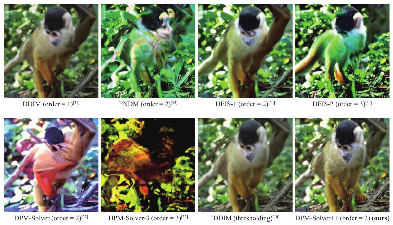
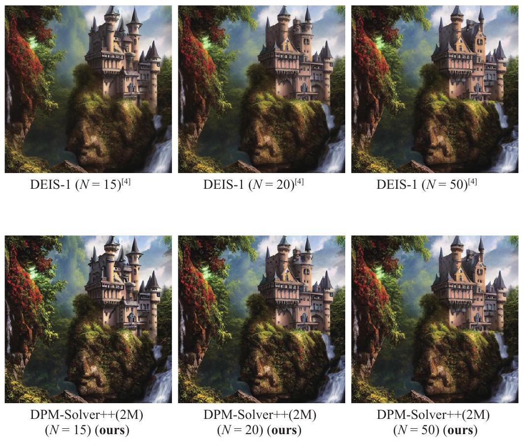
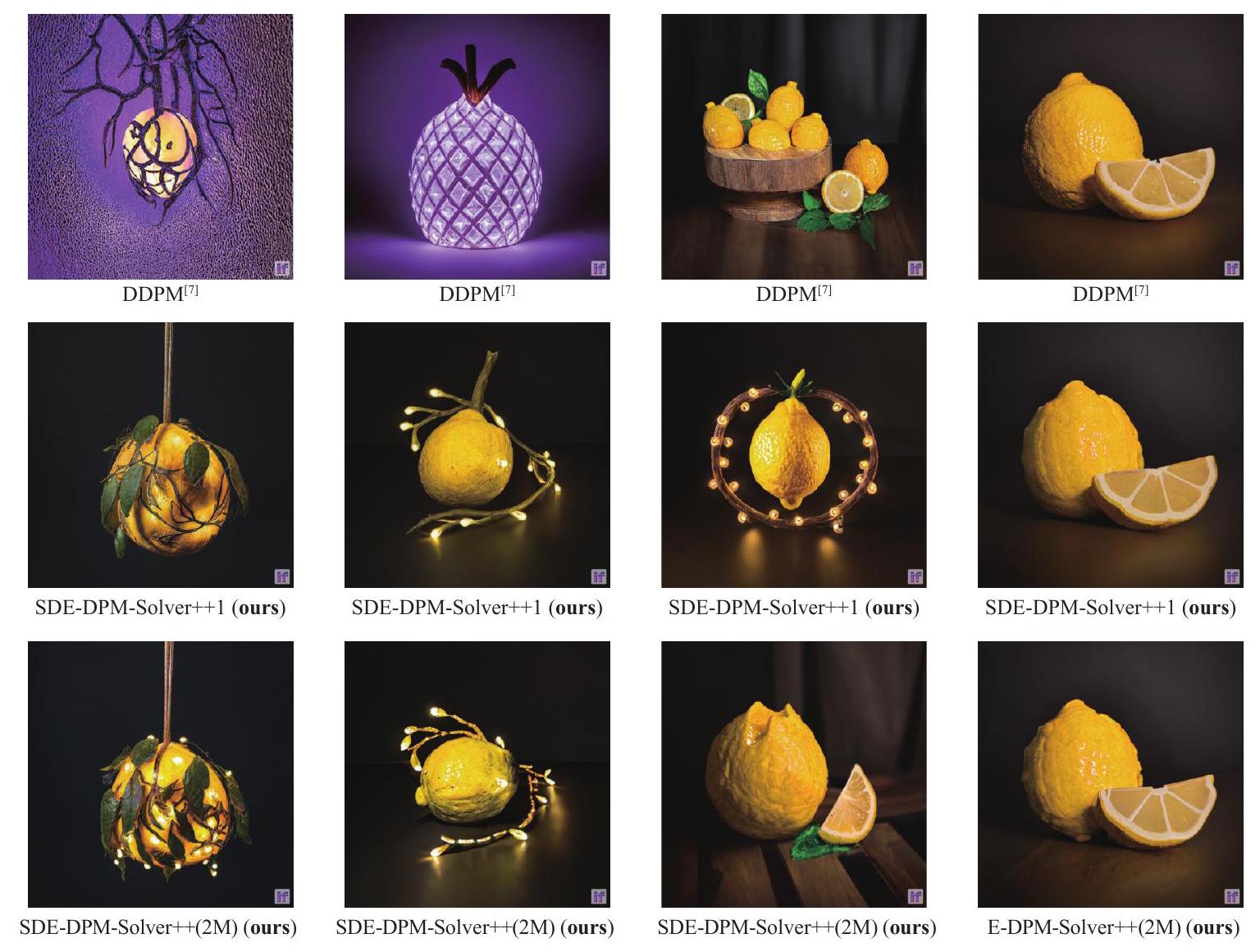
حققت نماذج الانتشار الاحتمالية (DPMs) نجاحًا ملحوظًا في توليد الصور عالية الدقة، خاصة في التطبيقات الحديثة لتوليد النص إلى صورة على نطاق واسع. تقنية أساسية لتحسين جودة العينة من DPMs هي أخذ العينات الموجهة، والتي تحتاج عادةً إلى نطاق توجيه كبير للحصول على أفضل جودة عينة. العينة السريعة المستخدمة عادةً لأخذ العينات الموجهة هي نماذج الانتشار الضبابية غير المباشرة (DDIM)، وهي حل لمعادلة تفاضلية عادية (ODE) من الدرجة الأولى تحتاج عمومًا من 100 إلى 250 خطوة للحصول على عينات عالية الجودة. على الرغم من أن الأعمال الأخيرة تقترح حلولًا عالية الترتيب مخصصة وتحقق تسريعًا إضافيًا لأخذ العينات بدون توجيه، إلا أن فعاليتها لأخذ العينات الموجهة لم يتم اختبارها جيدًا من قبل. في هذا العمل، نوضح أن العينات السريعة السابقة من الدرجة العالية تعاني من مشاكل عدم الاستقرار، بل تصبح أبطأ من DDIM عندما يزداد نطاق التوجيه. لتسريع أخذ العينات الموجهة، نقترح DPM-Solver++، وهو حل من الدرجة العالية لأخذ العينات الموجهة من DPMs. يقوم DPM-Solver++ بحل معادلة الانتشار ODE باستخدام نموذج توقع البيانات ويتبنى طرق تحديد العتبة للحفاظ على توافق الحل مع توزيع بيانات التدريب. نقترح أيضًا متغير متعدد الخطوات من DPM-Solver++ لمعالجة مشكلة عدم الاستقرار عن طريق تقليل حجم الخطوة الفعالة. تظهر التجارب أن DPM-Solver++ يمكنه توليد عينات عالية الجودة في 15 إلى 20 خطوة فقط لأخذ العينات الموجهة من DPMs في فضاء البكسل وفضاء الكامن.

الكلمات الرئيسية: نماذج الانتشار، نماذج توليد، خوارزميات أخذ العينات، حلول المعادلات التفاضلية العادية (ODE)، توليد الصور.
الاقتباس: C. Lu, Y. Zhou, F. Bao, J. Chen, C. Li, J. Zhu. DPM-Solver++: حل سريع لأخذ العينات الموجهة لنماذج الانتشار الاحتمالية. بحث الذكاء الآلي، المجلد 22، العدد 4، الصفحات 730-751، 2025.http://doi.org/10.1007/s11633-025-1562-4

1 المقدمة

حققت نماذج الانتشار الاحتمالية (DPMs) نجاحًا ملحوظًا في مهام متنوعة، مثل توليد الصور عالية الدقة ، تحرير الصور ، توليد النص إلى صورة ، توليد الصوت ، توليد ثلاثي الأبعاد ، توليد الجزيئات ، توليد الفيديو وضغط البيانات. مقارنةً بالنماذج التوليدية العميقة الأخرى مثل الشبكات التنافسية التوليدية (GANs) والمشفرات التلقائية التباينية (VAEs) ، يمكن لـ DPMs حتى تحقيق جودة عينة أفضل من خلال الاستفادة من تقنية أساسية تسمى أخذ العينات الموجهة ، والتي تستخدم نماذج توجيه إضافية لتحسين دقة العينة وتوافق العينة الشرطية. من خلال ذلك، يمكن لـ DPMs في مهام النص إلى صورة والصورة إلى صورة توليد صور فوتوغرافية واقعية وفنية عالية الدقة ترتبط ارتباطًا وثيقًا بالشرط المعطى، مما يجلب اتجاهًا جديدًا في فن الذكاء الاصطناعي.
تقوم عملية أخذ العينات من DPMs بإزالة الضوضاء تدريجيًا من متغيرات عشوائية غاوسية نقية للحصول على بيانات واضحة، والتي يمكن اعتبارها كتحويل إما لمعادلات تفاضلية عشوائية (SDEs) أو المعادلات التفاضلية العادية (ODEs) المعرفة من خلال نموذج توقع الضوضاء أو نموذج توقع البيانات. يمكن أيضًا صياغة أخذ العينات الموجهة من DPMs مع مثل هذه التحويلات من خلال دمج نموذج غير مشروط مع نموذج توجيه، حيث يتحكم معلم فرعي في نطاق نموذج التوجيه (أي، نطاق التوجيه). الطريقة المستخدمة عادة لأخذ العينات الموجهة هي نماذج الانتشار الضبابية غير المباشرة (DDIM) ، والتي ثبت أنها حل لمعادلة تفاضلية عادية من الدرجة الأولى ، وعادة ما تحتاج إلى 100 إلى 250 خطوة من تقييمات الشبكة العصبية الكبيرة للتقارب، مما يستغرق وقتًا طويلاً.
يمكن أن تولد حلول المعادلات التفاضلية العادية عالية الترتيب عينات عالية الجودة في 10 إلى 20 خطوة لأخذ العينات بدون توجيه. ومع ذلك، لم يتم فحص فعاليتها لأخذ العينات الموجهة بعناية من قبل. في هذا العمل، نوضح أن الحلول عالية الترتيب السابقة لـ DPMs تولد عينات غير مرضية لأخذ العينات الموجهة، حتى أسوأ من الحل البسيط من الدرجة الأولى DDIM. نحدد تحديين لتطبيق
hلول عالية الترتيب على أخذ العينات الموجهة: 1) نطاق التوجيه الكبير يضيق دائرة التقارب للحلول عالية الترتيب، مما يجعلها غير مستقرة؛ و 2 الحل المتقارب لا يقع في نفس النطاق مع البيانات الأصلية (المعروفة أيضًا باسم “عدم تطابق التدريب والاختبار” ).
استنادًا إلى الملاحظات، نقترح DPM-Solver++، وهو حل سريع لمعادلة تفاضلية عادية للانتشار بدون تدريب لأخذ العينات الموجهة. نجد أن معلمة DPM تؤثر بشكل حاسم على جودة الحل. بعد ذلك، نقوم بحل معادلة الانتشار ODE المعرفة بواسطة نموذج توقع البيانات، الذي يتوقع البيانات النظيفة بناءً على الضوضاء. نستخرج حلاً عالي الترتيب لحل ODE باستخدام معلمة توقع البيانات، ونتبنى طرق تحديد العتبة الديناميكية لتخفيف مشكلة عدم تطابق التدريب والاختبار. علاوة على ذلك، نطور حلاً متعدد الخطوات يستخدم أحجام خطوات أصغر لمعالجة عدم الاستقرار.
كما هو موضح في الأشكال 1 و 2، يمكن لـ DPM-Solver++ توليد عينات عالية الجودة في 15 خطوة فقط، وهو أسرع بكثير من جميع العينات السابقة بدون تدريب لأخذ العينات الموجهة. تظهر نتائجنا التجريبية الإضافية أن DPM-Solver++ يمكنه توليد عينات عالية الدقة تقريبًا والتقارب في 15 إلى 20 خطوة فقط، لمجموعة واسعة من تطبيقات أخذ العينات الموجهة، بما في ذلك كل من DPMs في فضاء البكسل وفضاء الكامن.

2 نماذج الانتشار الاحتمالية

في هذا القسم، نستعرض DPMs وطرق أخذ العينات الخاصة بها.

2.1 أخذ العينات السريع لـ DPMs بواسطة معادلات الانتشار ODEs

تقوم DPMs بإضافة ضوضاء غاوسية تدريجيًا إلى متغير عشوائي بُعدي لإزعاج توزيع البيانات المجهولة المقابل في الوقت 0 إلى توزيع طبيعي بسيط في الوقت لبعض . توزيع الانتقال في كل وقت يحقق حيث
ونسبة الإشارة إلى الضوضاء (SNR) تنخفض بشكل صارم بالنسبة لـ. يمكن كتابة المعادلة (1) كـ حيث . المعلمة: توقع الضوضاء وتوقع البيانات. تتعلم DPMs استعادة البيانات
استنادًا إلى الإدخال الضوضائي مع إجراء إزالة الضوضاء المتسلسل. هناك طريقتان بديلتان لتعريف النموذج. يحاول نموذج توقع الضوضاء توقع الضوضاء من البيانات ، والذي يقوم بتحسين المعلمة من خلال الهدف التالي : حيث
، و 0 هو دالة وزن. بدلاً من ذلك، فإن نموذج الشكل 1 الحلول عالية الترتيب السابقة غير مستقرة لأخذ العينات الموجهة: العينات تستخدم DPMs المدربة مسبقًا
على ImageNet مع نطاق توجيه المصنف 8.0، متنوعًا بين عينات مختلفة (وأوامر حل مختلفة) مع 15 تقييمًا فقط. †: DDIM مع تحديد العتبة الديناميكية . يمكن أن تولد DPM-Solver++ المقترحة (المفصلة في الخوارزمية 2) عينات أفضل من DDIM من الدرجة الأولى، بينما تكون العينات عالية الترتيب الأخرى أسوأ من DDIM. (الأشكال الملونة متاحة في النسخة الإلكترونية على https://link.springer.com/journal/11633) نموذج توقع البيانات
يتوقع البيانات الأصلية استنادًا إلى الضوضاء ، وعلاقتها بـ مقدمة بواسطة . معادلات الانتشار ODEs. يمكن تنفيذ أخذ العينات بواسطة DPMs من خلال حل الانتشار
، والذي يكون عمومًا أسرع من طرق أخذ العينات الأخرى. بشكل محدد، يتطلب أخذ العينات بواسطة معادلات الانتشار ODEs تحويل المعادلة ODE التالية
مع تغيير من إلى 0: والمعادلة المعادلة للانتشار ODE بالنسبة لنموذج توقع البيانات
هي الشكل 2 حلول مختلفة لـ DeepFloyd-IF
(أخذ العينات الموجهة في فضاء البكسل). يمكن أن تولد DPM-Solver++(2M) المقترحة عينات أفضل من العينات الأخرى. DPM-Solver++1 تعادل DDIM مع خاصة ، كما هو مفصل في القسم 6.1. (الأشكال الملونة متاحة في النسخة الإلكترونية على https://link.springer.com/journal/11633)
حيث ، والمعاملات هي .

2.2 أخذ العينات الموجهة لـ DPMs

أخذ العينات الموجهة هي تقنية مستخدمة على نطاق واسع لتطبيق نماذج الانتشار الشرطي، والتي تكون مفيدة في تطبيقات تحويل النص إلى صورة، وتحويل صورة إلى صورة، وتحويل فئة إلى صورة. نظرًا لمتغير الحالة تحدد العينة الموجهة نموذج توقع الضوضاء الشرطي هناك نوعان من طرق أخذ العينات الموجهة، اعتمادًا على ما إذا كانت تتطلب نموذج مصنف. توجيه المصنف يستفيد من مصنف مدرب مسبقًا لتعريف نموذج توقع الضوضاء الشرطية بواسطة
أين هو مقياس التوجيه. في الممارسة العملية، فإن عادة ما يُفضل لتحسين محاذاة حالة العينة 10] للتوجيه في أخذ العينات. توجيه بدون مصنف يشارك نفس النموذج المعلم ، لنماذج توقع الضوضاء غير المشروطة والمشروطة، حيث المدخلات لنموذج غير المشروط هو عنصر نائب خاص يتم تعريف النموذج الشرطي المقابل بواسطة
ثم يمكن سحب العينات عن طريق حل المعادلة التفاضلية العادية (3) مع بدلاً من . دي دي آي إم هو حل نموذجي لأخذ العينات الموجهة، والذي يولد عينات في بضع مئات من الخطوات.

2.3 المحللات الأسية وحلول المعادلات التفاضلية العادية عالية الرتبة

تم إظهاره في الأعمال الأخيرة أن حلول المعادلات التفاضلية العادية المستندة إلى المدمجات الأسية تتقارب بشكل أسرع بكثير من الحلول التقليدية لحل معادلة التفاضل غير المشروطة (3). بالنظر إلى قيمة ابتدائية في الوقت لو وآخرون استنبط الحل معادلة الانتشار ODE (3) عند الزمن كما
حيث يتم تغيير المعادلة التفاضلية العادية من الوقت النطاق إلى -نسبة الإشارة إلى الضوضاء المجال بواسطة صيغة تغيير المتغيرات. هنا، -نسبة الإشارة إلى الضوضاء هي دالة تناقصية بحتة لـ مع الدالة العكسية ، و هم
أشكال تغيير المتغير المقابلة لـ . أظهر لو وآخرون [32] أن DDIM هو حل من الدرجة الأولى لـ (7). كما اقترحوا حلاً من الدرجة العالية يسمى “DPMSolver”، والذي يمكنه توليد عينات واقعية للنموذج غير المشروط في فقط خطوات.
لسوء الحظ، فإن الكفاءة المتميزة للمحللات عالية الرتبة الحالية لا تنتقل إلى العينة الموجهة، والتي سنناقشها قريبًا.

3 تحديات للمحللات عالية الرتبة في أخذ العينات الموجهة

قبل تطوير حلول سريعة جديدة، نقوم أولاً بفحص أداء حلول المعادلات التفاضلية العادية ذات الرتبة العالية الموجودة ونبرز التحديات.
التحدي الأول هو أن مقياس التوجيه الكبير يتسبب في عدم استقرار الحلول عالية الرتبة. كما هو موضح في الشكل 1، بالنسبة لمقياس توجيه كبير و 15 تقييمًا للوظائف، حلول المعادلات التفاضلية ذات الانتشار من الرتبة العالية السابقة تنتج صورًا منخفضة الجودة. جودة عيناتهم أسوأ حتى من DDIM من الدرجة الأولى. علاوة على ذلك، تصبح جودة العينة أسوأ كلما زادت درجة الحل.
بشكل بديهي، قد تعزز مقاييس التوجيه الكبيرة كل من المخرجات والمشتقات للنموذج. في (5). تؤثر مشتقات النموذج على نطاق التقارب لمحللات المعادلات التفاضلية العادية، وقد تتسبب التضخيمات في حاجة محللات المعادلات التفاضلية العادية من الدرجة العالية إلى أحجام خطوات أصغر بكثير للتقارب، وبالتالي قد تؤدي محللات الدرجة العالية إلى أداء أسوأ من محلل الدرجة الأولى. علاوة على ذلك، تتطلب المحللات من الدرجة العالية مشتقات من الدرجة العالية، والتي تكون عمومًا أكثر حساسية للتضخيمات. وهذا يضيق دائرة التقارب أكثر.
التحدي الثاني هو مشكلة “عدم تطابق التدريب والاختبار” توجد البيانات في فترة محدودة (على سبيل المثال، لبيانات الصورة). ومع ذلك، فإن المقياس الكبير للإرشاد يدفع نموذج توقع الضوضاء الشرطية بعيدًا عن الضوضاء الحقيقية، مما يجعل العينة (أي، الحل المتقارب للمعادلات التفاضلية الخاصة بالانتشار) أن تخرج عن الحدود. في هذه الحالة، تكون الصور الناتجة مشبعة وغير طبيعية. .

4 تصميم عينات سريعة بدون تدريب لأغراض التوجيه

في هذا القسم، نصمم حلول ODE جديدة من الدرجة العالية للتشتت من أجل تسريع عملية العينة الموجهة. كما تم مناقشته في القسم 3، فإن الحلول السابقة من الدرجة العالية تعاني من عدم الاستقرار ومشاكل “عدم تطابق التدريب والاختبار” عند استخدام مقاييس توجيه كبيرة. تنشأ مشكلة “عدم تطابق التدريب والاختبار” من ODE نفسه، ونجد أن تهيئة ODE أمر حاسم لضمان أن تكون الحلول المتقاربة محدودة. بينما تم تصميم الحلول السابقة من الدرجة العالية لنموذج توقع الضوضاء. نحن نحل المعادلة التفاضلية (4) لنموذج توقع البيانات والتي تحتوي على بعض المزايا، وتتوفر أيضًا طرق تحديد العتبة للحفاظ على العينات ضمن الحدود. . نقترح أيضًا حلًا متعدد الخطوات-
للتعامل مع مشكلة عدم الاستقرار.

4.1 تصميم الحلول بواسطة نموذج توقع البيانات

نتبع الرموز في [32]. بالنظر إلى تسلسل يتناقص من إلى وقيمة أولية يهدف الحل إلى حساب تسلسل بشكل تكراري لتقريب الحل الدقيق في كل وقت “، والقيمة النهائية هو العينة المقدرة بواسطة معادلة التفاضل الجزئي. دلالة لـ .
لحل معادلة الانتشار التفاضلية بالنسبة لـ في (4)، نقترح أولاً صياغة مبسطة للحل الدقيق لمعادلات التفاضل الجزئي المتعلقة بالانتشار. أدناه. هذه الصياغة تحسب بدقة الحد الخطي في (4) ولا يتبقى سوى تكامل موزون أسي لـ . يدل على كشكل تغيير المتغير لـ لـ لدينا:
الاقتراح 1 (الحل الدقيق لمعادلات الانتشار التفاضلية) ، الدليل في الملحق أ). بالنظر إلى قيمة أولية في الوقت الحل في الوقت معادلات الانتشار ODEs في (4) هي
نظرًا لأن معادلات الانتشار ODEs في (3) و (4) متكافئة، فإن صيغ الحلول الدقيقة في (7) و (8) أيضًا متكافئة. ومع ذلك، من منظور تصميم حلول ODE، فإن هاتين الصيغتين مختلفتان. أولاً، (7) تحسب بالضبط الحد الخطي بينما (8) تحسب بدقة مصطلح خطي آخر . علاوة على ذلك، لتصميم حلول المعادلات التفاضلية العادية، يحتاج (7) إلى تقريب التكامل بينما (8) يحتاج إلى التقريب ، وهذان التكاملان مختلفان (تذكر أن لذلك، فإن الحلول ذات الرتبة العالية المستندة إلى (7) و (8) تختلف بشكل أساسي. نقترح أيضًا الطريقة العامة لتصميم حلول ODE ذات الرتبة العالية استنادًا إلى (8) أدناه.
بالنظر إلى القيمة السابقة في الوقت الهدف من حلنا هو تقريب الحل الدقيق في الوقت . يدل على كـ المشتقات الكلية من الرتبة -ث بالنسبة إلى . ل ، أخذ -توسيع تايلور من الدرجة لـ بالنسبة إلى واستبداله في (8) مع و لدينا
أين يتم تعريفه على النحو التالي:
والتكامل يمكن حسابه تحليليًا بواسطة التكامل بالتجزئة (المفصل في الملحق . لذلك، لتصميم الـ حل معادلة تفاضلية من الرتبة -th، نحتاج فقط إلى تقدير المشتقات من الرتبة -th لـ بعد حذف مصطلحات الخطأ من الدرجة العالية، والتي هي تقنيات مدروسة جيدًا وقد ناقشناها بالتفصيل في القسم 4.2. حالة خاصة هي حيث يكون الحل هو نفسه ونناقش ذلك في القسم 6.1.
لـ نستخدم تقنية مشابهة لـ DPM-Solver لتقدير المشتق . على وجه التحديد، نقدم خطوة زمنية وسيطة إضافية بين و واجمع قيم الدالة عند و لتقريب المشتق، وهو الأسلوب القياسي لمحللات المعادلات التفاضلية ذات الخطوة الواحدة بشكل عام، نحن بحاجة إلى خطوات الزمن و ) الذي يفي بـ . يتم اقتراح الخوارزمية التفصيلية في الخوارزمية 1، حيث نجمع القيمة السابقة في الوقت مع القيمة المتوسطة في الوقت لحساب القيمة في الوقت .
الخوارزمية 1. DPM-Solver++(2S).
يتطلب: القيمة الأولية خطوات الزمن و نموذج توقع البيانات .
  1. لـ إلى يفعل
  2. نهاية لـ
  3. عودة
الخوارزمية 2. DPM-Solver++(2M).
يتطلب: القيمة الأولية خطوات الزمن نموذج توقع البيانات .
  1. يدل على لـ
  2. قم بتهيئة مخزن فارغ
  3. لـ إلى يفعل
  4. ، )
  5. إذا ، ثم
  6. نهاية لـ
  7. عودة
نطلق على الخوارزمية اسم DPM-Solver++(2S)، مما يعني أن الحل المقترح هو طريقة من الدرجة الثانية ذات خطوة واحدة. نقدم الضمان النظري لترتيب التقارب في الملحق A. من أجل كما تم مناقشته في القسم 3، قد تكون الحلول عالية الرتبة غير مناسبة لمقاييس التوجيه الكبيرة، وبالتالي نعتبر بشكل أساسي في هذا العمل، وترك الحلول للرتب الأعلى للدراسة في المستقبل.
علاوة على ذلك، نقدم مقارنة نظرية بين DPM-Solver-2 و DPM-Solver++(2S) في الملحق ب. نجد أن DPM-Solver++(2S) لديه ثابت أصغر قبل حدود الخطأ عالية الرتبة، وبالتالي عمومًا لديه خطأ تفريق أصغر من DPM-Solver-2.

4.2 من خطوة واحدة إلى خطوات متعددة

في كل خطوة (من إلى يتطلب الحل المقترح بخطوة واحدة تقييمين متتاليين لوظيفة الشبكة العصبية. علاوة على ذلك، القيم المتوسطة تُستخدم مرة واحدة فقط ثم تُdiscard. هذه الطريقة تفقد المعلومات السابقة وقد تكون غير فعالة. في هذا القسم، نقترح حلاً لمعادلة تفاضلية من الدرجة الثانية يستخدم المعلومات السابقة في كل خطوة.
بشكل عام، لتقريب المشتقات في (9) لـ هناك نهج سائد آخر : طرق متعددة الخطوات (مثل طرق آدامز-باشفورث). بالنظر إلى القيم السابقة في الوقت تقوم الطرق متعددة الخطوات بإعادة استخدام القيم السابقة لتقريب المشتقات ذات الرتبة العالية. تعتبر الطرق متعددة الخطوات أكثر كفاءة من الناحية التجريبية مقارنة بالطرق ذات الخطوة الواحدة، خاصةً عندما يكون عدد تقييمات الدالة محدودًا. .
نجمع بين تقنيات تصميم الحلول متعددة الخطوات مع توسعات تايلور في (9) ونقترح أيضًا حلاً متعدد الخطوات من الدرجة الثانية لمعادلات التفاضل الجزئي الخاصة بالانتشار مع تم اقتراح الخوارزمية التفصيلية في الخوارزمية 2، حيث نقوم بدمج القيم السابقة و لحساب القيمة بدون قيم وسيطة إضافية. نحن نسمي الخوارزمية DPMSolver++(2M)، مما يعني أن الحل المقترح هو حل متعدد الخطوات من الدرجة الثانية. كما نقدم ضمانًا نظريًا مفصلًا لترتيب التقارب، والذي تم ذكره في الملحق A.
لميزانية ثابتة من إجمالي عدد تقييمات الدوال، يمكن أن تستخدم الطرق متعددة الخطوات خطوات، بينما طرق الخطوة الواحدة من الرتبة -th يمكن أن تستخدم فقط ما لا يزيد عن خطوات. لذلك، كل حجم خطوة
طرق متعددة الخطوات حوالي من تلك الطرق ذات الخطوة الواحدة، لذا فإن حدود الخطأ من الرتبة العالية في (9) من طرق الخطوات المتعددة قد تكون أيضًا أصغر من تلك الخاصة بطرق الخطوة الواحدة. نوضح في القسم 7.1 أن طرق الخطوات المتعددة أفضل قليلاً من طرق الخطوة الواحدة.

4.3 دمج العتبة مع DPMSolver++

بالنسبة لتوزيعات البيانات المحدودة (مثل بيانات الصور)، فإن طرق العتبة يمكن أن تدفع العينات الخارجة عن الحدود إلى الداخل وتقلل بطريقة ما من التأثير السلبي لمقياس التوجيه الكبير. بشكل محدد، تحدد طرق العتبة نموذج توقع بيانات مقطوعة. عن طريق قص النموذج الأصلي عنصرًا بعنصر ضمن حدود البيانات، مما يؤدي إلى تحسين جودة العينة عند استخدام مقاييس توجيه كبيرة . تم تصميم DPM-Solver++ المقترح لدينا لـ نموذج، يمكننا ببساطة دمج طرق العتبة مع DPM-Solver++.

5 حلول سريعة لمعادلات التفاضل العشوائية الانتشارية

يمكن تنفيذ أخذ العينات بواسطة نماذج الانتشار بدلاً من ذلك من خلال حل معادلات الانتشار العشوائية. :
أين هو عملية وينر العكسية الزمن من إلى 0. في هذا القسم، نعتبر معادلات الانتشار SDEs بالنسبة لـ logSNR واشتق الحلول من الدرجة الثانية المقابلة.
يدل على كعملية وينر المقابلة بالنسبة لـ للتبسيط، نُشير إلى ، ). لنماذج الانتشار من نوع VP (أي، لدينا و . كـ و معادلات سوبيرتيتية الانتشار بالنسبة لـ هو
من خلال تطبيق صيغة تغيير الثوابت، يمكننا اشتقاق الحل الدقيق لمعادلات SDEs الانتشار كما يلي:
الاقتراح 2 (الحل الدقيق لمعادلات الانتشار العشوائية، الإثبات في الملحق أ). بالنظر إلى قيمة ابتدائية في الوقت الحل في الوقت لانتشار المعادلات التفاضلية العشوائية في (11) هو
علاوة على ذلك، يمكننا حساب تكامل إيتو بواسطة
أين . وبالتالي، يمكننا تفكيك التكامل بالنسبة لـ أو للحصول على الحلول المقابلة لمعادلات SDE الانتشار، والتي تم تقديمها أدناه. للتبسيط، نوضح أن .

حل-س-دي-دي-بي-إم-1.

دع من خلال افتراض لدينا

محلّل SDE-DPM-Solver++1.

دع من خلال افتراض لدينا

SDE-DPM-Solver-2M.

دع افترض أن لدينا حلاً سابقاً مع مخرجات نموذجها في الوقت . يدل على من خلال افتراض لدينا

محلّل SDE-DPM-Solver++(2M).

دع افترض أن لدينا حلاً سابقاً مع مخرجات نموذجها في الوقت . يدل على من خلال افتراض لدينا

6 العلاقة مع طرق أخذ العينات السريعة الأخرى

في جوهرها، يمكن فهم جميع طرق أخذ العينات بدون تدريب لنماذج الانتشار على أنها إما تفكيك معادلات الانتشار العشوائية. أو تفريق معادلات تفاضلية للانتشار نظرًا لأن DPM-Solver++ مصمم لحل المعادلات التفاضلية العادية الخاصة بالانتشار، في هذا القسم، نناقش العلاقة بين DPM-Solver++ وحلول المعادلات التفاضلية الأخرى الخاصة بالانتشار. كما نناقش بإيجاز طرق أخذ العينات السريعة الأخرى لـ DPMs.

6.1 المقارنة مع الحلول المعتمدة على المدمجات الأسية

الإصدار العام من DDIM مع هو
حلول المعادلات التفاضلية العادية السريعة المتطورة السابقة استخدام المعاملات الأسية لحل المعادلات التفاضلية العادية للانتشار مع نماذج توقع الضوضاء باختصار، هذه الحلول تقرب الحل الدقيق في (7) وتضم DDIM مع كما هو الحال في الحالة من الدرجة الأولى. أدناه نوضح أن الحالة من الدرجة الأولى لـ DPM-Solver++ هي أيضًا DDIM.
لـ (9) يصبح (بعد حذف الشروط)
لذلك، فإن DPM-Solver++ المقترح لدينا هو تعميم عالي الرتبة لـ DDIM ) فيما يتعلق بنموذج توقع البيانات حسب علمنا، لم يتم اقتراح مثل هذا التعميم من قبل. نعرض الفرق التفصيلي بين المحللات عالية الرتبة السابقة المعتمدة على المدمجات الأسية وDPM-Solver++ في الجدول 1. نؤكد أنه على الرغم من أن النسخ من الرتبة الأولى من هذه المحللات متكافئة، إلا أن النسخ عالية الرتبة من هذه المحللات تختلف بشكل كبير.
بالإضافة إلى ذلك، بالنسبة لـ DDIM مع من السهل التحقق من أن مثل هذا DDIM العشوائي يعادل SDE-DPM-Solver1. لذلك، فإن الحل المقترح SDE-DPM-Solver لدينا(2M) هو نسخة عامة من الدرجة الثانية من DDIM العشوائي من الدرجة الأولى. حسب أفضل ما لدينا
الجدول 1 مقارنة بين حلول المعادلات التفاضلية العادية ذات الانتشار العالي الترتيب المستندة إلى المعاملات الأسية، بما في ذلك DEIS حل DPM و DPM-Solver++ (خاصتنا).
دييس حل DPM DPM-Solver++ (خاص بنا) SDE-DPM-Solver++ (خاصتنا)
من الدرجة الأولى دي دي آي إم ( ) دي دي آي إم ( ) دي دي آي إم ( )
نوع النموذج
توسيع تايلور لـ لـ لـ لـ
نوع الحل (مرتفع الدرجة) متعدد الخطوات خطوة واحدة خطوة واحدة + خطوات متعددة متعدد الخطوات
المعرفة، لم يتم الكشف عن مثل هذا الاكتشاف في الأعمال السابقة.

6.2 طرق أخذ العينات السريعة الأخرى

عينات تعتمد على الانتشار عادةً ما تحتاج إلى خطوات أكثر للتقارب مقارنةً بتلك المعتمدة على معادلات تفاضلية عادية للانتشار. ، لأن مهندسي البرمجيات يقدمون المزيد من العشوائية ويجعلون إزالة الضوضاء أكثر صعوبة. تشمل طرق العينة المستندة إلى التدريب الإضافي تقطير النموذج تعلم تباينات العملية العكسية ، وخطوات تعلم العينة . ومع ذلك، فإن العينات المعتمدة على التدريب السابقة يصعب توسيع نطاقها لتشمل نماذج DPM الكبيرة المدربة مسبقًا هناك طرق أخذ عينات سريعة أخرى من خلال تعديل نماذج DPM الأصلية إلى فضاء كامن. أو مع الزخم . بالإضافة إلى ذلك، دمج نماذج DPMs مع GANs يحسن جودة العينة في الشبكات التوليدية التنافسية (GANs) وسرعة العينة في نماذج الانتشار (DPMs).
مع تطور المجال بسرعة، ظهرت العديد من التقدمات منذ أن تم نشر هذه الورقة على arXiv. بالنسبة لمولدات العينات التي لا تعتمد على التدريب والتي تستند إلى المدمجات الأسية، تم تطوير أطر موحدة للتنبؤ والتصحيح لتقليل عدد العينات إلى 10 خطوات فقط. وقد تم اقتراح طريقة محددة للنموذج لتحسين كفاءة العينة تم استكشاف دمج حلول عددية تتجاوز المعالجات الأسية في نماذج الانتشار. . ومع ذلك، يبدو أن هذه الطرق التي لا تتطلب تدريبًا تواجه حاجزًا عند حوالي 5 خطوات. مؤخرًا، حققت الطرق المعتمدة على التقطير أيضًا تقدمًا كبيرًا، حيث حققت توليد بيانات عالية الجودة في خطوتين أو حتى خطوة واحدة . في الوقت نفسه، تظهر فئات جديدة من النماذج التوليدية، بما في ذلك نماذج التناسق وأساليب مطابقة العزم الاستقرائي وقد ظهرت أيضًا. لمزيد من المقارنات مع DPM-Solver++ والأساليب ذات الصلة التي نُشرت بعد ظهور عملنا على arXiv، نُشير إلى القراء المهتمين إلى التجارب المقدمة في Zhou et al. لو وسونغ .

7 تجارب

في هذا القسم، نوضح أن DPM-Solver++ يمكن أن يسرع كل من DPMs في فضاء البكسل وDPMs في فضاء الكامن من أجل العينة الموجهة. نقوم بتغيير عدد تقييمات الدالة المختلفة (NFE) وهو عدد الاستدعاءات للنموذج. أو ومقارنة DPM-Solver++ مع أحدث تقنيات العينة السريعة السابقة لـ DPMs بما في ذلك DPM-Solver دييس ،
PNDM و DDIM . نقوم أيضًا بتحويل نماذج العمليات الديناميكية في الزمن المنفصل إلى الزمن المستمر ونستخدم هذه الحلول في الزمن المستمر. نشير إلى الملحق C للحصول على تفاصيل التنفيذ وإعدادات التجارب.
نظرًا لأن الحلول السابقة لم تختبر الأداء في العينة الموجهة، فإننا نقوم أيضًا بضبط العينات الأساسية بعناية من خلال إلغاء جدول حجم الخطوة (أي، الاختيار لخطوات الوقت). وترتيب الحل. نجد أن:
  1. بالنسبة لجدول حجم الخطوة، نبحث في خطوات الزمن في الخيارات التالية: متساوي (إعداد مستخدم على نطاق واسع في توليد الصور عالية الدقة)، موحد (المستخدمة في [32])، تقسيم موحد لدوال القدرة لـ (المستخدمة في [34]، والمفصلة في الملحق ج)، ونجد أن الخيار الأفضل هو التوزيع المتساوي . وبالتالي، نستخدم موحد لخطوات الوقت في جميع تجاربنا لجميع الحلول.
  2. نجد أنه بالنسبة لمقياس توجيه كبير، فإن الخيار الأفضل لجميع الحلول السابقة هو من الدرجة الثانية (أي DPM-Solver-2 و DEIS-1). نقوم بتقييم جميع درجات الحلول السابقة ونختار أفضل نتيجة لكل NFE في مقارنتنا. على وجه التحديد، بالنسبة لـ DPM-Solver، نبلغ عن أفضل نتيجة بين DPM-Solver-2 و DPM-Solver-3، وبالنسبة لـ DEIS، نختار الأفضل بين DEIS-1 و DEIS-2 و DEIS-3.
نحن نشغل كل من DPM-Solver++(2S) و DPM-Solver++ ونجد أنه بالنسبة لمقاييس التوجيه الكبيرة، فإن DPM-Solver++(2M) متعدد الخطوات يؤدي بشكل أفضل؛ وبالنسبة لمقاييس التوجيه الصغيرة قليلاً، فإن DPM-Solver++(2S) أحادي الخطوة يؤدي بشكل أفضل. نحن نبلغ عن أفضل النتائج لـ DPM-Solver++ وجميع العينات السابقة في الأقسام 7.1 و 7.2، والقيم التفصيلية مدرجة في الملحق D.

7.1 نماذج DPM في فضاء البكسل مع التوجيه

نقارن أولاً DPM-Solver++ مع عينات أخرى لتقنية العينة الموجهة باستخدام توجيه المصنف على ImageNet مجموعة البيانات بواسطة نماذج DPM المدربة مسبقًا نقوم بقياس جودة العينة من خلال سحب 10 آلاف عينة وحساب درجة فريدشيت إنسيبشن (FID) المستخدمة على نطاق واسع. ، حيث يشير انخفاض FID عادةً إلى جودة عينة أفضل. نحن نتبنى أيضًا طريقة العتبة الديناميكية لكل من DDIM و DPMSolver++. نحن نغير مقياس التوجيه في و 2.0، تظهر النتائج في الأشكال 3(أ)-3(ج). نجد أنه بالنسبة لمقاييس التوجيه الكبيرة، فإن جميع الترتيبات العليا السابقة
تتقارب العينات (DEIS، PNDM، DPM-Solver) بشكل أبطأ من DDIM من الدرجة الأولى، مما يظهر أن العينات عالية الدرجة السابقة غير مستقرة. بدلاً من ذلك، يحقق DPM-Solver++ أفضل أداء في تسريع الأداء لكل من مقاييس التوجيه الكبيرة والصغيرة. خاصةً بالنسبة لمقاييس التوجيه الكبيرة، يمكن لـ DPM-Solver++ أن يتقارب تقريبًا في غضون 15 NFE فقط.
كإزالة، نقارن أيضًا بين DPM-Solver-2 بخطوة واحدة، وDPM-Solver++(2S) بخطوة واحدة و-
الشكل 3 مقارنات لطرق أخذ العينات المختلفة. (أ)-(ج) جودة العينة المقاسة بواسطة FID ↓ لطرق أخذ العينات المختلفة لنماذج DPMs على ImageNet مع مقياس توجيه مختلف ، مع تغيير NFE. : النتائج من خلال دمج المحلل مع طريقة العتبة الديناميكية . (د) خطأ التقارب المقاس بواسطة معيار L2 ↓ (مقسمًا على الأبعاد) بين طرق العينة المختلفة و DDIM ذو 1000 خطوة، مع تغيير NFE، لنموذج DPM في الفضاء الكامن “الانتشار المستقر” على مجموعة التحقق من MS-COCO2014، مع مقياس التوجيه الافتراضي في رمزهم الرسمي. (تتوفر الأشكال الملونة في النسخة الإلكترونية على https://link.springer.com/journal/11633)
الشكل 4 دراسة الإزالة لـ DPM-Solver++. جودة العينة مقاسة بواسطة FID ↓ لطرق العينة المختلفة لـ DPMs على ImageNet مع مقياس التوجيه 8.0، مع تغيير NFE. (الرسوم الملونة متاحة في النسخة الإلكترونية على https://link.springer.com/journal/11633)
يفضلون على أولئك بالنسبة لـ .
2) من خطوة واحدة إلى خطوات متعددة: كما هو موضح في الشكل 4(b)، يتقارب DPM-Solver++(2M) متعدد الخطوات بشكل أسرع قليلاً من DPM-Solver++(2S) ذو الخطوة الواحدة، الذي يتقارب تقريباً في 15 NFE. تشير هذه النتيجة إلى أنه بالنسبة لأخذ العينات الموجهة مع مقياس توجيه كبير، قد تكون الطرق متعددة الخطوات أسرع من الطرق ذات الخطوة الواحدة.
3) مع أو بدون تحديد العتبة: نقارن أداء DDIM و DPM-Solver++ مع/بدون طرق تحديد العتبة في الشكل 4(c). لاحظ أن طريقة تحديد العتبة تغير النموذج وهكذا تغير أيضًا الحلول المتقاربة لمعادلات التفاضل الجزئي. أولاً، نجد أنه بعد استخدام طريقة العتبة، يمكن لمعادلة التفاضل الجزئي أن تولد عينات ذات جودة أعلى، وهو ما يتماشى مع الاستنتاج في [10]. ثانيًا، تتفوق جودة العينات لـ DPM-Solver++ مع العتبة على DPM-Solver++ بدون عتبة تحت نفس عدد تقييمات الدالة. علاوة على ذلك، عند دمجه مع العتبة، يكون DPM-Solver++ أسرع من DDIM من الدرجة الأولى، مما يظهر أن DPM-Solver++ يمكنه أيضًا تسريع العينة الموجهة بواسطة DPMs باستخدام طرق العتبة.

7.2 نماذج DPM في الفضاء الكامن مع التوجيه

نقوم أيضًا بتقييم DPM-Solver++ على نماذج DPM في الفضاء الكامن الذي أصبح شائعًا مؤخرًا بين المجتمع بسبب الكود الرسمي “stable-diffusion”. نحن نستخدم مقياس التوجيه الافتراضي في الشيفرة الرسمية الخاصة بهم. تقوم نماذج DPM في الفضاء الكامن بربط بيانات الصورة مع رمز كامن من خلال تدريب زوج من المشفرات والمفككات، ثم تدريب نموذج DPM للرمز الكامن. نظرًا لأن الرمز الكامن غير محدود، فإننا لا نطبق طريقة العتبة.
على وجه التحديد، نقوم بأخذ عينة عشوائية من 10,000 زوج من التعليقات والصور من مجموعة بيانات التحقق MS-COCO2014 ونستخدم التعليقات كظروف لرسم 10,000 صورة من نموذج “الانتشار المستقر” المدرب مسبقًا، ونرسم فقط عينة صورة واحدة لكل تعليق، وفقًا لإجراءات التقييم القياسية في [6، 11]. نجد أن جميع الحلول يمكن أن تحقق FID حوالي 15.0 إلى 16.0 حتى في 10 خطوات فقط، وهو قريب جدًا من FID المحسوب من العينات المتقاربة المبلغ عنها في الصفحة الرسمية لـ “الانتشار المستقر”. نعتقد أن ذلك يعود إلى قوة فك التشفير المدرب مسبقًا، الذي يمكنه تحويل رمز كامن غير متقارب إلى عينة صورة جيدة.
بالنسبة لنماذج DPM في الفضاء الكامن، تؤثر حلول ODE المختلفة للتشتت بشكل مباشر على سرعة التقارب في الفضاء الكامن. لمقارنة مختلف العينات لنماذج DPM في الفضاء الكامن، نقوم بمقارنة مباشرة بين الحلول المختلفة وفقًا لخطأ التقارب في الفضاء الكامن بواسطة معيار L 2 بين العينات. والحل الحقيقي (وخطأ بينهما هو ). على وجه التحديد، نقوم أولاً بأخذ عينة من 10 آلاف متغير ضوضاء من التوزيع الطبيعي القياسي ونثبتها. ثم نقوم بأخذ عينة من 10 آلاف رمز كامن بواسطة عينات DPM المختلفة، بدءًا من 10 آلاف متغير ضوضاء المثبتة. كما أن كل هذه
يمكن فهم الحلول على أنها تفكيك معادلات التفاضل الجزئي للانتشار، نقارن الرموز الكامنة المأخوذة بالحل الحقيقي من نموذج DDIM مكون من 999 خطوة مع عينات بواسطة عينات مختلفة ضمن NFE مختلفة، وتظهر النتائج في الشكل 3(d). نجد أن العينات السريعة المدعومة (DDIM و PNDM) في “الانتشار المستقر” تتقارب بشكل أبطأ بكثير من DPM-Solver++ و DEIS، ونجد أن DPM-Solver++ و DEIS من الدرجة الثانية متعددة الخطوات تحققان تسريعًا قريبًا جدًا في الفضاء الكامن. علاوة على ذلك، حيث أن “الانتشار المستقر” يستخدم بشكل افتراضي PNDM مع 50 خطوة، نجد أن DPM-Solver++ يمكن أن يحقق خطأ تقارب مشابهًا مع 15 إلى 20 خطوة فقط. نقدم أيضًا مقارنة تجريبية للصور المأخوذة بين مختلف الحلول في الملحق D، ونجد أن DPM-Solver++ يمكنه بالفعل توليد عينات صور جيدة جدًا في 15 إلى 20 خطوة فقط.

8 استنتاجات

ندرس مشكلة تسريع أخذ العينات الموجهة من نماذج الانتشار (DPMs). نوضح أن الحلول عالية الرتبة السابقة المستندة إلى نماذج توقع الضوضاء غير مستقرة بشكل غير عادي وتولد عينات بجودة أسوأ من الحل الأولي DDIM لأخذ العينات الموجهة مع مقاييس توجيه كبيرة. لمعالجة هذه المشكلة وتسريع أخذ العينات الموجهة، نقترح DPM-Solver++، وهو حل سريع لمعادلات التفاضل العشوائي بدون تدريب لأخذ العينات الموجهة. يعتمد DPM-Solver++ على معادلة التفاضل العشوائي مع نماذج توقع البيانات، والتي يمكن أن تعتمد مباشرة على طرق تحديد العتبات لتثبيت إجراء أخذ العينات بشكل أكبر. نقترح كل من النسخ ذات الخطوة الواحدة والنسخ متعددة الخطوات من DPM-Solver++. تظهر نتائج التجارب أن DPM-Solver++ يمكن أن يولد عينات عالية الدقة ويكاد يتقارب في غضون 15 إلى 20 خطوة فقط، وهو قابل للتطبيق على نماذج DPM في فضاء البكسل وفضاء الكامن.

شكر وتقدير

تم دعم هذا العمل من قبل المؤسسة الوطنية للعلوم الطبيعية في الصين (الأرقام 62276149، 92370124، 62350080، 92248303، U2341228، 62061136001 و62076147)، BNRist، الصين (رقم BNR2022RC01006)، معهد تسينغhua لGuo Qiang، صندوق نموذج CCF-BaiChuanEbtech، ومركز الحوسبة عالية الأداء، جامعة تسينغhua، الصين. كما تم دعم J. Zhu من قبل جائزة XPlorer، الصين.

إعلانات تضارب المصالح

جون زو هو محرر مساعد في أبحاث الذكاء الآلي ولم يكن له دور في المراجعة التحريرية، أو القرار بنشر هذه المقالة. وقد أعلن جميع المؤلفين أنهم ليس لديهم أي تضارب في المصالح يتعلق بهذا العمل.

الوصول المفتوح

هذه المقالة مرخصة بموجب رخصة المشاع الإبداعي.
ترخيص المشاع الإبداعي 4.0 الدولي، الذي يسمح بالاستخدام والمشاركة والتكيف والتوزيع وإعادة الإنتاج بأي وسيلة أو صيغة، طالما أنك تعطي الائتمان المناسب للمؤلفين الأصليين والمصدر، وتوفر رابطًا لترخيص المشاع الإبداعي، وتوضح ما إذا تم إجراء تغييرات.
الصور أو المواد الأخرى من طرف ثالث في هذه المقالة مشمولة في ترخيص المشاع الإبداعي للمقالة، ما لم يُشار إلى خلاف ذلك في سطر الائتمان للمادة. إذا لم تكن المادة مشمولة في ترخيص المشاع الإبداعي للمقالة وكان استخدامك المقصود غير مسموح به بموجب اللوائح القانونية أو يتجاوز الاستخدام المسموح به، فسيتعين عليك الحصول على إذن مباشرة من صاحب حقوق الطبع والنشر.
للاطلاع على نسخة من هذه الرخصة، قم بزيارةhttp://creativecommons.org/licenses/by/4.0/.

الملحق أ. براهين إضافية

أ. 1 إثبات الاقتراح 1

برهان. أخذ المشتقة بالنسبة إلى في (8) ينتج
حيث أن عدم المساواة الأخيرة تتبع من التعريفات .

أ. 2 إثبات الاقتراح 2

برهان. بالنسبة لمعادلات سوبيرتسكي العشوائية المتعلقة بنموذج توقع الضوضاء لدينا
وبالنسبة لمعادلات سوبيرتسكي العشوائية المتعلقة بنموذج توقع البيانات لدينا

أ. 3 اشتقاق حلول معادلات ستيت

الدليل. في هذا القسم، نستنتج SDE-DPM-Solver-1 و SDE-DPM-Solver++1 و SDE-DPM-Solver-2M و SDE-DPM-Solver++2M.
  1. بالنسبة لـ SDE-DPM-Solver-1، لدينا
  1. بالنسبة لـ SDE-DPM-Solver++1، لدينا
  1. بالنسبة لـ SDE-DPM-Solver-2M، لدينا
يمكننا أيضًا تطبيق نفس التقريب كما في [32] عن طريق
وهكذا لدينا
  1. بالنسبة لـ SDE-DPM-Solver++2M، لدينا
يمكننا أيضًا تطبيق نفس التقريب كما في [32] عن طريق
لذا لدينا

أ. 4 تقارب الخوارزميات

نقوم بعمل الافتراضات التالية كما في [32] لـ أي،
  1. و توجد وتكون مستمرة (ومن ثم تكون محدودة).
  2. الخريطة هو -ليبسشيتز.
  3. .
نفترض أيضًا المزيد
  1. للجميع .
ثم، كلا الخوارزميات من الدرجة الثانية:
الاقتراح 3. بموجب الافتراضات المذكورة أعلاه، عندما صغيرة بما فيه الكفاية، لدينا لكل من الخوارزميات 1 و .

أ.4.1 تقارب الخوارزمية 1

إثبات التقارب للخوارزمية 1 مشابه لذلك في DPM-Solver-2 نقدمه في هذا القسم من أجل الاكتمال.
برهان. أولاً، يعطي توسع تايلور
دع ثم يرجى ملاحظة أن
منذ محدود بعيدًا عن الصفر، و نحن نعلم
أين . ثم، يمكن تقديرها على النحو التالي:
لذا، طالما صغير بما فيه الكفاية.

أ.4.2 تقارب الخوارزمية 2

باتباع نفس خط الحجة في إثبات التقارب للخوارزمية 1، يمكننا إثبات تقارب الخوارزمية 2.
برهان. لن توسيع تايلور يعطي
أين هو ثابت يعتمد على . كما يُرجى ملاحظة أن
منذ محدود بعيدًا عن الصفر، و نحن نعلم
أين . ثم، يمكن تقديره على النحو التالي:
لذا، طالما صغير بما فيه الكفاية و والذي يمكن التحقق منه من خلال توسيع تايلور.

ب. المقارنة بين DPM-Solver و DPM-Solver++

في هذا القسم، نقوم بتحويل DPM-Solver++(2S) إلى الصيغة المتعلقة بنموذج توقع الضوضاء، ونقارنها مع DPM-Solver من الدرجة الثانية. .
في كل خطوة، محلل DPM من الدرجة الثانية (DPM-Solver-2 ) لديها القواعد التالية للتحديث:
بينما يحتوي DPM-Solver++(2S) على قواعد التحديث التالية:
يرجى ملاحظة أن
ثم يمكننا إعادة كتابة DPM-Solver++(2S) بالنسبة لنموذج توقع الضوضاء (انظر الملحق ب. 1 للحصول على التفاصيل):
عند المقارنة مع (B2)، يمكننا أن نجد أن الاختلاف الوحيد بين DPM-Solver-2 و DPM-Solver++(2S) هو أن DPM-Solver++(2S) يحتوي على معامل إضافي. في الحد الثاني (الذي يتوافق مع تقريب المشتق الكلي من الدرجة الأولى ). على وجه التحديد، لدينا
بينما يقوم DPM-Solver++(2S) بضرب معامل أصغر في الـ مصطلح الخطأ، الثابت السابق في مصطلح الخطأ العالي الترتيب لـ DPM-Solver++(2S) أصغر من ذلك في DPM-Solver-2. حيث أن كلاهما يعادل تفكيك من الدرجة الثانية لمعادلة الانتشار ODE، يمكن أن يؤدي الثابت الأصغر قبل مصطلح الخطأ إلى تقليل خطأ التفكيك وبالتالي يقلل من عدم الاستقرار العددي (خاصةً عند استخدام مقاييس توجيه كبيرة). لذلك، فإن استخدام نموذج توقع البيانات هو مفتاح لتثبيت العينة، وDPM-Solver++(2S) أكثر استقرارًا من DPM-Solver-2.

ب. 1 اشتقاق مفصل

يمكننا إعادة كتابة DPM-Solver++(2S) بواسطة
و
و
لذا لدينا

ج. تفاصيل التنفيذ

ج. 1 تحويل نماذج إدارة العمليات الزمنية المنفصلة إلى نماذج إدارة العمليات الزمنية المستمرة

نماذج العمليات الديناميكية في الزمن المنفصل تدريب نموذج توقع الضوضاء في خطوات زمنية ثابتة ونموذج توقع الضوضاء مُعَلم بواسطة لـ ، حيث كل يت correspond إلى القيمة في الوقت . في الممارسة العملية، تختار هذه النماذج الديناميكية للعمليات المميزة عادةً خطوات زمنية متساوية بين ، وبالتالي ، من أجل أصغر وقت هو .
علاوة على ذلك، بالنسبة لـ نحن عادةً نختار تسلسلًا ، والذي يتم تعريفه إما بجدول زمني خطي أو جدول جيب التمام . بعد الحصول على التسلسل، جدول الضوضاء يتم تعريفه بواسطة
حيث كل يتوافق مع الزمن المستمر ، أي، لتعميم المتقطع إلى النسخة المستمرة، نستخدم الاستيفاء الخطي للدالة . على وجه التحديد، لكل نحن نحدد
لذلك، يمكننا الحصول على جدول ضوضاء في الوقت المستمر مُعرّف لجميع ، المعيار و الـ . علاوة على ذلك، يتناقص بشكل صارم لـ ، وبالتالي تغيير المتغير لـ لا يزال ساريًا.
في الممارسة العملية، عادةً ما يكون لدينا و وبذلك فإن أصغر وقت هو . لذلك، نحن نحل معادلات التفاضل الجزئي الخاصة بالانتشار من الزمن إلى الوقت للحصول على عينة نهائية. يمكن أن يقلل هذا النوع من أخذ العينات من حل DDIM في الزمن المنفصل من الدرجة الأولى عند استخدام خطوة زمنية موحدة.

ج. 2 خطوات الوقت للإزالة

تم ضبط DEIS السابق فقط على بيانات منخفضة الدقة مثل CIFAR-10، والتي قد لا تكون مناسبة للبيانات عالية الدقة مثل ImageNet. ومقاييس توجيه كبيرة لعينات موجهة. من أجل مقارنة عادلة مع عينات الأساس، نقوم أولاً بدراسة الإزالة لخطوات الوقت مع نماذج DPM المدربة مسبقًا. على ImageNet وتغيير مقياس توجيه المصنف. في تجاربنا، نقوم بضبط جدول خطوات الوقت وفقًا لاختيارات دالة القوة الخاصة بهم. على وجه التحديد، دع و خطوات الزمن يرضي
أين هو معلمة فرعية. وفقًا لزانغ وتشين نبحث في بواسطة DEIS، وتظهر النتائج في الجدول C1. نجد أنه بالنسبة لجميع مقاييس التوجيه، فإن أفضل إعداد هو أي، الموحد لخطوات الزمن. نقارن أيضًا بين التوزيع المنتظم وuniform ووجد أن الزي الرسمي جدول خطوات الزمن لا يزال الخيار الأفضل. لذلك، في جميع تجاربنا، نستخدم التوزيع المتساوي للتقييمات.

ج. 3 إعدادات التجربة

نستخدم جدول زمن ثابت موحد لجميع التجارب. بشكل خاص، كما هو الحال مع DPM-Solver مصمم للزي الموحد (خطوات الوقت الوسيطة هي نصف حجم الخطوة بالنسبة لـ نقوم أيضًا بتحويل الخطوات الزمنية الوسيطة لضمان أن جميع الخطوات الزمنية متساوية. نجد أن مثل هذا التحويل يمكن أن يحسن جودة العينة لكل من DPM-Solver أحادي الخطوة و DPMSolver++ أحادي الخطوة.
نقوم بتشغيل NFE في 10 و 15 و 20 و 25 للمحللات عالية الرتبة و 50 و 100 و 250 لـ DDIM. في جميع التجارب، نقوم بحل معادلات تفاضلية تفريقية من إلى مع التداخل لجدول الضوضاء المفصل في الملحق C.1. بالنسبة لـ DEIS، نستخدم طرق لـ ، وهو أسرع طريقة في ورقتهم الأصلية، ونسميها DEIS- ، على التوالي.
بالنسبة للصورة المأخوذة في الشكل D1، نستخدم العبارة “قلعة جميلة بجانب شلال في الغابة، بواسطة جوزيف توما، لوحة غير لامعة، تتصدر الترند على آرتستيشن HQ”.

د. تفاصيل التجربة

نقوم بإدراج جميع النتائج التجريبية المفصلة في الأشكال D1-D3، والجداول D2-D3.
الجدول C1 جودة العينة مقاسة بواسطة FID ↓ على ImageNet نموذج الزمن المنفصل )، متنوعًا الطرق بين DDIM وأنواع مختلفة من DEIS تم تثبيت NFE عند 10.
طريقة مقياس التوجيه
8.0 ٧.٠ 6.0 5.0 ٤.٠ 3.0 2.0 1.0 0.0
دي دي آي إم 13.04 12.38 11.81 11.55 11.62 11.95 13.01 ١٦.٣٥ ٢٩.٣٣
DEIS-2، 19.12 14.83 12.39 10.94 10.13 9.76 9.74 11.01 ٢٠.٣٤
DEIS-2، ٣٣.٣٧ ٢٤.٦٦ 18.03 ١٣.٥٧ 11.16 10.54 10.88 ١٣.٦٧ ٢٦.٢٦
DEIS-2، ٥٥.٦٩ 44.01 ٣٣.٠٤ ٢٤.٥٠ 18.66 ١٦.٣٥ 16.87 ٢١.٩١ ٣٨.٤١
DEIS-3، 66.81 ٤٨.٧١ ٣٣.٨٩ ٢٢.٥٦ 15.84 11.96 10.18 10.19 18.70
DEIS-3، ٣٤.٥١ ٢٥.٤٢ 18.52 13.68 11.20 10.46 10.75 ١٣.٣٦ ٢٥.٥٩
DEIS-3، ٥٦.٤٩ 44.51 ٣٣.٣٤ ٢٤.٦٨ 18.72 ١٦.٣٨ 16.79 21.76 ٣٨.٠٢
دي دي آي إم
دي دي آي إم
PNDM
PNDM
PNDM
دي دي آي إم ( تجمع
DPM-Solver-2
DPM-Solver-2
DPM-Solver-2
الشكل D1 عينات باستخدام نماذج DPM في الفضاء الكامن المدربة مسبقًا (الانتشار المستقر) ) مع مقياس توجيه خالٍ من المصنفات 7.5 (الإعداد الافتراضي)، مع تغيير عينات مختلفة وعدد مختلف من تقييمات الوظائف (تتوفر الأشكال الملونة في النسخة الإلكترونية على https://link.springer.com/journal/11633)
الشكل D2 عينات من طرق أخذ العينات المختلفة لـ DPMs على ImageNet مع مقياس التوجيه 8.0 (تتوفر الأشكال الملونة في النسخة الإلكترونية على https://link.springer.com/journal/11633)
الشكل D3 حلول مختلفة لـ DeepFloyd-IF (العينة الموجهة بواسطة فضاء البكسل). يمكن لمقترحنا SDE-DPM-Solver++(2M) أن ينتج عينات أفضل من العينات الأخرى. SDE-DPM-Solver++1 يعادل DDIM مع كما هو موضح في القسم 6.1. (تتوفر الأشكال الملونة في النسخة الإلكترونية على https://link.springer.com/journal/11633)
الجدول D2 جودة العينة مقاسة بواسطة FID ↓ على ImageNet نموذج الزمن المنفصل )، متغيرًا NFE
مقياس التوجيه العتبة طريقة أخذ العينات NFE
10 15 20 ٢٥ 50 100 ٢٥٠
دي دي آي إم 13.04 11.27 10.21 9.87 9.82 9.52 9.37
PNDM 99.80 ٣٧.٥٩ 15.50 11.54
DPM-Solver-2 ١١٤.٦٢ 44.05 ٢٠.٣٣ 9.84
DPM-Solver-3 164.74 91.59 64.11 ٢٩.٤٠
لا DEIS-1 15.20 10.86 10.26 10.01
8.0 DEIS-2 19.12 11.37 10.08 9.75
DEIS-3 66.86 ٢٤.٤٨ 12.98 10.87
DPM-Solver++(S) (خاص بنا) ١٢.٢٠ 9.85 9.19 9.32
DPM-Solver++(M) (خاص بنا) ١٤.٤٤ 9.46 9.10 9.11
نعم دي دي آي إم 10.58 9.53 9.12 8.94 8.58 ٨.٤٩ 8.48
DPM-Solver++(S) (خاص بنا) 9.26 8.93 8.40 8.63
دي بي إم-سولفر++(م) (خاص بنا) 9.56 8.64 ٨.٥٠ 8.39
الجدول D2 (مستمر) جودة العينة مقاسة بواسطة FID ↓ على ImageNet نموذج الزمن المنفصل تغيير NFE
مقياس التوجيه العتبة طريقة أخذ العينات NFE
10 15 20 ٢٥ 50 100 ٢٥٠
٤.٠ دي دي آي إم 11.62 9.67 8.96 ٨.٥٨ 8.22 8.06 7.99
PNDM ٢٢.٧١ 10.03 8.69 8.47
دي بي إم – سولفر – 2 ٣٧.٦٨ 9.42 8.22 8.08
دي بي إم – سولفر – 3 ٧٤.٩٧ 15.65 9.99 8.15
لا DEIS-1 10.55 9.47 8.88 8.65
DEIS-2 10.13 9.09 8.68 8.45
DEIS-3 15.84 9.25 8.63 8.43
DPM-Solver++(S)(خاصتنا) 9.08 8.51 ٨.٠٠ 8.07
دي بي إم – سولفر ++ (م) (خاص بنا) 8.98 8.26 8.06 8.06
نعم دي دي آي إم 10.45 ٨.٩٥ 8.51 8.25 7.91 7.82 7.87
دي بي إم – سولفر بلس بلس (S) (خاصتنا) 8.94 8.26 ٧.٩٥ 7.87
DPM-Solver++(M)(خاص بنا) 8.91 8.21 7.99 7.96
2.0 دي دي آي إم 13.01 9.60 9.02 8.45 7.72 ٧.٦٠ 7.44
PNDM 11.58 8.48 8.17 7.97
دي بي إم – سولفر – 2 14.12 8.20 ٨.٥٩ 7.48
دي بي إم – سولفر – 3 21.06 ٨.٥٧ 8.19 7.85
لا DEIS-1 10.40 9.11 8.52 8.21
DEIS-2 9.74 ٨.٨٠ 8.28 8.06
DEIS-3 10.18 8.63 8.20 7.98
دي بي إم – سولفر بلس بلس (S) (خاصتنا) 9.18 8.17 ٧.٧٧ ٧.٥٦
DPM-Solver++(M)(خاص بنا) 9.19 8.47 8.17 8.07
نعم دي دي آي إم 11.19 9.20 8.42 8.05 7.65 ٧.٥٩ 7.63
DPM-Solver++(S)(خاصتنا) 9.23 8.18 7.81 ٧.٦٠
دي بي إم – سولفر بلس بلس (م) (خاص بنا) 9.28 8.56 8.28 8.18
الجدول D3 جودة العينة مقاسة بواسطة MSE ↓ على مجموعة التحقق COCO2014 (نموذج كامن ذو زمن متقطع) ، مع تغيير NFE. مقياس التوجيه هو 7.5 ، وهو الإعداد الموصى به للتشتت المستقر.
مقياس التوجيه العتبة طريقة أخذ العينات NFE
10 15 20 ٢٥ 50 100 ٢٥٠
دي دي آي إم 0.59 0.42 0.48 0.45 0.34 0.23 0.12
PNDM 0.66 0.43 0.50 0.46 0.32
دي بي إم – سولفر – 2 0.66 0.47 0.40 0.34 0.20 واحد
دي بي إم – سولفر – 3 [32] 0.59 0.48 0.43 0.37 0.23
٧.٥ لا DEIS-1 0.47 0.39 0.34 0.29 0.16 واحد
DEIS-2 0.48 0.40 0.34 0.29 0.15
DEIS-3 0.57 0.45 0.38 0.34 0.19 واحد واحد
دي بي إم – سولفر بلس بلس (S) (خاصتنا) 0.48 0.41 0.36 0.32 0.19
دي بي إم – سولفر ++ (م) (خاص بنا) 0.49 0.40 0.34 0.29 0.16
الجدول D3 (مستمر) جودة العينة مقاسة بواسطة MSE ↓ على مجموعة التحقق COCO2014 (نموذج كامن في الزمن المنفصل) )، مع تغيير NFE. مقياس التوجيه هو 7.5، وهو الإعداد الموصى به للتشتت المستقر. .
مقياس التوجيه العتبة طريقة أخذ العينات NFE
10 15 20 ٢٥ 50 100 ٢٥٠
15.0 دي دي آي إم 0.83 0.78 0.71 0.67
PNDM 0.99 0.87 0.79 0.75
DPM-Solver-2 1.13 1.08 0.96 0.86
DEIS-1 0.84 0.72 0.64 0.58
DEIS-2 0.87 0.76 0.68 0.63
دييس-3 1.06 0.88 0.78 0.73
DPM-Solver++(S) (خاص بنا) 0.88 0.75 0.68 0.61
DPM-Solver++(M) (خاص بنا) 0.84 0.72 0.64 0.58

References

[1] J. Ho, A. Jain, P. Abbeel. Denoising diffusion probabilistic models. In Proceedings of the 34th International Conference on Neural Information Processing Systems, Vancouver, Canada, Article number 574, 2020.
[2] J. Sohl-Dickstein, E. A. Weiss, N. Maheswaranathan, S. Ganguli. Deep unsupervised learning using nonequilibrium thermodynamics. In Proceedings of the 32nd International Conference on Machine Learning, Lille, France, vol.37, pp.2256-2265, 2015.
[3] Y. Song, J. Sohl-Dickstein, D. P. Kingma, A. Kumar, S. Ermon, B. Poole. Score-based generative modeling through stochastic differential equations. In Proceedings of the 9th International Conference on Learning Representations, 2021.
[4] P. Dhariwal, A. Nichol. Diffusion models beat GANs on image synthesis. In Proceedings of the 35th International Conference on Neural Information Processing Systems, Article number 672, 2021.
[5] J. Ho, C. Saharia, W. Chan, D. J. Fleet, M. Norouzi, T. Salimans. Cascaded diffusion models for high fidelity image generation. Journal of Machine Learning Research, vol. 23, no. 1, Article number 47, 2022.
[6] R. Rombach, A. Blattmann, D. Lorenz, P. Esser, B. Ommer. High-resolution image synthesis with latent diffusion models. In Proceedings of IEEE/CVF Conference on Computer Vision and Pattern Recognition, New Orleans, USA, pp. 10674-10685, 2022. DOI: 10.1109/CVPR52688.2022. 01042.
[7] C. Meng, Y. Song, J. Song, J. Wu, J. Y. Zhu, S. Ermon. SDEdit: Guided image synthesis and editing with stochastic differential equations. In Proceedings of the 10th International Conference on Learning Representations, 2022.
[8] C. Saharia, W. Chan, H. Chang, C. Lee, J. Ho, T. Salimans, D. Fleet, M. Norouzi. Palette: Image-to-image diffusion models. In Proceedings of ACM SIGGRAPH Conference Proceedings, Vancouver, Canada, Article number 15, 2022. DOI: 10.1145/3528233.3530757.
[9] M. Zhao, F. Bao, C. Li, J. Zhu. EGSDE: Unpaired image-to-image translation via energy-guided stochastic differential equations. In Proceedings of the 36th International Conference on Neural Information Processing Systems, New Orleans, USA, Article number 261, 2022.
[10] C. Saharia, W. Chan, S. Saxena, L. Li, J. Whang, E. Denton, S. K. S. Ghasemipour, B. K. Ayan, S. S. Mahdavi, R. G. Lopes, T. Salimans, J. Ho, D. J. Fleet, M. Norouzi. Photorealistic text-to-image diffusion models with deep language understanding. In Proceedings of the 36th International Conference on Neural Information Processing Systems, New Orleans, USA, Article number 2643, 2022.
[11] A. Q. Nichol, P. Dhariwal, A. Ramesh, P. Shyam, P. Mishkin, B. McGrew, I. Sutskever, M. Chen. GLIDE: Towards photorealistic image generation and editing with text-guided diffusion models. In Proceedings of the 39th International Conference on Machine Learning, Baltimore, USA, pp. 16784-16804, 2022.
[12] A. Ramesh, P. Dhariwal, A. Nichol, C. Chu, M. Chen. Hierarchical text-conditional image generation with CLIP latents, [Online], Available: https://arxiv.org/abs/2204. 06125, 2022.
[13] S. Gu, D. Chen, J. Bao, F. Wen, B. Zhang, D. Chen, L. Yuan, B. Guo. Vector quantized diffusion model for text-to-image synthesis. In Proceedings of IEEE/CVF Conference on Computer Vision and Pattern Recognition, New Orleans, USA, pp. 10686-10696, 2022. DOI: 10.1109/CVPR52688.2022.01043.
[14] J. Liu, C. Li, Y. Ren, F. Chen, Z. Zhao. DiffSinger: Singing voice synthesis via shallow diffusion mechanism. In Proceedings of the 36th AAAI Conference on Artificial Intelligence, vol.36, pp.11020-11028, 2022. DOI: 10.1609/aaai. v36i10.21350.
[15] N. Chen, Y. Zhang, H. Zen, R. J. Weiss, M. Norouzi, W. Chan. WaveGrad: Estimating gradients for waveform generation. In Proceedings of the 9th International Conference on Learning Representations, 2021.
[16] N. Chen, Y. Zhang, H. Zen, R. J. Weiss, M. Norouzi, N. Dehak, W. Chan. WaveGrad 2: Iterative refinement for text-to-speech synthesis. In Proceedings of the 22nd International Speech Communication Association, Brno, Czech Republic, pp. 3765-3769, 2021.
[17] B. Poole, A. Jain, J. T. Barron, B. Mildenhall. DreamFusion: Text-to-3D using 2D diffusion. In Proceedings of the 11th International Conference on Learning Representations, Kigali, Rwanda, 2023.
[18] Z. Wang, C. Lu, Y. Wang, F. Bao, C. Li, H. Su, J. Zhu. ProlificDreamer: High-fidelity and diverse text-to-3D generation with variational score distillation. In Proceedings of the 37th International Conference on Neural Informa-
tion Processing Systems, New Orleans, USA, Article number 368, 2023.
R. Liu, R. Wu, B. Van Hoorick, P. Tokmakov, S. Zakharov, C. Vondrick. Zero-1-to-3: Zero-shot one image to 3D object. In Proceedings of IEEE/CVF International Conference on Computer Vision, Paris, France, pp.92649275, 2023. DOI: 10.1109/ICCV51070.2023.00853.
[20] M. Xu, L. Yu, Y. Song, C. Shi, S. Ermon, J. Tang. GeoDiff: A geometric diffusion model for molecular conformation generation. In Proceedings of the 10th International Conference on Learning Representations, 2022.
[21] E. Hoogeboom, V. G. Satorras, C. Vignac, M. Welling. Equivariant diffusion for molecule generation in 3D. In Proceedings of the 39th International Conference on Machine Learning, Baltimore, USA, pp. 8867-8887, 2022.
L. Wu, C. Gong, X. Liu, M. Ye, Q. Liu. Diffusion-based molecule generation with informative prior bridges. In Proceedings of the 36th International Conference on Neural Information Processing Systems, New Orleans, USA, Article number 2647, 2022.
[23] A. Blattmann, T. Dockhorn, S. Kulal, D. Mendelevitch, M. Kilian, D. Lorenz, Y. Levi, Z. English, V. Voleti, A. Letts, V. Jampani, R. Rombach. Stable video diffusion: Scaling latent video diffusion models to large datasets, [Online], Available: https://arxiv.org/abs/2311.15127, 2023.
Y. Qin, Z. Shi, J. Yu, X. Wang, E. Zhou, L. Li, Z. Yin, X. Liu, L. Sheng, J. Shao, L. Bai, W. Ouyang, R. Zhang. WorldSimBench: Towards video generation models as world simulators, [Online], Available: https://arxiv.org/ abs/2410.18072, 2024.
[25] F. Bao, C. Xiang, G. Yue, G. He, H. Zhu, K. Zheng, M. Zhao, S. Liu, Y. Wang, J. Zhu. Vidu: A highly consistent, dynamic and skilled text-to-video generator with diffusion models, [Online], Available: https://arxiv.org/abs/2405. 04233, 2024.
L. Theis, T. Salimans, M. D. Hoffman, F. Mentzer. Lossy compression with Gaussian diffusion, [Online], Available: https://arxiv.org/abs/2206.08889, 2022.
D. P. Kingma, T. Salimans, B. Poole, J. Ho. Variational diffusion models. In Proceedings of the 35th International Conference on Neural Information Processing Systems, Article number 1660, 2021.
[28] I. J. Goodfellow, J. Pouget-Abadie, M. Mirza, B. Xu, D. Warde-Farley, S. Ozair, A. Courville, Y. Bengio. Generative adversarial nets. In Proceedings of the 28th International Conference on Neural Information Processing Systems, Montreal, Canada, vol.2, pp.2672-2680, 2014.
D. P. Kingma, M. Welling. Auto-encoding variational Bayes. In Proceedings of the 2nd International Conference on Learning Representations, Banff, Canada, 2014.
[30] J. Ho, T. Salimans. Classifier-free diffusion guidance. In Proceedings of the 34th International Conference on Neural Information Processing Systems, 2021.
[31] J. Song, C. Meng, S. Ermon. Denoising diffusion implicit models. In Proceedings of the 9th International Conference on Learning Representations, 2021.
[32] C. Lu, Y. Zhou, F. Bao, J. Chen, C. Li, J. Zhu. DPM-solver: A fast ODE solver for diffusion probabilistic model sampling in around 10 steps. In Proceedings of the 36th International Conference on Neural Information Processing
Systems, New Orleans, USA, Article number 418, 2022.
[33] T. Salimans, J. Ho. Progressive distillation for fast sampling of diffusion models. In Proceedings of the 10th International Conference on Learning Representations, 2022.
[34] Q. Zhang, Y. Chen. Fast sampling of diffusion models with exponential integrator. In Proceedings of the 11th International Conference on Learning Representations, Kigali, Rwanda, 2023.
[35] DeepFloyd: IF. GitHub, [Online], Available, https://git-hub.com/deep-floyd/IF, 2023.
[36] L. Liu, Y. Ren, Z. Lin, Z. Zhao. Pseudo numerical methods for diffusion models on manifolds. In Proceedings of the 10th International Conference on Learning Representations, 2022.
[37] M. Hochbruck, A. Ostermann. Exponential integrators. Acta Numerica, vol.19, pp.209-286, 2010. DOI: 10.1017/ S0962492910000048.
[38] K. E. Atkinson, W. Han, D. Stewart. Numerical Solution of Ordinary Differential Equations, Hoboken, USA: John Wiley & Sons, 2009.
[39] A. Jolicoeur-Martineau, K. Li, R. Piché-Taillefer, T. Kachman, I. Mitliagkas. Gotta go fast when generating data with score-based models, [Online], Available: https:// arxiv.org/abs/2105.14080, 2021.
[40] H. Tachibana, M. Go, M. Inahara, Y. Katayama, Y. Watanabe. Itô-Taylor sampling scheme for denoising diffusion probabilistic models using ideal derivatives, [Online], Available: https://arxiv.org/abs/2112.13339v1, 2021.
[41] Z. Kong, W. Ping. On fast sampling of diffusion probabilistic models, [Online], Available: https://arxiv.org/abs/ 2106.00132, 2021.
[42] F. Bao, C. Li, J. Zhu, B. Zhang. Analytic-DPM: An analytic estimate of the optimal reverse variance in diffusion probabilistic models. In Proceedings of the 10th International Conference on Learning Representations, 2022.
[43] Q. Zhang, M. Tao, Y. Chen. gDDIM: Generalized denoising diffusion implicit models. In Proceedings of the 11th International Conference on Learning Representations, Kigali, Rwanda, 2023.
[44] E. Luhman, T. Luhman. Knowledge distillation in iterative generative models for improved sampling speed, [Online], Available: https://arxiv.org/abs/2101.02388, 2021.
[45] R. San-Roman, E. Nachmani, L. Wolf. Noise estimation for generative diffusion models, [Online], Available: https://arxiv.org/abs/2104.02600, 2021.
[46] A. Q. Nichol, P. Dhariwal. Improved denoising diffusion probabilistic models. In Proceedings of the 38th International Conference on Machine Learning, pp. 8162-8171, 2021.
[47] F. Bao, C. Li, J. Sun, J. Zhu, B. Zhang. Estimating the optimal covariance with imperfect mean in diffusion probabilistic models. In Proceedings of the 39th International Conference on Machine Learning, Baltimore, USA, pp. 1555-1584, 2022.
[48] M. W. Y. Lam, J. Wang, R. Huang, D. Su, D. Yu. Bilateral denoising diffusion models, [Online], Available: https:// arxiv.org/abs/2108.11514, 2021.
[49] D. Watson, W. Chan, J. Ho, M. Norouzi. Learning fast samplers for diffusion models by differentiating through sample quality. In Proceedings of the 10th International Conference on Learning Representations, 2022.
[50] A. Vahdat, K. Kreis, J. Kautz. Score-based generative modeling in latent space. In Proceedings of the 35th International Conference on Neural Information Processing Systems, Article number 863, 2021.
[51] T. Dockhorn, A. Vahdat, K. Kreis. Score-based generative modeling with critically-damped Langevin diffusion. In Proceedings of the 10th International Conference on Learning Representations, 2022.
[52] Z. Xiao, K. Kreis, A. Vahdat. Tackling the generative learning trilemma with denoising diffusion GANs. In Proceedings of the 10th International Conference on Learning Representations, 2022.
[53] Z. Wang, H. Zheng, P. He, W. Chen, M. Zhou. DiffusionGAN: Training GANs with diffusion. In Proceedings of the 11th International Conference on Learning Representations, Kigali, Rwanda, 2023.
[54] W. Zhao, L. Bai, Y. Rao, J. Zhou, J. Lu. UniPC: A unified predictor-corrector framework for fast sampling of diffusion models. In Proceedings of the 37th International Conference on Neural Information Processing Systems, New Orleans, USA, Article number 2170, 2023.
[55] E. Liu, X. Ning, H. Yang, Y. Wang. A unified sampling framework for solver searching of diffusion probabilistic models. In Proceedings of the 12th International Conference on Learning Representations, Vienna, Austria, 2024.
[56] W. Zhao, H. Wang, J. Zhou, J. Lu. DC-Solver: Improving predictor-corrector diffusion sampler via dynamic compensation. In Proceedings of the 18th European Conference on Computer Vision, Milan, Italy, pp. 450-466, 2024. DOI: 10.1007/978-3-031-73247-8_26.
[57] K. Zheng, C. Lu, J. Chen, J. Zhu. DPM-Solver-v3: Improved diffusion ODE solver with empirical model statistics. In Proceedings of the 37th International Conference on Neural Information Processing Systems, New Orleans, USA, Article number 2423, 2023.
[58] S. Li, L. Liu, Z. Chai, R. Li, X. Tan. ERA-Solver: Error-robust Adams solver for fast sampling of diffusion probabilistic models, [Online], Available: https://arxiv.org/abs/ 2301.12935, 2023.
[59] T. Karras, M. Aittala, T. Aila, S. Laine. Elucidating the design space of diffusion-based generative models. In Proceedings of the 36th International Conference on Neural Information Processing Systems, New Orleans, USA, Article number 1926, 2022.
[60] S. Wizadwongsa, S. Suwajanakorn. Accelerating guided diffusion sampling with splitting numerical methods. In Proceedings of the 11th International Conference on Learning Representations, Kigali, Rwanda, 2023.
[61] C. Meng, R. Gao, D. Kingma, S. Ermon, J. Ho, T. Salimans. On distillation of guided diffusion models. In Proceedings of IEEE/CVF Conference on Computer Vision and Pattern Recognition, Vancouver, Canada, pp. 1429714306, 2023. DOI: 10.1109/CVPR52729.2023.01374.
[62] Z. Zhou, D. Chen, C. Wang, C. Chen. Fast ODE-based sampling for diffusion models in around 5 steps. In Proceedings of IEEE/CVF Conference on Computer Vision and Pattern Recognition, Seattle, USA, pp.7777-7786,
2024. DOI: 10.1109/CVPR52733.2024.00743.
Z. Zhou, D. Chen, C. Wang, C. Chen, S. Lyu. Simple and fast distillation of diffusion models. In Proceedings of the 38th International Conference on Neural Information Processing Systems, Vancouver, Canada, 2024.
D. Berthelot, A. Autef, J. Lin, D. A. Yap, S. Zhai, S. Hu, D. Zheng, W. Talbot, E. Gu. TRACT: Denoising diffusion models with transitive closure time-distillation, [Online], Available: https://arxiv.org/abs/2303.04248v1, 2023.
[65] J. Heek, E. Hoogeboom, T. Salimans. Multistep consistency models, [Online], Available: https://arxiv.org/abs/ 2403.06807, 2024.
[66] J. T. J. Tee, K. Zhang, H. S. Yoon, D. N. Gowda, C. Kim, C. D. Yoo. Physics informed distillation for diffusion models. Transactions on Machine Learning Research, vol. 2024, 2024.
[67] H. Zheng, W. Nie, A. Vahdat, K. Azizzadenesheli, A. Anandkumar. Fast sampling of diffusion models via operator learning. In Proceedings of the 40th International Conference on Machine Learning, Honolulu, USA, pp. 42390-42402, 2023.
[68] Y. Song, P. Dhariwal, M. Chen, I. Sutskever. Consistency models. In Proceedings of the 40th International Conference on Machine Learning, Honolulu, USA, Article number 1335, 2023.
[69] C. Lu, Y. Song. Simplifying, stabilizing and scaling con-tinuous-time consistency models. In Proceedings of the 13th International Conference on Learning Representations, Singapore, 2025.
[70] W. Luo, Z. Huang, Z. Geng, J. Z. Kolter, G. J. Qi. Onestep diffusion distillation through score implicit matching. In Proceedings of the 38th International Conference on Neural Information Processing Systems, Vancouver, Canada, pp. 115377-115408, 2024.
[71] T. Yin, M. Gharbi, R. Zhang, E. Shechtman, F. Durand, W. T. Freeman, T. Park. One-step diffusion with distribution matching distillation. In Proceedings of IEEE/CVF Conference on Computer Vision and Pattern Recognition, Seattle, USA, pp.6613-6623, 2024. DOI: 10.1109/ CVPR52733.2024.00632.
[72] L. Zhou, S. Ermon, J. Song. Inductive moment matching, [Online], Available: https://arxiv.org/abs/2503.07565, 2025.
[73] M. Heusel, H. Ramsauer, T. Unterthiner, B. Nessler, S. Hochreiter. GANs trained by a two time-scale update rule converge to a local Nash equilibrium. In Proceedings of the 31st International Conference on Neural Information Processing Systems, Long Beach, USA, pp. 6629-6640, 2017.
Cheng Lu received the B. Sc. degree in computer science and technology and the Ph. D. degree in computer science and technology advised by Professor Jun Zhu from Tsinghua University, China in 2019 and 2023, respectively.
His research interests include the theories and algorithms for large-scale deep generative models and reinforcement learning.
E-mail: lucheng.lc15@gmail.com
ORCID iD: 0009-0003-5616-0556
Yuhao Zhou received the B. Sc. degree in computer science and technology from the Department of Computer Science and Technology, Tsinghua University, China in 2020. He is currently a Ph.D. degree candidate in Tsinghua University, China.
His research interests include optimization and statistical machine learning.
E-mail: yuhaoz.cs@gmail.com
ORCID iD: 0009-0005-9553-0796
Fan Bao received the B.Sc. degree in computer science and technology from the Department of Computer Science and Technology, Tsinghua University, China in 2019, and the Ph. D. degree in computer science and technology from TSAIL Group in the Department of Computer Science and Technology, Tsinghua University, China in 2024, advised by Prof. Jun Zhu and Prof. Bo Zhang. He is currently the co-founder and CTO of Shengshu Technology, China.
His research interest is large-scale deep generative models.
E-mail: fan.bao@shengshu.ai
Jianfei Chen received the B.Sc. and Ph. D. degrees in computer science and technology from Tsinghua University, China in 2014 and 2019, respectively. He is an associate professor at Tsinghua University, China. He is also interested in probabilistic inference and modeling. He served as an Associate Editor for IEEE Transactions on Pattern Analysis and Machine Intelligence and an Area Chair in ICLR.
His research interest is efficient machine learning, including low-precision training, sparse learning, and mixture-of-experts.
ORCID iD: 0000-0002-9279-6098
Chongxuan Li received the B.Sc. and Ph. D. degrees in computer science and technology from Tsinghua University, China in 2014 and 2019, respectively. He is an associate professor at Renmin University of China, China. His works were recognized with the Outstanding Paper Award at ICLR 2022. Moreover, he served as an Associate Editor for IEEE Transactions on Pattern Analysis and Machine Intelligence and Area Chair for NeurIPS, ICLR, and ACM MM.
His research interests include generative models, deep learning, and foundation models.
E-mail: chongxuanli@ruc.edu.cn
ORCID iD: 0000-0002-0912-9076
Jun Zhu received the B. Sc. and Ph. D. degrees in computer science and technology from the Department of Computer Science and Technology, Tsinghua University, China in 2005 and 2009, where he is currently a Bosch AI professor. He was an adjunct faculty and postdoctoral fellow in the Machine Learning Department, Carnegie Mellon University, USA. He regularly serves as senior Area Chairs and Area Chairs at prestigious conferences, including ICML, NeurIPS, ICLR, IJCAI and AAAI. He was selected as “AI’s 10 to Watch” by IEEE Intelligent Systems. He is a Fellow of the IEEE and an Associate Edit-or-in-Chief of IEEE Transactions on Pattern Analysis and Machine Intelligence.
His research interest is primarily on developing machine learning methods to understand scientific and engineering data arising from various fields.
E-mail: dcszj@tsinghua.edu.cn (Corresponding author)
ORCID iD: 0000-0002-6254-2388

  1. Research Article
    Manuscript received on March 15, 2025; accepted on May 8, 2025; published online on June 23, 2025
    Recommended by Associate Editor Cheng-Lin Liu
    Colored figures are available in the online version at https://link. springer.com/journal/11633
    © The Author(s) 2025

Journal: Machine Intelligence Research, Volume: 22, Issue: 4
DOI: https://doi.org/10.1007/s11633-025-1562-4
Publication Date: 2025-06-22

DPM-Solver++: Fast Solver for Guided Sampling of Diffusion Probabilistic Models

Cheng Lu Yuhao Zhou Fan Bao Jianfei Chen Chongxuan Li Jun Zhu Department of Computer Science and Technology; BNList Center; Tsinghua-Bosch Joint Center for Machine Learning,Tsinghua University, Beijing 100084, China Shengshu Technology, Beijing 100084, China Gaoling School of AI, Renmin University of China, Beijing 100872, China

Abstract

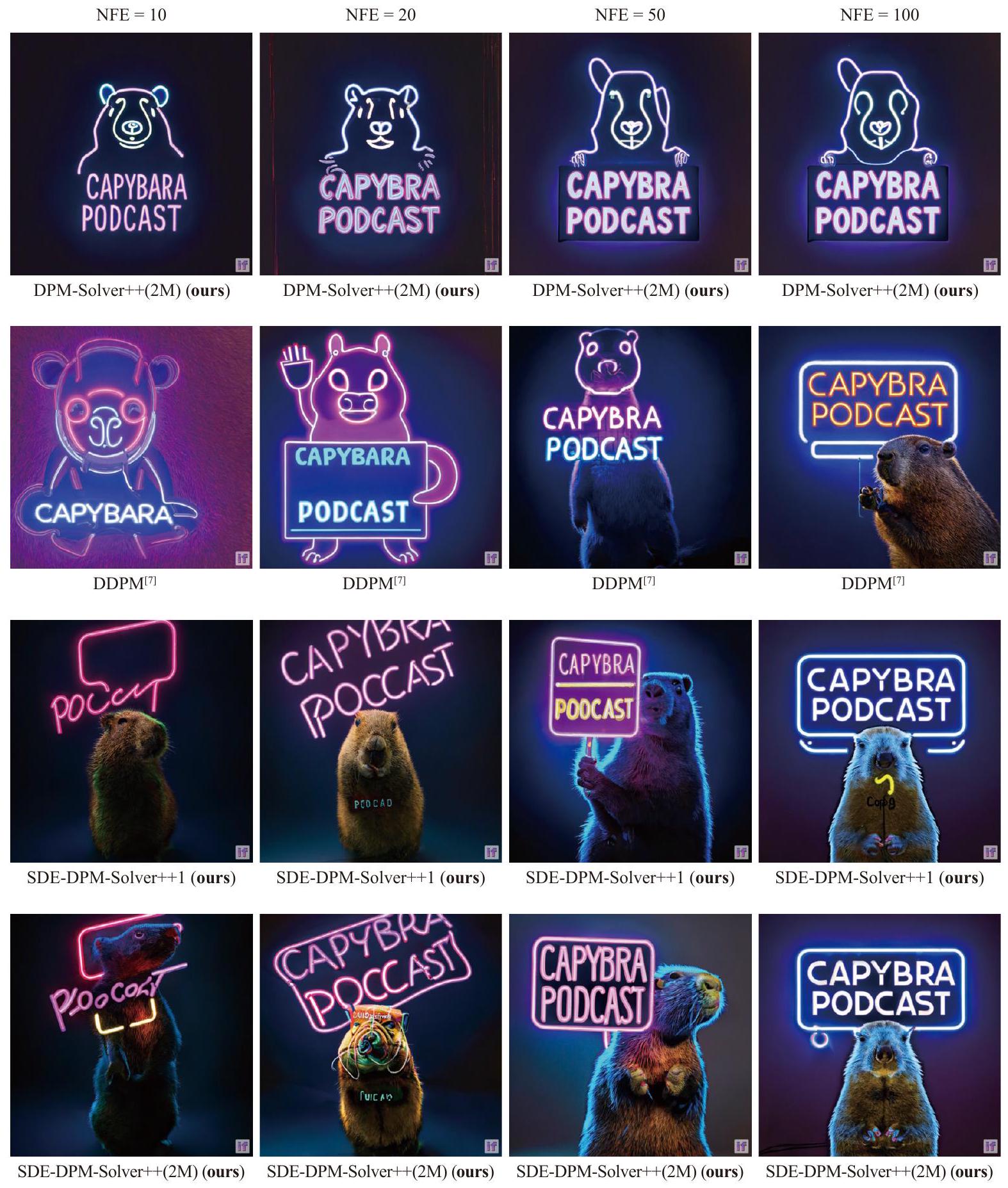
Diffusion probabilistic models (DPMs) have achieved impressive success in high-resolution image synthesis, especially in recent large-scale text-to-image generation applications. An essential technique for improving the sample quality of DPMs is guided sampling, which usually needs a large guidance scale to obtain the best sample quality. The commonly-used fast sampler for guided sampling is denoising diffusion implicit models (DDIM), a first-order diffusion ordinary differential equation (ODE) solver that generally needs 100 to 250 steps for high-quality samples. Although recent works propose dedicated high-order solvers and achieve a further speedup for sampling without guidance, their effectiveness for guided sampling has not been well-tested before. In this work, we demonstrate that previous high-order fast samplers suffer from instability issues, and they even become slower than DDIM when the guidance scale grows larger. To further speed up guided sampling, we propose DPM-Solver++, a high-order solver for the guided sampling of DPMs. DPM-Solver++ solves the diffusion ODE with the data prediction model and adopts thresholding methods to keep the solution matches training data distribution. We further propose a multistep variant of DPM-Solver++ to address the instability issue by reducing the effective step size. Experiments show that DPM-Solver++ can generate high-quality samples within only 15 to 20 steps for guided sampling by pixel-space and latent-space DPMs.

Keywords: Diffusion models, generative models, sampling algorithms, ordinary differential equation (ODE) solvers, image generation.
Citation: C. Lu, Y. Zhou, F. Bao, J. Chen, C. Li, J. Zhu. DPM-Solver++: Fast solver for guided sampling of diffusion probabilistic models. Machine Intelligence Research, vol.22, no.4, pp.730-751, 2025. http://doi.org/10.1007/s11633-025-1562-4

1 Introduction

Diffusion probabilistic models (DPMs) have achieved impressive success on various tasks, such as high-resolution image synthesis , image editing , text-to-image generation , voice synthesis , 3D generation , molecule generation , video generation and data compression . Compared with other deep generative models such as generative adversarial networks (GANs) and variational autoencoders (VAEs) , DPMs can even achieve better sample quality by leveraging an essential technique called guided sampling , which uses additional guidance models to improve the sample fidelity and the condition-sample alignment. Through it, DPMs in text-to-image and im-age-to-image tasks can generate high-resolution photorealistic and artistic images which are highly correlated to the given condition, bringing a new trend in artificial intelligence art painting.
The sampling procedure of DPMs gradually removes the noise from pure Gaussian random variables to obtain clear data, which can be viewed as discretizing either the diffusion stochastic differential equations (SDEs) or the diffusion ordinary differential equations (ODEs) defined by a parameterized noise prediction model or data prediction model . Guided sampling of DPMs can also be formalized with such discretizations by combining an unconditional model with a guidance model, where a hyperparameter controls the scale of the guidance model (i.e., guidance scale). The commonly-used method for guided sampling is denoising diffusion implicit models (DDIM) , which is proven as a first-order diffusion ODE solver , and it generally needs 100 to 250 steps of large neural network evaluations to converge, which is time-consuming.
Dedicated high-order diffusion ODE solvers can generate high-quality samples in 10 to 20 steps for sampling without guidance. However, their effectiveness for guided sampling has not been carefully examined before. In this work, we demonstrate that previous high-order solvers for DPMs generate unsatisfactory samples for guided sampling, even worse than the simple first-order solver DDIM. We identify two challenges of applying
high-order solvers to guided sampling: 1) The large guidance scale narrows the convergence radius of high-order solvers, making them unstable; and 2 the converged solution does not fall into the same range with the original data (a.k.a. “train-test mismatch” ).
Based on the observations, we propose DPM-Solver++, a training-free fast diffusion ODE solver for guided sampling. We find that the parameterization of the DPM critically impacts the solution quality. Subsequently, we solve the diffusion ODE defined by the data prediction model, which predicts the clean data given the noisy ones. We derive a high-order solver for solving the ODE with the data prediction parameterization, and adopt dynamic thresholding methods to mitigate the train-test mismatch problem. Furthermore, we develop a multistep solver which uses smaller step sizes to address instability.
As shown in Figs. 1 and 2, DPM-Solver++ can generate high-quality samples in only 15 steps, which is much faster than all the previous training-free samplers for guided sampling. Our additional experimental results show that DPM-Solver++ can generate high-fidelity samples and almost converge within only 15 to 20 steps, for a wide variety of guided sampling applications, including both pixel-space DPMs and latent-space DPMs.

2 Diffusion probabilistic models

In this section, we review DPMs and their sampling methods.

2.1 Fast sampling for DPMs by diffusion ODEs

DPMs gradually add Gaussian noise to a -dimensional random variable to perturb the corresponding unknown data distribution at time 0 to a simple normal distribution at time for some . The transition distribution at each time satisfies
where and the signal-to-noise-ratio (SNR) is strictly decreasing w.r.t. . Equation (1) can be written as , where .
Parameterization: noise prediction and data prediction. DPMs learn to recover the data based on the noisy input with a sequential denoising procedure. There are two alternative ways to define the model. The noise prediction model attempts to predict the noise from the data , which optimizes the parameter by the following objective :
where , and 0 is a weighting function. Alternatively, the data
Fig. 1 Previous high-order solvers are unstable for guided sampling: Samples use the pre-trained DPMs on ImageNet with a classifier guidance scale 8.0 , varying different samplers (and different solver orders) with only 15 function evaluations. † : DDIM with the dynamic thresholding . Our proposed DPM-Solver++ (detailed in Algorithm 2) can generate better samples than the first-order DDIM, while other high-order samplers are worse than DDIM. (Colored figures are available in the online version at https://link.springer. com/journal/11633)
prediction model predicts the original data based on the noisy , and its relationship with is given by .
Diffusion ODEs. Sampling by DPMs can be implemented by solving the diffusion , which is generally faster than other sampling methods. Specifically, sampling by diffusion ODEs needs to discretize the
following ODE with changing from to 0 :
and the equivalent diffusion ODE w.r.t. the data prediction model is
Fig. 2 Different solvers for DeepFloyd-IF (pixel-space guided sampling). Our proposed SDE-DPM-Solver++(2M) can generate better samples than other samplers. The SDE-DPM-Solver++1 is equivalent to DDIM with a special , as detailed in Section 6.1. (Colored figures are available in the online version at https://link.springer.com/journal/11633)
where , and the coefficients are .

2.2 Guided sampling for DPMs

Guided sampling is a widely-used technique to apply DPMs for conditional sampling, which is useful in text-to-image, image-to-image, and class-to-image applications . Given a condition variable , guided sampling defines a conditional noise prediction model . There are two types of guided sampling methods, depending on whether they require a classifier model. Classifier guidance leverages a pretrained classifier to define the conditional noise prediction model by
where is the guidance scale. In practice, a large is usually preferred for improving the condition-sample alignment 10] for guided sampling. Classifier-free guidance shares the same parameterized model , for the unconditional and conditional noise prediction models, where the input for the unconditional model is a special placeholder . The corresponding conditional model is defined by
Then, samples can be drawn by solving the ODE (3) with in place of . DDIM is a typical solver for guided sampling, which generates samples in a few hundreds of steps.

2.3 Exponential integrators and high-order ODE solvers

It is shown in recent works that ODE solvers based on exponential integrators converge much faster than the traditional solvers for solving the unconditional diffusion ODE (3). Given an initial value at time , Lu et al. derive the solution of the diffusion ODE (3) at time as
where the ODE is changed from the time domain to the -SNR domain by the change-of-variables formula. Here, the -SNR is a strictly decreasing function of with the inverse function , and are the
corresponding change-of-variable forms for . Lu et al.[32] showed that DDIM is a first-order solver for (7). They further proposed a high-order solver named “DPMSolver”, which can generate realistic samples for the unconditional model in only steps.
Unfortunately, the outstanding efficiency of existing high-order solvers does not transfer to guided sampling, which we shall discuss soon.

3 Challenges of high-order solvers for guided sampling

Before developing new fast solvers, we first examine the performance of existing high-order diffusion ODE solvers and highlight the challenges.
The first challenge is the large guidance scale causes high-order solvers to be instable. As shown in Fig. 1, for a large guidance scale and 15 function evaluations, previous high-order diffusion ODE solvers produce low-quality images. Their sample quality is even worse than the first-order DDIM. Moreover, the sample quality becomes even worse as the order of the solver gets higher.
Intuitively, large guidance scales may amplify both the output and the derivatives of the model in (5). The derivatives of the model affect the convergence range of ODE solvers, and the amplification may cause high-order ODE solvers to need much smaller step sizes to converge, and thus the higher-order solvers may perform worse than the first-order solver. Moreover, high-order solvers require high-order derivatives, which are generally more sensitive to the amplifications. This further narrows the convergence radius.
The second challenge is the “train-test mismatch” problem . The data lie in a bounded interval (e.g., for image data). However, the large guidance scale pushes the conditional noise prediction model away from the true noise, which in turns makes the sample (i.e., the converged solution of diffusion ODEs) to fall out of the bound. In this case, the generated images are saturated and unnatural .

4 Designing training-free fast samplers for guided sampling

In this section, we design novel high-order diffusion ODE solvers for faster guided sampling. As discussed in Section 3, previous high-order solvers have instability and “train-test mismatch” issues for large guidance scales. The “train-test mismatch” issue arises from the ODE itself, and we find the parameterization of the ODE is critical for the converged solution to be bounded. While previous high-order solvers are designed for the noise prediction model , we solve the ODE (4) for the data prediction model , which itself has some advantages and thresholding methods are further available to keep the samples bounded . We also propose a multistep solv-
er to address the instability issue.

4.1 Designing solvers by data prediction model

We follow the notations in [32]. Given a sequence decreasing from to and an initial value , the solver aims to iteratively compute a sequence to approximate the exact solution at each time , and the final value is the approximated sample by the diffusion ODE. Denote for .
For solving the diffusion ODE w.r.t. in (4), we firstly propose a simplified formulation of the exact solution of diffusion ODEs w.r.t. below. Such formulation exactly computes the linear term in (4) and only remains an exponentially-weighted integral of . Denote as the change-of-variable form of for , we have:
Proposition 1 (Exact solution of diffusion ODEs of , proof in Appendix A). Given an initial value at time , the solution at time of diffusion ODEs in (4) is
As the diffusion ODEs in (3) and (4) are equivalent, the exact solution formulations in (7) and (8) are also equivalent. However, from the perspective of designing ODE solvers, these two formulations are different. Firstly, (7) exactly computes the linear term , while (8) exactly computes another linear term . Moreover, to design ODE solvers, (7) needs to approximate the integral , while (8) needs to approximate , and these two integrals are different (recall that . Therefore, the high-order solvers based on (7) and (8) are essentially different. We further propose the general manner for designing high-order ODE solvers based on (8) below.
Given the previous value at time , the aim of our solver is to approximate the exact solution at time . Denote as the -th order total derivatives of w.r.t. . For , taking the -th Taylor expansion at for w.r.t. and substituting it into (8) with and , we have
where is defined as follows:
and the integral can be analytically computed by integral-by-parts (detailed in Appen . Therefore, to design the -th order ODE solver, we only need to estimate the -th order derivatives for after omitting the high-order error terms, which are well-studied techniques and we discussed in details in Section 4.2. A special case is , where the solver is the same as , and we discuss it in Section 6.1.
For , we use a similar technique as DPM-Solver to estimate the derivative . Specifically, we introduce an additional intermediate time step between and and combine the function values at and to approximate the derivative, which is the standard manner for singlestep ODE solvers . Overall, we need time steps and ) which satisfies . The detailed algorithm is proposed in Algorithm 1, where we combine the previous value at time with the intermediate value at time to compute the value at time .
Algorithm 1. DPM-Solver++(2S).
Require: Initial value , time steps and , data prediction model .
  1. for to do
  2. end for
  3. return
Algorithm 2. DPM-Solver++(2M).
Require: Initial value , time steps , data prediction model .
  1. Denote for
  2. . Initialize an empty buffer
  3. for to do
  4. , )
  5. If , then
  6. end for
  7. return
We name the algorithm as DPM-Solver++(2S), which means that the proposed solver is a second-order singlestep method. We present the theoretical guarantee of the convergence order in Appendix A. For , as discussed in Section 3, high-order solvers may be unsuitable for large guidance scales, thus we mainly consider in this work, and leave the solvers for higher orders for future study.
Moreover, we provide a theoretical comparison between DPM-Solver-2 and DPM-Solver++(2S) in Appendix B . We find that DPM-Solver++(2S) has a smaller constant before the high-order error terms, thus generally has a smaller discretization error than DPM-Solver-2.

4.2 From singlestep to multistep

At each step (from to ), the proposed singlestep solver needs two sequential function evaluations of the neural network . Moreover, the intermediate values are only used once and then discarded. Such method loses the previous information and may be inefficient. In this section, we propose another second-order diffusion ODE solver which uses the previous information at each step.
In general, to approximate the derivatives in (9) for , there is another mainstream approach : multistep methods (such as Adams-Bashforth methods). Given the previous values at time , multistep methods just reuse the previous values to approximate the high-order derivatives. Multistep methods are empirically more efficient than singlestep methods, especially for limited number of function evaluations .
We combine the techniques for designing multistep solvers with the Taylor expansions in (9) and further propose a multistep second-order solver for diffusion ODEs with . The detailed algorithm is proposed in Algorithm 2, where we combine the previous values and to compute the value without additional intermediate values. We name the algorithm as DPMSolver++(2M), which means that the proposed solver is a second-order multistep solver. We also present a detailed theoretical guarantee of the convergence order, which is stated in Appendix A.
For a fixed budget of the total number of function evaluations, multistep methods can use steps, while the -th order singlestep methods can only use no more than steps. Therefore, each step size
of multistep methods is around of that of singlestep methods, so the high-order error terms in (9) of multistep methods may also be smaller than those of singlestep methods. We show in Section 7.1 that the multistep methods are slightly better than singlestep methods.

4.3 Combining thresholding with DPMSolver++

For distributions of bounded data (such as the image data), thresholding methods can push out-of-bound samples inwards and somehow reduce the adverse impact of the large guidance scale. Specifically, thresholding methods define a clipped data prediction model by elementwisely clipping the original model within the data bound, which results in better sample quality for large guidance scales . As our proposed DPM-Solver++ is designed for the model, we can straightforwardly combine thresholding methods with DPM-Solver++.

5 Fast solvers for diffusion SDEs

Sampling by diffusion models can be alternatively implemented by solving diffusion SDEs :
where is the reverse-time Wiener process from to 0 . In this section, we consider the diffusion SDEs w.r.t. logSNR , and derive the corresponding second-order solvers.
Denote as the corresponding Wiener process w.r.t. . For simplicity, we denote , ). For VP-type diffusion models (i.e., ), we have and . As and , the diffusion SDEs w.r.t. is
By applying variation-of-constants formula, we can derive the exact solution of diffusion SDEs as follows:
Proposition 2 (Exact solution of diffusion SDEs, proof in Appendix A). Given an initial value at time , the solution at time of diffusion SDEs in (11) is
Moreover, we can compute the Itô-integral by
where . Thus, we can discretize the integral w.r.t. or to get the corresponding solvers for diffusion SDEs, which is presented below. For simplicity, we denote that .

SDE-DPM-Solver-1.

Let . By assuming , we have

SDE-DPM-Solver++1.

Let . By assuming , we have

SDE-DPM-Solver-2M.

Let . Assume we have a previous solution with its model output at time . Denote . By assuming , we have

SDE-DPM-Solver++(2M).

Let . Assume we have a previous solution with its model output at time . Denote . By assuming , we have

6 Relationship with other fast sampling methods

In essence, all training-free sampling methods for DPMs can be understood as either discretizing diffusion SDEs or discretizing diffusion ODEs . As DPM-Solver++ is designed for solving diffusion ODEs, in this section, we discuss the relationship between DPMSolver++ and other diffusion ODE solvers. We further briefly discuss other fast sampling methods for DPMs.

6.1 Comparison with solvers based on exponential integrators

The general version of DDIM with is
Previous state-of-the-art fast diffusion ODE solvers leverage exponential integrators to solve diffusion ODEs with noise prediction models . In short, these solvers approximate the exact solution in (7) and include DDIM with as the first-order case. Below we show that the first-order case for DPM-Solver++ is also DDIM.
For , (9) becomes (after omitting the terms)
Therefore, our proposed DPM-Solver++ is the high-order generalization of DDIM ( ) w.r.t. the data prediction model . To the best of our knowledge, such generalization has not been proposed before. We list the detailed difference between previous high-order solvers based on exponential integrators and DPM-Solver++ in Table 1. We emphasize that although the first-order versions of these solvers are equivalent, the high-order versions of these solvers are rather different.
In addition, for DDIM with , it is easy to verify that such a stochastic DDIM is equivalent to SDE-DPM-Solver1. Therefore, our proposed SDE-DPM-Solver(2M) is a second-order generalized version of the first-order stochastic DDIM. To the best of our
Table 1 Comparison between high-order diffusion ODE solvers based on exponential integrators, including DEIS , DPM-Solver and DPM-Solver++ (ours).
DEIS DPM-Solver DPM-Solver++ (ours) SDE-DPM-Solver++ (ours)
First-order DDIM ( ) DDIM ( ) DDIM ( )
Model type
Taylor expansion for for for for
Solver type (high-order) Multistep Singlestep Singlestep + multistep Multistep
knowledge, such a finding is not revealed in previous works.

6.2 Other fast sampling methods

Samplers based on diffusion generally need more steps to converge than those based on diffusion ODEs , because SDEs introduce more randomness and make denoising more difficult. Samplers based on extra training include model distillation , learning reverse process variances , and learning sampling steps . However, previous training-based samplers are hard to scale-up to pre-trained large DPMs . There are other fast sampling methods by modifying the original DPMs to a latent space or with momentum . In addition, combining DPMs with GANs improves the sample quality of GANs and sampling speed of DPMs.
As the field is evolving rapidly, several advancements have emerged since this paper was made available on arXiv. For training-free samplers based on exponential integrators, unified predictor-corrector frameworks have been developed to reduce sampling to within 10 steps , and a model-specific method has been proposed to improve the sampling efficiency . Numerical solvers beyond exponential integrators have also been explored and integrated into diffusion models . Nevertheless, these training-free methods seem to encounter a barrier at around 5 steps. Recently, distillation-based methods have also made significant progress, achieving high-quality data generation in two steps or even a single step . Meanwhile, new classes of generative models, including consistency models and inductive moment matching approaches , have also emerged. For further comparisons with DPM-Solver++ and related methods published after our work appeared on arXiv, we refer interested readers to the experiments presented in Zhou et al. , Lu and Song .

7 Experiments

In this section, we show that DPM-Solver++ can speed up both the pixel-space DPMs and the latent-space DPMs for guided sampling. We vary different number of function evaluations (NFE) which is the number of calls to the model or , and compare DPM-Solver++ with the previous state-of-the-art fast samplers for DPMs including DPM-Solver , DEIS ,
PNDM and DDIM . We also convert the discretetime DPMs to the continuous-time and use these continu-ous-time solvers. We refer to Appendix C for the detailed implementations and experiment settings.
As previous solvers did not test the performance in guided sampling, we also carefully tune the baseline samplers by ablating the step size schedule (i.e., the choice for the time steps and the solver order. We find that:
  1. For the step size schedule, we search the time steps in the following choices: uniform (a widely-used setting in high-resolution image synthesis), uniform (used in [32]), uniform split of the power functions of (used in [34], detailed in Appendix C), and we find that the best choice is uniform . Thus, we use uniform for the time steps in all of our experiments for all of the solvers.
  2. We find that for a large guidance scale, the best choice for all the previous solvers is the second-order (i.e., DPM-Solver-2 and DEIS-1). We evaluate all orders of the previous solvers and select the best result for each NFE in our comparison. Specifically, for DPM-Solver, we report the best result among DPM-Solver-2 and DPM-Solv-er-3, and for DEIS, we select the best among DEIS-1, DEIS-2, and DEIS-3.
We run both DPM-Solver++(2S) and DPM-Solver++ , and we find that for large guidance scales, the multistep DPM-Solver++(2M) performs better; and for a slightly small guidance scales, the singlestep DPM-Solver++(2S) performs better. We report the best results of DPM-Solver++ and all of the previous samplers in Sections 7.1 and 7.2, the detailed values are listed in Appendix D .

7.1 Pixel-space DPMs with guidance

We firstly compare DPM-Solver++ with other samplers for the guided sampling with classifier-guidance on ImageNet dataset by the pretrained DPMs . We measure the sample quality by drawing 10 K samples and computing the widely-used Fréchet inception distance (FID) score , where lower FID usually implies better sample quality. We also adopt the dynamic thresholding method for both DDIM and DPMSolver++. We vary the guidance scale in and 2.0, the results are shown in Figs.3(a)-3(c). We find that for large guidance scales, all the previous high-order
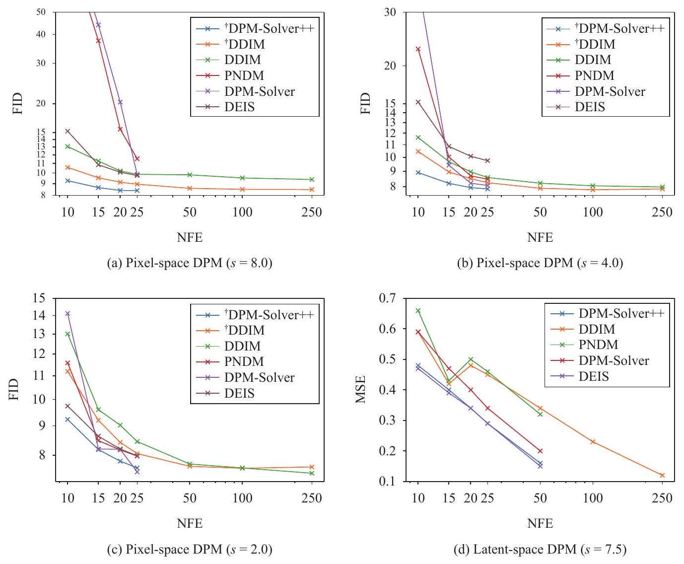
samplers (DEIS, PNDM, DPM-Solver) converge slower than the first-order DDIM, which shows that previous high-order samplers are unstable. Instead, DPM-Solver++ achieves the best speedup performance for both large guidance scales and small guidance scales. Especially for large guidance scales, DPM-Solver++ can almost converge within only 15 NFE .
As an ablation, we also compare the singlestep DPM-Solver-2, the singlestep DPM-Solver++(2S) and the mul-
Fig. 3 Comparsions of different sampling methods. (a)-(c) Sample quality measured by FID ↓ of different sampling methods for DPMs on ImageNet with different guidance scale , varying the NFE. : Results by combining the solver with dynamic thresholding method . (d) Convergence error measured by L2-norm ↓ (divided by dimension) between different sampling methods and 1000 -step DDIM, varying the NFE, for the latent-space DPM “stable-diffusion” on MS-COCO2014 validation set, with the default guidance scale in their official code. (Colored figures are available in the online version at https://link.springer.com/journal/11633)
Fig. 4 Ablation study for DPM-Solver++. Sample quality measured by FID ↓ of different sampling methods for DPMs on ImageNet with guidance scale 8.0, varying the NFE. (Colored figures are available in the online version at https://link.springer. com/journal/11633)
ferred than those w.r.t. .
2) From singlestep to multistep: As show in Fig. 4(b), the multistep DPM-Solver++(2M) converges slightly faster than the singlestep DPM-Solver++(2S), which almost converges in 15 NFE. Such result indicates that for guided sampling with a large guidance scale, multistep methods may be faster than singlestep methods.
3) With or without thresholding: We compare the performance of DDIM and DPM-Solver++ with/without thresholding methods in Fig.4(c). Note that the thresholding method changes the model and thus also changes the converged solutions of diffusion ODEs. Firstly, we find that after using the thresholding method, the diffusion ODE can generate higher quality samples, which is consistent with the conclusion in [10]. Secondly, the sample quality of DPM-Solver++ with thresholding outperforms DPM-Solver++ without thresholding under the same NFE. Moreover, when combined with thresholding, DPM-Solver++ is faster than the first-order DDIM, which shows that DPM-Solver++ can also speed up guided sampling by DPMs with thresholding methods.

7.2 Latent-space DPMs with guidance

We also evaluate DPM-Solver++ on the latent-space DPMs , which is recently popular among the community due to their official code “stable-diffusion”. We use the default guidance scale in their official code. The latent-space DPMs map the image data with a latent code by training a pair of encoder and decoder, and then train a DPM for the latent code. As the latent code is unbounded, we do not apply the thresholding method.
Specifically, we randomly sample 10 K caption-image pairs from the MS-COCO2014 validation dataset and use the captions as conditions to draw 10 K images from the pretrained “stable-diffusion” model, and we only draw a single image sample of each caption, following the standard evaluation procedures in [6, 11]. We find that all the solvers can achieve an FID around 15.0 to 16.0 even within only 10 steps, which is very close to the FID computed by the converged samples reported in the official page of “stable-diffusion”. We believe it is due to the powerful pretrained decoder, which can map a non-converged latent code to a good image sample.
For latent-space DPMs, different diffusion ODE solvers directly affect the convergence speed on the latent space. To further compare different samplers for latentspace DPMs, we directly compare different solvers according to the convergence error on the latent space by the L 2 -norm between the sampled and the true solution (and the error between them is ). Specifically, we firstly sample 10 K noise variables from the standard normal distribution and fix them. Then we sample 10 K latent codes by different DPM samplers, starting from the 10 K fixed noise variables. As all these
solvers can be understood as discretizing diffusion ODEs, we compare the sampled latent codes by the true solution from a 999 -step DDIM with samples by different samplers within different NFE, and the results are shown in Fig.3(d). We find that the supported fast samplers (DDIM and PNDM) in “stable-diffusion” converge much slower than DPM-Solver++ and DEIS, and we find that the second-order multistep DPM-Solver++ and DEIS achieve a quite close speedup on the latent space. Moreover, as “stable-diffusion” by default use PNDM with 50 steps, we find that DPM-Solver++ can achieve a similar convergence error with only 15 to 20 steps. We also present an empirical comparison of the sampled images between different solvers in Appendix D, and we find that DPM-Solver++ can indeed generate quite good image samples within only 15 to 20 steps.

8 Conclusions

We study the problem of accelerating guided sampling of DPMs. We demonstrate that previous high-order solvers based on the noise prediction models are abnormally unstable and generate worse-quality samples than the first-order solver DDIM for guided sampling with large guidance scales. To address this issue and speed up guided sampling, we propose DPM-Solver++, a trainingfree fast diffusion ODE solver for guided sampling. DPMSolver++ is based on the diffusion ODE with the data prediction models, which can directly adopt the thresholding methods to stabilize the sampling procedure further. We propose both singlestep and multistep variants of DPM-Solver++. Experiment results show that DPM-Solver++ can generate high-fidelity samples and almost converge within only 15 to 20 steps, applicable for pixel-space and latent-space DPMs.

Acknowledgements

This work was supported by the National Natural Science Foundation of China (Nos. 62276149, 92370124, 62350080, 92248303, U2341228, 62061136001 and 62076147), BNRist, China (No. BNR2022RC01006), Tsinghua Institute for Guo Qiang, CCF-BaiChuanEbtech Foundation Model Fund, and the High Performance Computing Center, Tsinghua University, China. J. Zhu was also supported by the XPlorer Prize, China.

Declarations of conflict of interest

Jun Zhu is an Associate Editor for Machine Intelligence Research and was not involved in the editorial review, or the decision to publish this article. All authors declared that they have no conflicts of interest to this work.

Open Access

This article is licensed under a Creative Commons At-
tribution 4.0 International License, which permits use, sharing, adaptation, distribution and reproduction in any medium or format, as long as you give appropriate credit to the original author(s) and the source, provide a link to the Creative Commons licence, and indicate if changes were made.
The images or other third party material in this article are included in the article’s Creative Commons licence, unless indicated otherwise in a credit line to the material. If material is not included in the article’s Creative Commons licence and your intended use is not permitted by statutory regulation or exceeds the permitted use, you will need to obtain permission directly from the copyright holder.
To view a copy of this licence, visit http://creativecommons.org/licenses/by/4.0/.

Appendix A. Additional proofs

A. 1 Proof of proposition 1

Proof. Taking derivative w.r.t. in (8) yields
where the last inequality follows from the definitions .

A. 2 Proof of proposition 2

Proof. For diffusion SDEs w.r.t. the noise prediction model , we have
And for diffusion SDEs w.r.t. the data prediction model , we have

A. 3 Derivation of SDE solvers

Proof. In this section, we derive SDE-DPM-Solver-1, SDE-DPM-Solver++1, SDE-DPM-Solver-2M and SDE-DPM-Solver ++2 M .
  1. For SDE-DPM-Solver-1, we have
  1. For SDE-DPM-Solver++1, we have
  1. For SDE-DPM-Solver-2M, we have
We can also apply the same approximation as in [32] by
and thus we have
  1. For SDE-DPM-Solver++2M, we have
We can also apply the same approximation as in [32] by
thus we have

A. 4 Convergence of algorithms

We make the following assumptions as in [32] for , i.e.,
  1. and exist and are continuous (and hence are bounded).
  2. The map is -Lipschitz.
  3. .
We also assume further
  1. for all .
Then, both algorithms are second-order:
Proposition 3. Under the above assumptions, when is sufficiently small, we have for both Algorithms 1 and .

A.4.1 Convergence of Algorithm 1

The convergence proof of Algorithm 1 is similar to that in DPM-Solver-2 . We give it in this section for completeness.
Proof. First, Taylor’s expansion gives
Let then . Note that
Since is bounded away from zero, and , we know
where . Then, could be estimated as follows:
Thus, as long as is sufficiently small.

A.4.2 Convergence of Algorithm 2

Following the same line of argument of the convergence proof of Algorithm 1, we can prove the convergence of Algorithm 2.
Proof. Let . Taylor’s expansion yields
where is a constant that depends on . Also note that
Since is bounded away from zero, and , we know
where . Then, could be estimated as follows:
Thus, as long as is sufficiently small and , which can be verified by the Taylor’s expansion.

B. Comparison between DPM-Solver and DPM-Solver++

In this section, we convert DPM-Solver++(2S) to the formulation w.r.t. the noise prediction model, and compare it with the second-order DPM-Solver .
At each step, the second-order DPM-Solver (DPM-Solver-2 ) has the following updating rules:
while DPM-Solver++(2S) has the following updating rules:
Note that
Then, we can rewrite DPM-Solver++(2S) w.r.t. the noise prediction model (see Appendix B. 1 for details):
Comparing with (B2), we can find that the only difference between DPM-Solver-2 and DPM-Solver++(2S) is that DPM-Solver++(2S) has an additional coefficient at the second term (which is corresponding to approximating the first-order total derivative ). Specifically, we have
As DPM-Solver++(2S) multiplies a smaller coefficient into the error term, the preleading constant in the high-order error term of DPM-Solver++(2S) is smaller than that of DPM-Solver-2. As they both are equivalent to a second-order discretization of the diffusion ODE, a smaller constant before the error term can result in a smaller discretization error and thus reduces the numerical instabilities (especially for large guidance scales). Therefore, using the data prediction model is a key for stabilizing the sampling, and DPM-Solver++(2S) is more stable than DPM-Solver-2.

B. 1 Detailed derivation

We can rewrite DPM-Solver++(2S) by
and
and
so we have

C. Implementation details

C. 1 Converting discrete-time DPMs to continuous-time DPMs

Discrete-time DPMs train the noise prediction model at fixed time steps and the noise prediction model is parameterized by for , where each is corresponding to the value at time . In practice, these discrete-time DPMs usually choose uniform time steps between , thus , for . The smallest time is .
Moreover, for the widely-used , we usually choose a sequence , which is defined by either linear schedule or cosine schedule . After obtaining the sequence, the noise schedule is defined by
where each is corresponding to the continuous-time , i.e., . To generalize the discrete to the continuous version, we use a linear interpolation for the function . Specifically, for each , we define
Therefore, we can obtain a continuous-time noise schedule defined for all , the std and the . Moreover, the is strictly decreasing for , thus the change-of-variable for is still valid.
In practice, we usually have and , thus the smallest time is . Therefore, we solve the diffusion ODEs from time to time to get our final sample. Such sampling can reduce the first-order discrete-time DDIM solver when using a uniform time step.

C. 2 Ablating time steps

Previous DEIS only tuned on low-resolutional data CIFAR-10, which may be not suitable for high-resolutional data such as ImageNet and large guidance scales for guided sampling. For a fair comparison with the baseline samplers, we firstly do ablation study for the time steps with the pretrained DPMs on ImageNet and vary the classifier guidance scale. In our experiments, we tune the time step schedule according to their power function choices. Specifically, let and , the time steps satisfy
where is a hyperparameter. Following Zhang and Chen , we search in by DEIS, and the results are shown in Table C1. We find that for all guidance scales, the best setting is , i.e., the uniform for time steps. We further compare uniform and uniform and find that the uniform time step schedule is still the best choice. Therefore, in all of our experiments, we use the uniform for evaluations.

C. 3 Experiment settings

We use uniform time step schedule for all experiments. Particularly, as DPM-Solver is designed for uniform (the intermediate time steps are a half of the step size w.r.t. ), we also convert the intermediate time steps to ensure that all the time steps are uniform . We find that such conversion can improve the sample quality of both the singlestep DPM-Solver and the singlestep DPMSolver++.
We run NFE in 10, 15, 20, 25 for the high-order solvers and additional 50, 100, 250 for DDIM. For all experiments, we solve diffusion ODEs from to with the interpolation of noise schedule detailed in Appendix C.1. For DEIS, we use the ” ” methods for , which is the fastest method in their original paper, and we name them as DEIS- , respectively.
For the sampled image in Fig. D1, we use the prompt “a beautiful castle beside a waterfall in the woods, by Josef Thoma, matte painting, trending on artstation HQ “.

D. Experiment details

We list all the detailed experimental results in Figs. D1-D3, Tables D2-D3.
Table C1 Sample quality measured by FID ↓ on ImageNet (discrete-time model ), varying the methods between DDIM and different types of DEIS . The NFE is fixed by 10 .
Method Guidance scale
8.0 7.0 6.0 5.0 4.0 3.0 2.0 1.0 0.0
DDIM 13.04 12.38 11.81 11.55 11.62 11.95 13.01 16.35 29.33
DEIS-2, 19.12 14.83 12.39 10.94 10.13 9.76 9.74 11.01 20.34
DEIS-2, 33.37 24.66 18.03 13.57 11.16 10.54 10.88 13.67 26.26
DEIS-2, 55.69 44.01 33.04 24.50 18.66 16.35 16.87 21.91 38.41
DEIS-3, 66.81 48.71 33.89 22.56 15.84 11.96 10.18 10.19 18.70
DEIS-3, 34.51 25.42 18.52 13.68 11.20 10.46 10.75 13.36 25.59
DEIS-3, 56.49 44.51 33.34 24.68 18.72 16.38 16.79 21.76 38.02
DDIM
DDIM
PNDM
PNDM
PNDM
DDIM ( , converged)
DPM-Solver-2
DPM-Solver-2
DPM-Solver-2
Fig. D1 Samples using the pre-trained latent-space DPMs (stable-diffusion ) with a classifier-free guidance scale 7.5 (the default setting), varying different samplers and different number of function evaluations (Colored figures are available in the online version at https://link.springer.com/journal/11633)
Fig. D2 Samples of different sampling methods for DPMs on ImageNet with guidance scale 8.0 (Colored figures are available in the online version at https://link.springer.com/journal/11633)
Fig. D3 Different solvers for DeepFloyd-IF (pixel-space guided sampling). Our proposed SDE-DPM-Solver++(2M) can generate better samples than other samplers. The SDE-DPM-Solver++1 is equivalent to DDIM with a special , as detailed in Section 6.1. (Colored figures are available in the online version at https://link.springer.com/journal/11633)
Table D2 Sample quality measured by FID ↓ on ImageNet (discrete-time model ), varying the NFE
Guidance scale Thresholding Sampling method NFE
10 15 20 25 50 100 250
DDIM 13.04 11.27 10.21 9.87 9.82 9.52 9.37
PNDM 99.80 37.59 15.50 11.54
DPM-Solver-2 114.62 44.05 20.33 9.84
DPM-Solver-3 164.74 91.59 64.11 29.40
No DEIS-1 15.20 10.86 10.26 10.01
8.0 DEIS-2 19.12 11.37 10.08 9.75
DEIS-3 66.86 24.48 12.98 10.87
DPM-Solver++(S) (ours) 12.20 9.85 9.19 9.32
DPM-Solver++(M) (ours) 14.44 9.46 9.10 9.11
Yes DDIM 10.58 9.53 9.12 8.94 8.58 8.49 8.48
DPM-Solver++(S) (ours) 9.26 8.93 8.40 8.63
DPM-Solver++(M) (ours) 9.56 8.64 8.50 8.39
Table D2(continued)Sample quality measured by FID ↓ on ImageNet (discrete-time model ),varying the NFE
Guidance scale Thresholding Sampling method NFE
10 15 20 25 50 100 250
4.0 DDIM 11.62 9.67 8.96 8.58 8.22 8.06 7.99
PNDM 22.71 10.03 8.69 8.47
DPM-Solver-2 37.68 9.42 8.22 8.08
DPM-Solver-3 74.97 15.65 9.99 8.15
No DEIS-1 10.55 9.47 8.88 8.65
DEIS-2 10.13 9.09 8.68 8.45
DEIS-3 15.84 9.25 8.63 8.43
DPM-Solver++(S)(ours) 9.08 8.51 8.00 8.07
DPM-Solver++(M)(ours) 8.98 8.26 8.06 8.06
Yes DDIM 10.45 8.95 8.51 8.25 7.91 7.82 7.87
DPM-Solver++(S)(ours) 8.94 8.26 7.95 7.87
DPM-Solver++(M)(ours) 8.91 8.21 7.99 7.96
2.0 DDIM 13.01 9.60 9.02 8.45 7.72 7.60 7.44
PNDM 11.58 8.48 8.17 7.97
DPM-Solver-2 14.12 8.20 8.59 7.48
DPM-Solver-3 21.06 8.57 8.19 7.85
No DEIS-1 10.40 9.11 8.52 8.21
DEIS-2 9.74 8.80 8.28 8.06
DEIS-3 10.18 8.63 8.20 7.98
DPM-Solver++(S)(ours) 9.18 8.17 7.77 7.56
DPM-Solver++(M)(ours) 9.19 8.47 8.17 8.07
Yes DDIM 11.19 9.20 8.42 8.05 7.65 7.59 7.63
DPM-Solver++(S)(ours) 9.23 8.18 7.81 7.60
DPM-Solver++(M)(ours) 9.28 8.56 8.28 8.18
Table D3 Sample quality measured by MSE ↓ on COCO2014 validation set(discrete-time latent model ), varying the NFE.Guidance scale is 7.5 ,which is the recommended setting for stable-diffusion
Guidance scale Thresholding Sampling method NFE
10 15 20 25 50 100 250
DDIM 0.59 0.42 0.48 0.45 0.34 0.23 0.12
PNDM 0.66 0.43 0.50 0.46 0.32
DPM-Solver-2 0.66 0.47 0.40 0.34 0.20
DPM-Solver-3[32] 0.59 0.48 0.43 0.37 0.23
7.5 No DEIS-1 0.47 0.39 0.34 0.29 0.16
DEIS-2 0.48 0.40 0.34 0.29 0.15
DEIS-3 0.57 0.45 0.38 0.34 0.19
DPM-Solver++(S)(ours) 0.48 0.41 0.36 0.32 0.19
DPM-Solver++(M)(ours) 0.49 0.40 0.34 0.29 0.16
Table D3 (continued) Sample quality measured by MSE ↓ on COCO2014 validation set (discrete-time latent model ), varying the NFE. Guidance scale is 7.5 , which is the recommended setting for stable-diffusion .
Guidance scale Thresholding Sampling method NFE
10 15 20 25 50 100 250
15.0 DDIM 0.83 0.78 0.71 0.67
PNDM 0.99 0.87 0.79 0.75
DPM-Solver-2 1.13 1.08 0.96 0.86
DEIS-1 0.84 0.72 0.64 0.58
DEIS-2 0.87 0.76 0.68 0.63
DEIS-3 1.06 0.88 0.78 0.73
DPM-Solver++(S) (ours) 0.88 0.75 0.68 0.61
DPM-Solver++(M) (ours) 0.84 0.72 0.64 0.58

References

[1] J. Ho, A. Jain, P. Abbeel. Denoising diffusion probabilistic models. In Proceedings of the 34th International Conference on Neural Information Processing Systems, Vancouver, Canada, Article number 574, 2020.
[2] J. Sohl-Dickstein, E. A. Weiss, N. Maheswaranathan, S. Ganguli. Deep unsupervised learning using nonequilibrium thermodynamics. In Proceedings of the 32nd International Conference on Machine Learning, Lille, France, vol.37, pp.2256-2265, 2015.
[3] Y. Song, J. Sohl-Dickstein, D. P. Kingma, A. Kumar, S. Ermon, B. Poole. Score-based generative modeling through stochastic differential equations. In Proceedings of the 9th International Conference on Learning Representations, 2021.
[4] P. Dhariwal, A. Nichol. Diffusion models beat GANs on image synthesis. In Proceedings of the 35th International Conference on Neural Information Processing Systems, Article number 672, 2021.
[5] J. Ho, C. Saharia, W. Chan, D. J. Fleet, M. Norouzi, T. Salimans. Cascaded diffusion models for high fidelity image generation. Journal of Machine Learning Research, vol. 23, no. 1, Article number 47, 2022.
[6] R. Rombach, A. Blattmann, D. Lorenz, P. Esser, B. Ommer. High-resolution image synthesis with latent diffusion models. In Proceedings of IEEE/CVF Conference on Computer Vision and Pattern Recognition, New Orleans, USA, pp. 10674-10685, 2022. DOI: 10.1109/CVPR52688.2022. 01042.
[7] C. Meng, Y. Song, J. Song, J. Wu, J. Y. Zhu, S. Ermon. SDEdit: Guided image synthesis and editing with stochastic differential equations. In Proceedings of the 10th International Conference on Learning Representations, 2022.
[8] C. Saharia, W. Chan, H. Chang, C. Lee, J. Ho, T. Salimans, D. Fleet, M. Norouzi. Palette: Image-to-image diffusion models. In Proceedings of ACM SIGGRAPH Conference Proceedings, Vancouver, Canada, Article number 15, 2022. DOI: 10.1145/3528233.3530757.
[9] M. Zhao, F. Bao, C. Li, J. Zhu. EGSDE: Unpaired image-to-image translation via energy-guided stochastic differential equations. In Proceedings of the 36th International Conference on Neural Information Processing Systems, New Orleans, USA, Article number 261, 2022.
[10] C. Saharia, W. Chan, S. Saxena, L. Li, J. Whang, E. Denton, S. K. S. Ghasemipour, B. K. Ayan, S. S. Mahdavi, R. G. Lopes, T. Salimans, J. Ho, D. J. Fleet, M. Norouzi. Photorealistic text-to-image diffusion models with deep language understanding. In Proceedings of the 36th International Conference on Neural Information Processing Systems, New Orleans, USA, Article number 2643, 2022.
[11] A. Q. Nichol, P. Dhariwal, A. Ramesh, P. Shyam, P. Mishkin, B. McGrew, I. Sutskever, M. Chen. GLIDE: Towards photorealistic image generation and editing with text-guided diffusion models. In Proceedings of the 39th International Conference on Machine Learning, Baltimore, USA, pp. 16784-16804, 2022.
[12] A. Ramesh, P. Dhariwal, A. Nichol, C. Chu, M. Chen. Hierarchical text-conditional image generation with CLIP latents, [Online], Available: https://arxiv.org/abs/2204. 06125, 2022.
[13] S. Gu, D. Chen, J. Bao, F. Wen, B. Zhang, D. Chen, L. Yuan, B. Guo. Vector quantized diffusion model for text-to-image synthesis. In Proceedings of IEEE/CVF Conference on Computer Vision and Pattern Recognition, New Orleans, USA, pp. 10686-10696, 2022. DOI: 10.1109/CVPR52688.2022.01043.
[14] J. Liu, C. Li, Y. Ren, F. Chen, Z. Zhao. DiffSinger: Singing voice synthesis via shallow diffusion mechanism. In Proceedings of the 36th AAAI Conference on Artificial Intelligence, vol.36, pp.11020-11028, 2022. DOI: 10.1609/aaai. v36i10.21350.
[15] N. Chen, Y. Zhang, H. Zen, R. J. Weiss, M. Norouzi, W. Chan. WaveGrad: Estimating gradients for waveform generation. In Proceedings of the 9th International Conference on Learning Representations, 2021.
[16] N. Chen, Y. Zhang, H. Zen, R. J. Weiss, M. Norouzi, N. Dehak, W. Chan. WaveGrad 2: Iterative refinement for text-to-speech synthesis. In Proceedings of the 22nd International Speech Communication Association, Brno, Czech Republic, pp. 3765-3769, 2021.
[17] B. Poole, A. Jain, J. T. Barron, B. Mildenhall. DreamFusion: Text-to-3D using 2D diffusion. In Proceedings of the 11th International Conference on Learning Representations, Kigali, Rwanda, 2023.
[18] Z. Wang, C. Lu, Y. Wang, F. Bao, C. Li, H. Su, J. Zhu. ProlificDreamer: High-fidelity and diverse text-to-3D generation with variational score distillation. In Proceedings of the 37th International Conference on Neural Informa-
tion Processing Systems, New Orleans, USA, Article number 368, 2023.
R. Liu, R. Wu, B. Van Hoorick, P. Tokmakov, S. Zakharov, C. Vondrick. Zero-1-to-3: Zero-shot one image to 3D object. In Proceedings of IEEE/CVF International Conference on Computer Vision, Paris, France, pp.92649275, 2023. DOI: 10.1109/ICCV51070.2023.00853.
[20] M. Xu, L. Yu, Y. Song, C. Shi, S. Ermon, J. Tang. GeoDiff: A geometric diffusion model for molecular conformation generation. In Proceedings of the 10th International Conference on Learning Representations, 2022.
[21] E. Hoogeboom, V. G. Satorras, C. Vignac, M. Welling. Equivariant diffusion for molecule generation in 3D. In Proceedings of the 39th International Conference on Machine Learning, Baltimore, USA, pp. 8867-8887, 2022.
L. Wu, C. Gong, X. Liu, M. Ye, Q. Liu. Diffusion-based molecule generation with informative prior bridges. In Proceedings of the 36th International Conference on Neural Information Processing Systems, New Orleans, USA, Article number 2647, 2022.
[23] A. Blattmann, T. Dockhorn, S. Kulal, D. Mendelevitch, M. Kilian, D. Lorenz, Y. Levi, Z. English, V. Voleti, A. Letts, V. Jampani, R. Rombach. Stable video diffusion: Scaling latent video diffusion models to large datasets, [Online], Available: https://arxiv.org/abs/2311.15127, 2023.
Y. Qin, Z. Shi, J. Yu, X. Wang, E. Zhou, L. Li, Z. Yin, X. Liu, L. Sheng, J. Shao, L. Bai, W. Ouyang, R. Zhang. WorldSimBench: Towards video generation models as world simulators, [Online], Available: https://arxiv.org/ abs/2410.18072, 2024.
[25] F. Bao, C. Xiang, G. Yue, G. He, H. Zhu, K. Zheng, M. Zhao, S. Liu, Y. Wang, J. Zhu. Vidu: A highly consistent, dynamic and skilled text-to-video generator with diffusion models, [Online], Available: https://arxiv.org/abs/2405. 04233, 2024.
L. Theis, T. Salimans, M. D. Hoffman, F. Mentzer. Lossy compression with Gaussian diffusion, [Online], Available: https://arxiv.org/abs/2206.08889, 2022.
D. P. Kingma, T. Salimans, B. Poole, J. Ho. Variational diffusion models. In Proceedings of the 35th International Conference on Neural Information Processing Systems, Article number 1660, 2021.
[28] I. J. Goodfellow, J. Pouget-Abadie, M. Mirza, B. Xu, D. Warde-Farley, S. Ozair, A. Courville, Y. Bengio. Generative adversarial nets. In Proceedings of the 28th International Conference on Neural Information Processing Systems, Montreal, Canada, vol.2, pp.2672-2680, 2014.
D. P. Kingma, M. Welling. Auto-encoding variational Bayes. In Proceedings of the 2nd International Conference on Learning Representations, Banff, Canada, 2014.
[30] J. Ho, T. Salimans. Classifier-free diffusion guidance. In Proceedings of the 34th International Conference on Neural Information Processing Systems, 2021.
[31] J. Song, C. Meng, S. Ermon. Denoising diffusion implicit models. In Proceedings of the 9th International Conference on Learning Representations, 2021.
[32] C. Lu, Y. Zhou, F. Bao, J. Chen, C. Li, J. Zhu. DPM-solver: A fast ODE solver for diffusion probabilistic model sampling in around 10 steps. In Proceedings of the 36th International Conference on Neural Information Processing
Systems, New Orleans, USA, Article number 418, 2022.
[33] T. Salimans, J. Ho. Progressive distillation for fast sampling of diffusion models. In Proceedings of the 10th International Conference on Learning Representations, 2022.
[34] Q. Zhang, Y. Chen. Fast sampling of diffusion models with exponential integrator. In Proceedings of the 11th International Conference on Learning Representations, Kigali, Rwanda, 2023.
[35] DeepFloyd: IF. GitHub, [Online], Available, https://git-hub.com/deep-floyd/IF, 2023.
[36] L. Liu, Y. Ren, Z. Lin, Z. Zhao. Pseudo numerical methods for diffusion models on manifolds. In Proceedings of the 10th International Conference on Learning Representations, 2022.
[37] M. Hochbruck, A. Ostermann. Exponential integrators. Acta Numerica, vol.19, pp.209-286, 2010. DOI: 10.1017/ S0962492910000048.
[38] K. E. Atkinson, W. Han, D. Stewart. Numerical Solution of Ordinary Differential Equations, Hoboken, USA: John Wiley & Sons, 2009.
[39] A. Jolicoeur-Martineau, K. Li, R. Piché-Taillefer, T. Kachman, I. Mitliagkas. Gotta go fast when generating data with score-based models, [Online], Available: https:// arxiv.org/abs/2105.14080, 2021.
[40] H. Tachibana, M. Go, M. Inahara, Y. Katayama, Y. Watanabe. Itô-Taylor sampling scheme for denoising diffusion probabilistic models using ideal derivatives, [Online], Available: https://arxiv.org/abs/2112.13339v1, 2021.
[41] Z. Kong, W. Ping. On fast sampling of diffusion probabilistic models, [Online], Available: https://arxiv.org/abs/ 2106.00132, 2021.
[42] F. Bao, C. Li, J. Zhu, B. Zhang. Analytic-DPM: An analytic estimate of the optimal reverse variance in diffusion probabilistic models. In Proceedings of the 10th International Conference on Learning Representations, 2022.
[43] Q. Zhang, M. Tao, Y. Chen. gDDIM: Generalized denoising diffusion implicit models. In Proceedings of the 11th International Conference on Learning Representations, Kigali, Rwanda, 2023.
[44] E. Luhman, T. Luhman. Knowledge distillation in iterative generative models for improved sampling speed, [Online], Available: https://arxiv.org/abs/2101.02388, 2021.
[45] R. San-Roman, E. Nachmani, L. Wolf. Noise estimation for generative diffusion models, [Online], Available: https://arxiv.org/abs/2104.02600, 2021.
[46] A. Q. Nichol, P. Dhariwal. Improved denoising diffusion probabilistic models. In Proceedings of the 38th International Conference on Machine Learning, pp. 8162-8171, 2021.
[47] F. Bao, C. Li, J. Sun, J. Zhu, B. Zhang. Estimating the optimal covariance with imperfect mean in diffusion probabilistic models. In Proceedings of the 39th International Conference on Machine Learning, Baltimore, USA, pp. 1555-1584, 2022.
[48] M. W. Y. Lam, J. Wang, R. Huang, D. Su, D. Yu. Bilateral denoising diffusion models, [Online], Available: https:// arxiv.org/abs/2108.11514, 2021.
[49] D. Watson, W. Chan, J. Ho, M. Norouzi. Learning fast samplers for diffusion models by differentiating through sample quality. In Proceedings of the 10th International Conference on Learning Representations, 2022.
[50] A. Vahdat, K. Kreis, J. Kautz. Score-based generative modeling in latent space. In Proceedings of the 35th International Conference on Neural Information Processing Systems, Article number 863, 2021.
[51] T. Dockhorn, A. Vahdat, K. Kreis. Score-based generative modeling with critically-damped Langevin diffusion. In Proceedings of the 10th International Conference on Learning Representations, 2022.
[52] Z. Xiao, K. Kreis, A. Vahdat. Tackling the generative learning trilemma with denoising diffusion GANs. In Proceedings of the 10th International Conference on Learning Representations, 2022.
[53] Z. Wang, H. Zheng, P. He, W. Chen, M. Zhou. DiffusionGAN: Training GANs with diffusion. In Proceedings of the 11th International Conference on Learning Representations, Kigali, Rwanda, 2023.
[54] W. Zhao, L. Bai, Y. Rao, J. Zhou, J. Lu. UniPC: A unified predictor-corrector framework for fast sampling of diffusion models. In Proceedings of the 37th International Conference on Neural Information Processing Systems, New Orleans, USA, Article number 2170, 2023.
[55] E. Liu, X. Ning, H. Yang, Y. Wang. A unified sampling framework for solver searching of diffusion probabilistic models. In Proceedings of the 12th International Conference on Learning Representations, Vienna, Austria, 2024.
[56] W. Zhao, H. Wang, J. Zhou, J. Lu. DC-Solver: Improving predictor-corrector diffusion sampler via dynamic compensation. In Proceedings of the 18th European Conference on Computer Vision, Milan, Italy, pp. 450-466, 2024. DOI: 10.1007/978-3-031-73247-8_26.
[57] K. Zheng, C. Lu, J. Chen, J. Zhu. DPM-Solver-v3: Improved diffusion ODE solver with empirical model statistics. In Proceedings of the 37th International Conference on Neural Information Processing Systems, New Orleans, USA, Article number 2423, 2023.
[58] S. Li, L. Liu, Z. Chai, R. Li, X. Tan. ERA-Solver: Error-robust Adams solver for fast sampling of diffusion probabilistic models, [Online], Available: https://arxiv.org/abs/ 2301.12935, 2023.
[59] T. Karras, M. Aittala, T. Aila, S. Laine. Elucidating the design space of diffusion-based generative models. In Proceedings of the 36th International Conference on Neural Information Processing Systems, New Orleans, USA, Article number 1926, 2022.
[60] S. Wizadwongsa, S. Suwajanakorn. Accelerating guided diffusion sampling with splitting numerical methods. In Proceedings of the 11th International Conference on Learning Representations, Kigali, Rwanda, 2023.
[61] C. Meng, R. Gao, D. Kingma, S. Ermon, J. Ho, T. Salimans. On distillation of guided diffusion models. In Proceedings of IEEE/CVF Conference on Computer Vision and Pattern Recognition, Vancouver, Canada, pp. 1429714306, 2023. DOI: 10.1109/CVPR52729.2023.01374.
[62] Z. Zhou, D. Chen, C. Wang, C. Chen. Fast ODE-based sampling for diffusion models in around 5 steps. In Proceedings of IEEE/CVF Conference on Computer Vision and Pattern Recognition, Seattle, USA, pp.7777-7786,
2024. DOI: 10.1109/CVPR52733.2024.00743.
Z. Zhou, D. Chen, C. Wang, C. Chen, S. Lyu. Simple and fast distillation of diffusion models. In Proceedings of the 38th International Conference on Neural Information Processing Systems, Vancouver, Canada, 2024.
D. Berthelot, A. Autef, J. Lin, D. A. Yap, S. Zhai, S. Hu, D. Zheng, W. Talbot, E. Gu. TRACT: Denoising diffusion models with transitive closure time-distillation, [Online], Available: https://arxiv.org/abs/2303.04248v1, 2023.
[65] J. Heek, E. Hoogeboom, T. Salimans. Multistep consistency models, [Online], Available: https://arxiv.org/abs/ 2403.06807, 2024.
[66] J. T. J. Tee, K. Zhang, H. S. Yoon, D. N. Gowda, C. Kim, C. D. Yoo. Physics informed distillation for diffusion models. Transactions on Machine Learning Research, vol. 2024, 2024.
[67] H. Zheng, W. Nie, A. Vahdat, K. Azizzadenesheli, A. Anandkumar. Fast sampling of diffusion models via operator learning. In Proceedings of the 40th International Conference on Machine Learning, Honolulu, USA, pp. 42390-42402, 2023.
[68] Y. Song, P. Dhariwal, M. Chen, I. Sutskever. Consistency models. In Proceedings of the 40th International Conference on Machine Learning, Honolulu, USA, Article number 1335, 2023.
[69] C. Lu, Y. Song. Simplifying, stabilizing and scaling con-tinuous-time consistency models. In Proceedings of the 13th International Conference on Learning Representations, Singapore, 2025.
[70] W. Luo, Z. Huang, Z. Geng, J. Z. Kolter, G. J. Qi. Onestep diffusion distillation through score implicit matching. In Proceedings of the 38th International Conference on Neural Information Processing Systems, Vancouver, Canada, pp. 115377-115408, 2024.
[71] T. Yin, M. Gharbi, R. Zhang, E. Shechtman, F. Durand, W. T. Freeman, T. Park. One-step diffusion with distribution matching distillation. In Proceedings of IEEE/CVF Conference on Computer Vision and Pattern Recognition, Seattle, USA, pp.6613-6623, 2024. DOI: 10.1109/ CVPR52733.2024.00632.
[72] L. Zhou, S. Ermon, J. Song. Inductive moment matching, [Online], Available: https://arxiv.org/abs/2503.07565, 2025.
[73] M. Heusel, H. Ramsauer, T. Unterthiner, B. Nessler, S. Hochreiter. GANs trained by a two time-scale update rule converge to a local Nash equilibrium. In Proceedings of the 31st International Conference on Neural Information Processing Systems, Long Beach, USA, pp. 6629-6640, 2017.
Cheng Lu received the B. Sc. degree in computer science and technology and the Ph. D. degree in computer science and technology advised by Professor Jun Zhu from Tsinghua University, China in 2019 and 2023, respectively.
His research interests include the theories and algorithms for large-scale deep generative models and reinforcement learning.
E-mail: lucheng.lc15@gmail.com
ORCID iD: 0009-0003-5616-0556
Yuhao Zhou received the B. Sc. degree in computer science and technology from the Department of Computer Science and Technology, Tsinghua University, China in 2020. He is currently a Ph.D. degree candidate in Tsinghua University, China.
His research interests include optimization and statistical machine learning.
E-mail: yuhaoz.cs@gmail.com
ORCID iD: 0009-0005-9553-0796
Fan Bao received the B.Sc. degree in computer science and technology from the Department of Computer Science and Technology, Tsinghua University, China in 2019, and the Ph. D. degree in computer science and technology from TSAIL Group in the Department of Computer Science and Technology, Tsinghua University, China in 2024, advised by Prof. Jun Zhu and Prof. Bo Zhang. He is currently the co-founder and CTO of Shengshu Technology, China.
His research interest is large-scale deep generative models.
E-mail: fan.bao@shengshu.ai
Jianfei Chen received the B.Sc. and Ph. D. degrees in computer science and technology from Tsinghua University, China in 2014 and 2019, respectively. He is an associate professor at Tsinghua University, China. He is also interested in probabilistic inference and modeling. He served as an Associate Editor for IEEE Transactions on Pattern Analysis and Machine Intelligence and an Area Chair in ICLR.
His research interest is efficient machine learning, including low-precision training, sparse learning, and mixture-of-experts.
ORCID iD: 0000-0002-9279-6098
Chongxuan Li received the B.Sc. and Ph. D. degrees in computer science and technology from Tsinghua University, China in 2014 and 2019, respectively. He is an associate professor at Renmin University of China, China. His works were recognized with the Outstanding Paper Award at ICLR 2022. Moreover, he served as an Associate Editor for IEEE Transactions on Pattern Analysis and Machine Intelligence and Area Chair for NeurIPS, ICLR, and ACM MM.
His research interests include generative models, deep learning, and foundation models.
E-mail: chongxuanli@ruc.edu.cn
ORCID iD: 0000-0002-0912-9076
Jun Zhu received the B. Sc. and Ph. D. degrees in computer science and technology from the Department of Computer Science and Technology, Tsinghua University, China in 2005 and 2009, where he is currently a Bosch AI professor. He was an adjunct faculty and postdoctoral fellow in the Machine Learning Department, Carnegie Mellon University, USA. He regularly serves as senior Area Chairs and Area Chairs at prestigious conferences, including ICML, NeurIPS, ICLR, IJCAI and AAAI. He was selected as “AI’s 10 to Watch” by IEEE Intelligent Systems. He is a Fellow of the IEEE and an Associate Edit-or-in-Chief of IEEE Transactions on Pattern Analysis and Machine Intelligence.
His research interest is primarily on developing machine learning methods to understand scientific and engineering data arising from various fields.
E-mail: dcszj@tsinghua.edu.cn (Corresponding author)
ORCID iD: 0000-0002-6254-2388

  1. Research Article
    Manuscript received on March 15, 2025; accepted on May 8, 2025; published online on June 23, 2025
    Recommended by Associate Editor Cheng-Lin Liu
    Colored figures are available in the online version at https://link. springer.com/journal/11633
    © The Author(s) 2025