كامد، قسم الفيزياء، الجامعة التقنية في الدنمارك، 2800 كغس. لينغبي، الدنمارك شركة ريفرلين المحدودة، منزل سانت أندروز، 59 شارع سانت أندروز، كامبريدج CB2 3BZ، المملكة المتحدة كلية الهندسة، جامعة براون، بروفيدنس، رود آيلاند 02912، الولايات المتحدة الأمريكية قسم الهندسة الكهربائية وهندسة الحاسوب، جامعة بوسطن، بوسطن، ماساتشوستس 02215، الولايات المتحدة الأمريكية قسم الفيزياء، الجامعة التقنية في الدنمارك، 2800 لينغبي، الدنمارك ومعهد العلوم وكلية العلوم الفيزيائية، VR-III، جامعة آيسلندا، ريكيافيك 107، آيسلندا قسم الفيزياء، جامعة تشالمرز للتكنولوجيا، SE-412 96 غوتنبرغ، السويد معهد العلوم وكلية العلوم الفيزيائية، جامعة آيسلندا، VR-III، 107 ريكيافيك، آيسلندا كوينتوم-سي، 29 درايف بارك للأعمال، برانفورد، كونيتيكت 06405، الولايات المتحدة الأمريكية نظرية القطط، قسم الفيزياء، الجامعة التقنية في الدنمارك، 2800 كغ. لينغبي، الدنمارك أقسام الفيزياء والكيمياء، مركز النانو، جامعة يوفاسكولا، فل-40014 يوفاسكولا، فنلندا قسم الفيزياء التطبيقية، جامعة آلتو، صندوق بريد 11100، 00076 آلتو، فنلندا مركز CSC-IT للعلوم المحدودة، صندوق بريد 405، FI-02101 إسبو، فنلندا مركز SUNCAT لعلوم الواجهة والتحفيز، مختبر SLAC الوطني لتسريع الجسيمات، مينلو بارك، كاليفورنيا 94025، الولايات المتحدة الأمريكية قسم الكيمياء، مركز النانو، جامعة يوفاسكولا، فل-40014 يوفاسكولا، فنلندا مركز FIT فرايبورغ للمواد التفاعلية والتقنيات المستوحاة من الطبيعة، جامعة فرايبورغ، شارع جورج كولر 105، 79110 فرايبورغ، ألمانيا البيوفيزياء للأمراض الاستوائية، مجموعة ماكس بلانك التوأمية، جامعة أنتيوكيا UdeA، 050010 ميديلين، كولومبيا مدرسة الفيزياء ومعهد مانديليستام للفيزياء النظرية، جامعة ويتواترسراند، 1 شارع سموتس، 2001 جوهانسبرغ، جنوب أفريقيا مركز أبحاث المواد في فرايبورغ، جامعة فرايبورغ، شارع شتيفان ماير 21، D-79104 فرايبورغ، ألمانيا مختبر الفيزياء الحاسوبية، جامعة تامبيري، صندوق بريد 692، FI-33014 تامبيري، فنلندا نانوميد، قسم الفيزياء، الجامعة التقنية في الدنمارك، 2800 كغ. لينغبي، الدنمارك قسم تحويل وتخزين الطاقة، الجامعة التقنية في الدنمارك، DK-2800 لينغبي، الدنمارك كلية الفيزياء، جامعة فيينا، بولتسمانغاس 5، 1090 فيينا، النمسا قسم الهندسة الكيميائية والبيولوجية، جامعة ألاباما، توسكالوسا، ألاباما 35487، الولايات المتحدة الأمريكية مدرسة العلوم الفيزيائية والتكنولوجيا، جامعة لانتشو، لانتشو، قانسو 730000، الصين المؤلف الذي يجب توجيه المراسلات إليه:jjmo@dtu.dk
الملخص
نستعرض حزمة GPAW مفتوحة المصدر بلغة بايثون لحسابات البنية الإلكترونية. تعتمد GPAW على طريقة الموجة المعززة بالمشاريع ويمكنها حل معادلات نظرية الكثافة الذاتية (DFT) باستخدام ثلاثة تمثيلات مختلفة للدالة الموجية، وهي الشبكات في الفضاء الحقيقي، والموجات المستوية، والأوربيتال الذري العددي. التمثيلات الثلاثة تكمل بعضها البعض ومستقلة عن بعضها ويمكن ربطها بواسطة تحويلات عبر الشبكة في الفضاء الحقيقي. هذه الميزة متعددة الأسس تجعل GPAW متعددة الاستخدامات وفريدة من نوعها بين الأكواد المماثلة. بفضل هيكلها القابل للتعديل، تشكل شيفرة GPAW منصة مثالية لتنفيذ ميزات ومنهجيات جديدة. علاوة على ذلك، فهي متكاملة بشكل جيد مع بيئة المحاكاة الذرية (ASE)، مما يوفر واجهة مستخدم مرنة وديناميكية. بالإضافة إلى حسابات DFT للحالة الأساسية، تدعم GPAW هياكل نطاق GW متعددة الجسيمات، والإثارات البصرية من معادلة بيته-سالبيتر، وحسابات متغيرة للحالات المثارة في الجزيئات والمواد الصلبة عبر التحسين المباشر، وانتشار معادلات كوهين-شام في الوقت الحقيقي ضمن DFT المعتمد على الزمن. تتوفر أيضًا مجموعة من الطرق الأكثر تقدمًا لوصف الإثارات المغناطيسية والمغناطيسية غير المتوازنة في المواد الصلبة. بالإضافة إلى ذلك، يمكن لـ GPAW حساب موترات البصرية غير الخطية للمواد الصلبة، وعيوب النقاط البلورية المشحونة، وأكثر من ذلك بكثير. مؤخرًا، تم تحقيق دعم تسريع وحدة معالجة الرسوميات (GPU) مع تعديلات طفيفة على شيفرة GPAW بفضل مكتبة CuPy. نختتم المراجعة بنظرة مستقبلية، تصف بعض الخطط المستقبلية لـ GPAW.
تشكّل مشكلة البنية الإلكترونية (ES)، أي حل معادلة شرودنجر المستقلة عن الزمن لمجموعة من الإلكترونات والنوى الذرية، نقطة البداية للمعالجة الكمومية للمادة. في الواقع، يمكن، من حيث المبدأ، الحصول على جميع الخصائص الكيميائية والفيزيائية لأي مادة (صلبة، جزيء، سطح، إلخ) من الطاقات ودوال الموجة التي تشكّل الحل. كانت خطوة رائدة نحو حل مشكلة البنية الإلكترونية ذات الجسيمات المتعددة هي صياغة وإثبات رسمي لنظرية الوظائف الكثافة (DFT) من قبل هوهنبرغ وكوهين فيومخطط عملي لحلها بواسطة كون وشام فيفي الوقت الحاضر، تعتمد معظم الأكواد التي تحل مشكلة نظرية الكثافة من المبادئ الأولى على نظرية الكثافة. هذه الأكواد قوية للغاية وتسمح بتحديد التركيب الذري للمواد الصلبة والجزيئات التي تحتوي على مئات الذرات مع خطأ نسبي أقل منبمجرد حل التركيب الذري للمركب، يمكن، من حيث المبدأ، تحديد خصائصه (الإلكترونية، المغناطيسية، البصرية، الطوبولوجية، إلخ). غالبًا ما يتضمن تقييم الخصائص نظريات تتجاوز الإطار الرسمي لنظرية الكثافة الوظيفية (DFT) لأخذ تأثيرات مثل درجة الحرارة واهتزازات الشبكة في الاعتبار.تفاعلات الأجسام المتعددة في الحالات المثارة،أو الاعتماد على الزمن.على هذا النحو، غالبًا ما تتضمن حسابات الذرات من مبادئ أولية مرحلتين متتاليتين: حل مشكلة الحالة الأساسية (بما في ذلك ديناميات الأيونات) والتقييم اللاحق للخصائص الفيزيائية. تم هيكلة هذه المراجعة وفقًا لذلك، حيث تتعامل الأقسام III و IV مع المرحلة الأولى بينما تُكرّس الأقسام V-IX للمرحلة الثانية.
في السنوات الأخيرة، انتقلت الأهمية العلمية لرموز الحالة الأساسية من أداة مفيدة لوصف وفهم المادة على المستوى الذري إلى محرك مستقل لاكتشاف وتطوير مواد جديدة.لقد تم تغذية هذا التغيير في النطاق بواسطة
الزيادة الأسية في قوة الحوسبة المصاحبة لتحسين الخوارزميات العددية بالإضافة إلى استخدام برامج إدارة سير العمل للحسابات عالية الإنتاجية واعتماد تقنيات التعلم الآلي للاستفادة من البيانات المتزايدة بسرعة التي تولدها رموز الحالة الأساسية.بالتوازي مع هذه التطورات التي توسع القدرة، تقدم التقدم المستمر في الوصف الأساسي لتأثيرات التبادل والتداخل قوة تنبؤية لحسابات الحالة الأساسية إلى مستوى ينافس التجارب من حيث الدقة للعديد من الخصائص المهمة.
كان رمز GPAW القائم على الشبكة مصممًا في الأصل كحل متعدد الشبكات قائم على بايثون لمعادلات DFT الأساسية ضمن صيغة الموجة المعززة بالمش projector-augmented wave (PAW).وبالتالي، كان اسم GPAW اختصارًا لـ “الموجة المعززة بالمش القائم على الشبكة.” في الوقت الحاضر، توجد خيارات أخرى غير الشبكات العادية لتمثيل دوال الموجة في GPAW، لكن الاسم قد استمر. خلال السنوات 2005-2010، تطور GPAW ليصبح حزمة DFT كاملة تدعم معظم الوظائف المتوقعة من رمز الحالة الأساسية الحديث، بالإضافة إلى بعض الميزات المتخصصة الأخرى، بما في ذلك انتشار دوال الموجة في الوقت الحقيقي وقاعدة بديلة من المدارات الذرية العددية [المشار إليها باسم قاعدة التركيب الخطي للمدارات الذرية (LCAOs)] لتكملة شبكة الفضاء الحقيقي. في عام 2011، تم أيضًا تنفيذ مجموعة قاعدة الموجة المستوية (PW). في الوقت الحاضر، تظل إمكانية استخدام ثلاثة أنواع مختلفة من مجموعات القواعد وحتى دمجها ضمن تشغيل واحد ميزة فريدة من نوعها في GPAW، مما يجعل الرمز متعدد الاستخدامات للغاية.
وضعت تنفيذ مجموعة قاعدة PW الأساس لوحدة الاستجابة الخطية في GPAW، التي تدعم حاليًا حساب دوال الاستجابة الخطية، والطاقة الكلية من نظرية الاتصال الأديباتيكي لتقلبات التبدد، وطريقة الطاقة الذاتية GW لهياكل نطاق الجسيمات شبه، و
معادلة بيته-سالبيتر (BSE) للإثارات البصرية، وأكثر. يدعم الرمز أيضًا مجموعة واسعة من الميزات المتعلقة بحساب المغناطيسية وتأثيرات الدوران. تشمل الأمثلة حسابات اللولب الدوراني باستخدام نظرية بلوخ العامة، والحقول المغناطيسية الخارجية، والمغناطيسية المدارية، والأنيسوتروبية المغناطيسية، وانتشار الماجنون الأديباتيكي من نظرية القوة المغناطيسية، والاستجابة المغناطيسية الديناميكية من نظرية الكثافة الوظيفية المعتمدة على الزمن (TDDFT).بالنسبة للمواد الصلبة، يمكن حساب-مساحات بيري مباشرة من المدارات بلوخ ويمكن استخدامها للحصول على الاستقطاب العفوي، والشحنات الفعالة بورن، ومؤشرات الاستجابة الكهروضغطية، ومؤشرات مختلفة تصف طوبولوجيا النطاق.
بالإضافة إلى ذلك، يمكن لـ GPAW حساب مصفوفات التوطن التي تشكل الأساس لبناء دوال وانير مع، على سبيل المثال، بيئة المحاكاة الذرية (ASE) أو Wannier90.تم تنفيذ تصحيحات كهربائية للطاقة التكوينية للعيوب النقطية المشحونة في العوازل، وكذلك حسابات الاقتران الفائق والانقسام في حالة عدم وجود مجال للإلكترونات الموضعية. كما يقدم GPAW إمكانية إجراء حسابات مستقلة عن الزمن، وحسابات متغيرة للإثارات الإلكترونية الموضعية في، على سبيل المثال، الجزيئات أو عيوب النقاط البلورية، باستخدام استراتيجيات تحسين المدارات المباشرة المنفذة لجميع الأنواع الثلاثة من مجموعات القواعد.يوفر هذا بديلاً فعالًا وموثوقًا عن “ ” الأساليب التقليدية. يمكن أيضًا استخدام GPAW لوصف ديناميات الإلكترون السريعة للغاية ضمن نظرية الكثافة الوظيفية المعتمدة على الزمن (TDDFT)، مع تمثيل دوال الموجة إما على شبكة الفضاء الحقيقي أو في قاعدة LCAO.يمكن أن يوفر الأخير تسريعًا كبيرًا بسبب الحجم النسبي الصغير للقاعدة.كما تشكل تمثيل LCAO الأساس لحساب اقترانات الإلكترون-فونون وكذلك الأطياف البصرية غير الخطية مثل تشتت رامان (الذي يمكن الحصول عليه بدلاً من ذلك في وضع PW كفرق نهائي من موتر العزل)، وتوليد التوافقيات الثانية، والتيارات المنقولة باستخدام نظرية الاضطراب من الرتبة الأعلى.
II. لماذا GPAW؟
A. وجهة نظر المستخدم
هناك العشرات من رموز الهيكل الإلكتروني المتاحة للمستخدمين المهتمين. تختلف الرموز في ترخيصها (على وجه الخصوص، سواء كانت مفتوحة أو ملكية)، ولغة البرمجة الأساسية (مثل، فورتران، C، وبايثون)، ومعالجتها للإلكترونات الأساسية (جميع الإلكترونات مقابل البوتينسيالات الزائفة)، والتمثيلات المستخدمة لدوال الموجة (الموجات المستوية، المدارات المركزية الذرية، والشبكات في الفضاء الحقيقي)، والميزات التي تدعمها خارج DFT. لماذا يجب على المرء اختيار GPAW؟
في هذا القسم، نصف بعض الميزات التي تجعل GPAW مثيرًا للاهتمام من وجهة نظر مستخدم عادي يرغب في إجراء حسابات الهيكل الإلكتروني. تركز القسم II B على إمكانياته للمستخدمين الأكثر تقدمًا، الذين قد يرغبون في تعديل الرمز أو تنفيذ وظائف جديدة تمامًا.
نقطة أولى يجب ملاحظتها هي أن GPAW مكتوب تقريبًا بالكامل بلغة بايثون ومتكامل مباشرة مع بيئة المحاكاة الذرية. تجعل هذه التكامل مع ASE إعداد والتحكم وتحليل الحسابات سهلًا ومرنًا. تعتبر لغة البرمجة بالطبع قضية رئيسية للمطورين، لكن المستخدم العادي يستفيد أيضًا من بايثون و
تكامل ASE/GPAW. يقدم برنامج مستقل نموذجي مجموعة ثابتة (على الرغم من أنها قد تكون كبيرة) من المهام التي يمكنه تنفيذها، بينما يسمح البرمجة النصية بلغة بايثون باستخدام أكثر مرونة للرمز. قد يعني هذا، على سبيل المثال، دمج عدة حسابات GPAW مختلفة بطرق جديدة. ميزة أخرى هي أن “الأجزاء الداخلية” من الرمز مثل الكثافة أو القيم الذاتية لكوهين-شام متاحة مباشرة في تنسيق منظم داخل بايثون لمزيد من التحليل. من الممكن حتى “فتح الحلقة الرئيسية” لـ GPAW والوصول إلى، وفحص، وتعديل الكميات الرئيسية أثناء تنفيذ البرنامج (انظر الشكل 1).
كما تم ذكره بالفعل في المقدمة، يتميز GPAW عن الرموز الأخرى المتاحة للحالة الأساسية بدعمه لثلاث طرق مختلفة لتمثيل دوال الموجة. مجموعة القاعدة الأكثر استخدامًا هي الموجات المستوية (PW)، والتي تناسب الأنظمة الصغيرة أو المتوسطة حيث تكون الدقة العالية مطلوبة. يتم التحكم في التقارب بسهولة ومنهجية عن طريق ضبط طاقة القطع. تتوفر عدد كبير من الميزات المتقدمة و”ما بعد DFT” في وضع PW. تشمل هذه حسابات الوظائف الهجينة، والطاقة الكلية RPA، والاستجابة الخطية TDDFT، وتقنيات نظرية الاضطراب متعددة الجسيمات مثل GW ومعادلات بيته-سالبيتر. كما تستخدم تنفيذ وحدة معالجة الرسوميات (GPU) الجديدة أيضًا وضع PW.
يمكن تمثيل دوال الموجة بدلاً من ذلك على الشبكات في الفضاء الحقيقي، والتي كانت النهج الأصلي في GPAW. يعتمد تنفيذ هذا الوضع المعروف باسم الفرق النهائي (FD) على حلول متعددة الشبكات لمعادلات بواسون وكوهين-شام. يسمح وضع FD بظروف حدودية أكثر مرونة من وضع PW، الذي يقتصر على الخلايا الفائقة الدورية. قد تؤخذ ظروف الحدود، على سبيل المثال، لتعكس توزيع الشحنة في وحدة الخلية. يمكن تحقيق حسابات في وضع FD بشكل منهجي من خلال تقليل تباعد الشبكة، لكن الاقتراب من التقارب الكامل أبطأ من وضع PW. وضع FD مناسب بشكل خاص للأنظمة الكبيرة لأن تمثيل دالة الموجة يسمح بالتوازي على نطاق واسع من خلال تقسيم الفضاء الحقيقي. علاوة على ذلك، من الممكن
import os
import psutil
process = psutil.Process(os.getpid())
atoms = ...
calc = ...
for ctx in calc.icalculate(atoms):
# Inside SCF loop
mem = process.memory_info().rss
# Write memory usage to log-file:
ctx.log(f'MEM: {ctx.niter} {mem}')
if ctx.niter == 15:
# Stop after 15 iterations
break
الشكل 1. المتغير calc هو كائن حاسبة الحالة الأساسية باستخدام نظرية الكثافة (DFT)، وطريقته icalculate تنتج كائن سياق في كل خطوة من خطوات المجال الذاتي المتسق (SCF). كما هو موضح، يمكن استخدام ذلك في حلقة for لتنفيذ منطق خاص لإنهاء تكرارات SCF أو للتشخيص. في هذا المثال، يتم كتابة استخدام الذاكرة في ملف السجل لأول 15 تكرار SCF. قم بتنفيذ انتشار الزمن في TDDFT، بما في ذلك ديناميات إهرنفيست، في هذا الوضع.
التمثيل الثالث لدوال الموجة هو أساس من المدارات الذرية المتمركزة حول الذرة في وضع التركيب الخطي للمدارات الذرية (LCAOs). يمكن تغيير حجم مجموعة الأساس من خلال تضمين المزيد من قنوات الزخم الزاوي، أو مدارات إضافية داخل قناة، أو وظائف الاستقطاب. يأتي GPAW مع مجموعة قياسية من المدارات، ولكن يتم تضمين مولد مجموعة الأساس مع الكود حتى يتمكن المستخدمون من بناء مجموعات أساس مختلفة حسب احتياجاتهم ومتطلباتهم. وضع LCAO عمومًا أقل دقة من أوضاع PW و FD، لكنه يسمح بمعالجة أنظمة أكبر بكثير – أكثر من عشرة آلاف ذرة. من الممكن أيضًا دراسة ديناميات الإلكترون من خلال التنفيذ السريع لنشر الزمن DFT، وديناميات إرهينفست قيد التطوير.
كما تم الشرح، فإن الأوضاع المختلفة لها مزايا وقيود مختلفة، وبالتالي يمكن أن يكون من المفيد تطبيق عدة أوضاع على مشروع ما. بالنسبة للأنظمة الأكبر، من الممكن، على سبيل المثال، تقسيم تحسين الهيكل إلى خطوتين. أولاً، يتم إجراء تحسين باستخدام قاعدة LCAO السريعة، مما يؤدي إلى هيكل تقريبي صحيح. يتبع ذلك تحسين إما في وضع PW أو FD، والذي يتطلب الآن خطوات أقل بكثير بسبب التكوين الأولي الجيد. بفضل واجهة ASE/Python، يمكن إجراء هذا الحساب المدمج بسهولة ضمن نص برمجي واحد.
نظرًا لأن GPAW تم إنشاؤه في الأصل مع وضع FD فقط، وتم إضافة وضع LCAO بعد ذلك، فقد تم تنفيذ بعض الميزات فقط لتلك الأوضاع. من الأمثلة على ذلك الديناميكا الزمنية الزمنية TDDFT (انظر القسم السابع) وترابط الإلكترون-الفونون (انظر القسم VI G). وعلى العكس، فإن بعض الميزات الجديدة تعمل فقط مع وضع PW، الذي أضيف بعد الأوضاع في الفضاء الحقيقي. من الأمثلة على ذلك طاقات RPA الكلية (انظر القسم VI C) وحساب موتر الإجهاد. لتلخيص ذلك، وبالنظر إلى القيود المذكورة للتو، يجب على المستخدمين في معظم الأوقات استخدام وضع PW أو LCAO، وسيعتمد الاختيار على الدقة المطلوبة والموارد المتاحة. تحتوي صفحة GPAW على جدول يوضح المعلومات المحدثة حول الميزات التي تعمل مع أي من الأوضاع.
ب. وجهة نظر المطور
كود مصدر GPAW مكتوب بلغة بايثون وC ومُستضاف على GitLab.مرخص بموجب رخصة جنو العامة v3.0. هذا يضمن شفافية جميع الميزات ويسمح للمطورين بتخصيص تجربتهم بالكامل والمساهمة بميزات جديدة للمجتمع.
من مزايا وجود كود بايثون هو أن السكربت الذي تكتبه لتنفيذ حساباتك سيكون لديه وصول إلى كل شيء داخل حساب GPAW. مثال يوضح القوة والمرونة التي يوفرها هذا هو إمكانية إدخال كود المستخدم داخل حلقة المجال الذاتي المتسق (SCF)، كما هو موضح في الشكل 1.
في وقت كتابة هذا النص (يوليو 2023)، يحتوي GPAW على إصدارين من كود DFT للحالة الأرضية في الفرع الرئيسي من الكود. هناك الإصدار الأقدم الذي تطور بشكل عضوي منذ ولادة GPAW: يحتوي على العديد من الميزات ولكنه أيضًا يحمل الكثير من الديون التقنية التي تجعل من الصعب صيانته وأقل مثالية لبناء ميزات جديدة عليه. يعالج الكود الجديد للحالة الأرضية هذه القضايا من خلال تصميم أفضل بشكل عام.
التصميم الجديد يحسن بشكل كبير من سهولة تنفيذ الميزات الجديدة. الهدف هو أن يكون الكود الجديد مكتمل الميزات بحيث يمكنه اجتياز مجموعة الاختبارات الكاملة، ثم حذف الكود القديم بمجرد تحقيق ذلك. في الوقت الحالي، نوصي بأن تتم جميع الحسابات الإنتاجية باستخدام الكود القديم وأن يتم العمل على الميزات الجديدة على الكود الجديد، على الرغم من أن بعض الميزات لم تصبح جاهزة للإنتاج بعد. تم تنفيذ ثلاث ميزات جديدة، غير موجودة في قاعدة الكود القديمة، بناءً على الكود الجديد: تنفيذ حسابات وضع PW باستخدام وحدة معالجة الرسوميات (انظر القسم III B 9)، إعادة استخدام دوال الموجة بعد تغييرات وحدة الخلية أثناء تحسين الخلية، وحسابات الحلزونات المغناطيسية (انظر القسم V E).
GPAW يستخدم pytestلمجموعة اختباراتها، التي تتكون حالياً منتجارب الوحدة والتكامل (انظر الجدول I). يتم تشغيل مجموعة فرعية من تلك الاختبارات كجزء من التكامل المستمر (CI) في GitLab، مما يتحقق من صحة كل تغيير في الشيفرة. للأسف، فإن مجموعة الاختبارات الكاملة تستغرق وقتًا طويلاً جدًا للتشغيل كجزء من CI، لذا نقوم بتشغيلها ليلاً سواء بشكل تسلسلي أو بالتوازي باستخدام MPI.
العديد من أمثلة الشيفرة في وثائق GPAW، والتمارين، والدروس التعليميةتتطلب الموارد [الوقت وعدد وحدات المعالجة المركزية (CPUs)] أكثر مما سيكون منطقيًا لتشغيله كجزء من مجموعة اختبارات pytest. لهذا، نستخدم MyQueue.لتقديم تلك السكربتات كوظائف إلى حاسوب فائق محلي كل عطلة نهاية أسبوع. في الوقت الحالي، هذا يعادلساعات العمل الأساسية للحسابات.
كما يتضح من الجدول الأول، فإن الغالبية العظمى من الشيفرة مكتوبة بلغة بايثون، وهي لغة مترجمة سهلة القراءة والكتابة وتصحيح الأخطاء.
الكود الذي يتم تنفيذه بواسطة المترجم لن يعمل بكفاءة مثل الكود الذي يتم تجميعه إلى كود آلة محلي. لذلك، من المهم التأكد من أن الأماكن في الكود التي يتم قضاء معظم الوقت فيها (نقاط الحرارة) تكون في كود آلة محلي وليس في المترجم. يحقق GPAW ذلك من خلال تنفيذ نقاط الحرارة في كود C مع أغلفة بايثون يمكن استدعاؤها من كود بايثون. من أمثلة هذه المهام التي تتطلب حسابات مكثفة تطبيق نمط فرق محدود على شبكة موحدة، أو الاستيفاء من شبكة موحدة إلى أخرى، أو حساب التداخلات بين دوال المشروع ودوال الموجة. بالإضافة إلى ذلك، لدينا واجهات بايثون للمكتبات العددية FFTW،سكا لاباكإلپابلاس، ليبكسlibvdwxc، و MPI. أخيرًا، يستخدم GPAW بشكل كبير مكتبة NumPy و Scipy حزم بايثون. يوفر لنا NumPy نوع البيانات numpy.ndarray، وهو -مصفوفة متعددة الأبعاد نستخدمها لتخزين دوال الموجة، وكثافات الإلكترونات، والجهود، والمصفوفات مثل مصفوفة التداخل أو معاملات دالة الموجة LCAO، وأكثر من ذلك بكثير. يسمح لنا استخدام مصفوفات NumPy بالاستفادة من العديد من الوحدات الفرعية لـ SciPy لمعالجة البيانات. كما يمنحنا هذا تخطيط ذاكرة فعال، مما يسمح لنا ببساطة بتمرير مؤشر إلى الذاكرة كلما احتجنا لاستدعاء كود C من كود Python.
الجدول I. عدد الملفات وعدد أسطر الشيفرة في مستودع جيت الخاص بـ GPAW. تم تقسيم ملفات الشيفرة المصدرية بلغة بايثون إلى ثلاثة أجزاء: الشيفرة الفعلية، مجموعة الاختبارات، وأمثلة الشيفرة في الوثائق.
نوع الملف
ملفات
خطوط
بايثون (الكود)
513
١٤٦٦٠٤
ج
٨٠
19719
بايثون (مجموعة الاختبارات)
681
47147
بايثون (التوثيق)
744
32014
مع هذه الاستراتيجية، يمكننا الاستفادة من كتابة معظم الشيفرة بلغة تفسيرية بطيئة نسبيًا وما زلنا نقضي معظم الوقت في شيفرة C عالية الكفاءة أو مكتبات عددية محسّنة.
الميزة في وضع FD الأصلي، حيث لا توجد تحويلات فورييه لدوال الموجة، هي أن الخوارزميات يجب أن تتوازي بشكل جيد للأنظمة الكبيرة. في الممارسة العملية، اتضح أن وضع FD له عدد من العيوب: (1) بسبب التكاملات على الخلية الوحدة التي يتم تنفيذها كجمعات على نقاط الشبكة، سيكون هناك تباين طاقة دوري صغير عند نقل الذرات، وسيكون فترة التباين مساوية لفاصل الشبكة المستخدم (ما يسمى بخطأ صندوق البيض)؛ (2) أحجام الأنظمة التي تكون عادة الأكثر اهتمامًا لتطبيقات DFT صغيرة جدًا بحيث لا تكون قابلية التوسع المتوازي هي الميزة الحاسمة؛ (3) الذاكرة المستخدمة لتخزين دوال الموجة على الشبكات الموحدة في الفضاء الحقيقي كبيرة. بالمقابل، وضع PW ليس لديه عمليًا أي خطأ صندوق البيض، وهو فعال جدًا لأحجام الأنظمة الأكثر شيوعًا، وغالبًا ما يستخدم عامل 10 أقل من الذاكرة مقارنةً بحساب وضع FD بدقة مماثلة. المزايا الرئيسية لوضع LCAO هي انخفاض استخدام الذاكرة وارتفاع الكفاءة للأنظمة الكبيرة؛ بالنسبة للخلية الوحدة الصغيرة مع العديد من نقاط k، فإن وضع PW هو الأكثر كفاءة. أحد عيوب وضع LCAO هو أخطاء صندوق البيض: يستخدم وضع LCAO نفس الشبكات الموحدة المستخدمة في وضع FD لتكامل عناصر المصفوفة مثل وبالتالي، لديه تباين طاقة صندوق البيض مشابه. عيب ثانٍ لوضع LCAO هو أنه، كما هو الحال مع أي مجموعة أساس موضعية، فإن الوصول إلى حد مجموعة الأساس الكاملة أكثر تعقيدًا مقارنةً بوضع PW وFD. يمكن أن يكون لهذا عواقب وخيمة، حتى لحسابات الحالة الأرضية للأنظمة الصعبة مثل على سبيل المثال. في أوضاع PW أو FD، من السهل الوصول إلى حد مجموعة الأساس الكاملة ببساطة عن طريق زيادة عدد الموجات المستوية أو نقاط الشبكة، على التوالي، مما يؤدي إلى تقارب سلس. في الوقت الحالي، نقدم فقط مجموعات أساس مزدوجة- مستقطبة (DZP)، والتجاوز عن DZP متروك للمستخدمين للقيام به بأنفسهم.
III. الحالة الأرضية DFT
A. طريقة الموجة المعززة بالمشاريع
يؤدي الجهد الكهربي المتباين إلى تذبذبات سريعة في دوال الموجة الإلكترونية بالقرب من النوى، ويتطلب الأمر عناية خاصة للعمل مع دوال موجة سلسة. طريقة الموجة المعززة بالمشاريع (PAW) التي قدمها بلوتشل هي تعميم واسع النطاق لطرق الجهد الزائف، مستفيدة من قوتها في دوال الموجة الزائفة السلسة مع الاحتفاظ بخريطة من دوال الموجة الكاملة إلى دوال الموجة الزائفة .
المفتاح هو تعريف تحويل خطي من الفضاء الزائف إلى الفضاء الكامل،
حيث
هنا، و تُسمى المشاريع، الموجات الجزئية، والموجات الزائفة الجزئية، على التوالي. يتم اختيار الموجات الزائفة الجزئية والمشاريع لتكون متعامدة ثنائيًا، ، مما يسمح بعلاقة إغلاق تقريبية داخل كرة التعزيز
التي تُستخدم بشكل كبير للحصول على صورة فعالة، ولكنها كاملة الإلكترون. بالإضافة إلى التعامد الثنائي، يتم اختيار الموجات الجزئية الزائفة والكاملة لتكون متساوية خارج نصف قطر قطع كرة تعزيز PAW .
الوصفة الأساسية لتحويل مشغل هي . على سبيل المثال، يمكن تحويل معادلات كوهين-شام الكاملة
حيث هو مشغل هاملتونيان الإلكترون الكامل، إلى نظائرها في PAW،
لقد استخدمنا المعادلة (1) وضربنا أيضًا بـ من اليسار لجعل فضائها الثنائي هو الزائف، أي، يمكن أن تعمل من اليسار. وهذا يؤدي إلى هاملتونيان PAW ومشغلات تداخل PAW كما يلي:
تمثل المصطلحات مثل و ما يسمى بتصحيحات PAW. في كل جزء من الوصف الذي يتعامل مع نوع معين من المشغل، مثل الطاقة الحركية، مشغلات الدوران، أو الجهد الكهربي، يجب حساب تصحيحات PAW المعنية. الأكثر أهمية هي تلك المحسوبة مسبقًا، مثل التداخل، الطاقة الحركية، والجهد الكهربي، وتخزينها في ملف “الإعداد”، الذي يخزن أيضًا الموجات الجزئية والمشاريع. كمثال، يتم حساب تصحيحات تداخل PAW مسبقًا للإعداد كما يلي:
نقوم أيضًا بتعريف مصفوفات الكثافة الذرية على أنها
تحتوي مصفوفة الكثافة الذرية على جميع المعلومات المطلوبة لبناء تصحيحات PAW لأي قيمة توقع محلية كاملة الإلكترون،
يمكن بناء الكثافة الذرية الكاملة الإلكترون على أنها
وتمسك المعادلة المقابلة للكثافات الزائفة بـ و .
نظرًا لأن جهد التبادل-الارتباط (xc) غير خطي، يجب تقييم تصحيحات PAW بشكل صريح. يتم تنفيذ تصحيحات xc PAW عن طريق بناء الكثافات الذرية الكاملة الإلكترون والزائفة كما هو موضح في المعادلة (11):
يتم تقييم هذه التكاملات عدديًا في المنتج الكارتيزي لشبكة زوايا ليفيديف وشبكة شعاعية غير موحدة (شبكة أكثر كثافة بالقرب من النواة) لكل ذرة.
B. التنفيذ العددي
1. تمثيلات دالة الموجة
يدعم GPAW ثلاث تمثيلات لدوال الموجة السلسة. تعتمد تمثيلات الموجة المستوية (PW)
ومزيج الخط من المدارات الذرية (LCAOs)
على دوال الأساس. يعتمد وضع الفرق المحدود (FD) على تمثيل مشغل الطاقة الحركية على شبكة كارتيسية موحدة.
2. الكميات الكاملة الإلكترون
جمال طريقة PAW هو أنك لا تحتاج أبدًا إلى تحويل دوال الموجة الزائفة إلى دوال الموجة الكاملة الإلكترون، ولكن يمكنك القيام بذلك إذا أردت. يحتوي GPAW على أدوات لتداخل دوال الموجة الزائفة إلى شبكة فضاء حقيقية دقيقة وإضافة تصحيحات PAW. تحتاج شبكة فضاء حقيقية دقيقة لتمثيل القمة وجميع التذبذبات اللازمة لجعل دالة الموجة متعامدة مع جميع حالات النواة المجمدة.
كما يحتوي GPAW على أدوات لحساب الجهد الكهربي الكامل الإلكترون. هذا مفيد لمحاكاة المجهر الإلكتروني الناقل (TEM). اعتمدت معظم محاكاة TEM على ما يسمى نموذج الذرة المستقلة (IAM)، حيث يتم وصف جهد العينة كتركيب من الجهود الذرية المعزولة. بينما يكون هذا غالبًا كافيًا، هناك اهتمام متزايد بفهم تأثير الروابط التكافؤية. يمكن التحقيق في ذلك بواسطة كود محاكاة TEM مثل TEM، الذي يمكنه استخدام الجهود المتناثرة من GPAW مباشرة.
3. حل معادلة كوهين-شام
الطريقة الافتراضية لحل معادلة كوهين-شام لأوضاع PW وFD هي القيام بالتقطيع التكراري مع خلط الكثافة؛ بالنسبة لوضع LCAO، نقوم بتقطيع كامل لهاملتونيان. بدلاً من ذلك، يمكن القيام بالتقليل المباشر كما هو موضح في القسم III B 5.
بالنسبة لأوضاع PW وFD، نحتاج إلى تخمين أولي لدوال الموجة. لهذا، نحسب الجهد الفعال من تركيب الكثافات الذرية ونقوم بتقطيع هاملتونيان LCAO في مجموعة أساس صغيرة تتكون من جميع الموجات الجزئية الزائفة المقابلة للحالات الذرية المقيدة.
يتكون كل خطوة في حلقة المجال الذاتي المتسق (SCF) من العمليات التالية: (1) تقطيع هاملتونيان في الفضاء الفرعي لدوال الموجة الحالية (يتم تخطيها لوضع LCAO)؛ (2) خطوة واحدة أو أكثر من خلال حل المصفوفة التكرارية (باستثناء LCAO، حيث يتم إجراء تقطيع كامل)؛ (3) تحديث القيم الذاتية وأرقام الشغل؛ و(4) خلط الكثافة والتنسيق. انظر الأعمال السابقة ومرجع 75 للحصول على التفاصيل.
يمتلك GPAW نوعين من حلول معادلة بواسون: حلول مباشرة تعتمد على تحويلات فورييه أو تحويلات فورييه-جيب، وحلول متعددة الشبكات التكرارية (جاكوبي أو غاوس-سايدل). الافتراضي هو استخدام حل مباشر، بينما يمكن اختيار الحلول التكرارية للأنظمة الأكبر حيث يمكن أن تكون أكثر كفاءة.
بالنسبة للأنظمة ذات الأبعاد 0 و 1 و 2، فإن شروط الحدود الافتراضية هي أن يكون الجهد صفرًا عند حدود الخلايا. تصبح هذه مشكلة للأنظمة التي تتضمن لحظات ثنائية القطب كبيرة. الجهد الناتج عن ثنائي القطب يمتد على مسافات طويلة، وبالتالي يتطلب الجهد المتقارب أحجام فراغ كبيرة. بالنسبة للجزيئات (أنظمة 0D)، يمكن تحسين شروط الحدود عن طريق إضافة تصحيحات لحظات متعددة الأقطاب إلى الكثافة بحيث تختفي الأقطاب المتعددة المقابلة للكثافة. يتم إضافة جهد هذه التصحيحات إلى الجهد الذي تم الحصول عليه. يتم استخدام نفس الحيلة للتعامل مع الأنظمة المشحونة. بالنسبة للألواح (أنظمة 2D)، يمكن إضافة طبقة ثنائية القطب لحساب الفروق في دوال العمل على الجانبين من اللوح.
طرق حساب أعداد الشغل هي توزيعات فيرمي-ديراك، مارزاري-فاندر بيلت، وتوزيعات ميثفيسل-باكستون، بالإضافة إلى طريقة الهرم وطريقة الهرم المحسنة.
4. تحديث دوال الموجة في الديناميات
تقوم المحاكاة عادةً بتحريك الذرات دون تغيير المعلمات الأخرى. إذا تحركت ذرة قليلاً فقط، نتوقع أن تتحرك معظم الشحنة في محيطها المباشر معها. نستخدم هذا لحساب تخمين محسّن لدوال الموجة في الحلقة التالية من التوافق الذاتي باستخدام وضع FD أو PW، حيث يكون حل eigeniterative.
بالقرب من الذرات، تكون القاعدة المزدوجة للأمواج الجزئية الزائفة والمشروعات شبه مكتملة، أي،
إذا تحركت ذرة بمقدار ، يتم تحديث دوال الموجة عن طريق تحريك الإسقاط معها بشكل صارم، أي،
نظرًا لأن الأمواج الجزئية على ذرات مختلفة ليست متعامدة، فإن هذا التعبير عادةً “يحسب” المساهمات مرتين، مما يؤدي إلى دوال موجة غير طبيعية إلى حد ما. ومع ذلك، وجدنا أن هذه الطريقة البسيطة تحقق تسريعًا كبيرًا ( في تحسين الهياكل الواقعية) مقارنة بعدم تحديث دوال الموجة.
يمكن تحسين الطريقة بشكل أكبر باستخدام مجموعة قاعدة LCAO ومصفوفة التداخل لمنع الحساب المزدوج.
5. التخفيف المباشر
التخفيف المباشر للأوربيتال هو بديل قوي لحل eigen التقليدي وروتين خلط الكثافة. يمكن التعبير عن الأوربيتال
كتحويل موحد لمجموعة من الأوربيتال المرجعية أو المساعدة ,
في طريقة التخفيف المباشر (DM) المطبقة في GPAW، يتم تحديد المصفوفة الموحدة كتحويل أسي، أي، , حيث هي مصفوفة غير هيرميتية ( ). يمكن اعتبار الطاقة دالة لكل من و ,
لذلك، بشكل عام، يمكن العثور على الأوربيتال المثلى التي تتوافق مع الحد الأدنى من دالة الطاقة في إجراء حلقتين مزدوجتين. أولاً، يتم تقليل الطاقة بالنسبة لعناصر ، وثانيًا، يتم تقليل الدالة بالنسبة لـ ,
نظرًا لأن المصفوفات غير الهيرميتية تشكل مساحة خطية، يمكن أن تستخدم عملية التخفيف في الحلقة الداخلية استراتيجيات التخفيف المحلية المعروفة مثل طرق كوازي-نيوتن الفعالة مع بحث غير دقيق عن الخط، مثل خوارزمية Broyden-Fletcher-Goldfarb-Shanno (LBFGS) ذات الذاكرة المحدودة. تتبع عملية التخفيف في الحلقة الخارجية التدرج المعروض على الفضاء المماس عند .
تطبيق GPAW لطريقة DM قابل للتطبيق على جميع تمثيلات الأوربيتال المتاحة في GPAW، بالإضافة إلى دوال الطاقة Kohn-Sham (غير المتغيرة) ودوال الطاقة المعتمدة على كثافة الأوربيتال (غير المتغيرة)، ويمكن استخدامها لكل من الأنظمة المحدودة والممتدة. في حسابات LCAO، يتم التعبير عن الأوربيتال المرجعية كمزيج خطي من دوال الأساس الذري ، حيث تكون مصفوفة المعاملات ثابتة. لذلك، يتطلب الأمر فقط تخفيفًا بالنسبة لعناصر المصفوفة . بالنسبة لتمثيلات الموجة المسطحة والشبكة في الفضاء الحقيقي، يكون التخفيف في الفضاء المماس للأوربيتال المرجعية كافيًا إذا كانت الدالة غير متغيرة. خلاف ذلك، إذا كانت الدالة غير متغيرة، مثل عندما يتم استخدام تصحيح التفاعل الذاتي (انظر القسم III C 5)، يتم إجراء تخفيف في الحلقة الداخلية في كتلة المصفوفة المشغولة-المشغولة لجعل الطاقة ثابتة بالنسبة للتحويل الموحد للأوربيتال المشغولة.
تجنب طريقة DM عملية القطر في كل خطوة، ونتيجة لذلك، عادةً ما تتطلب جهدًا حسابيًا أقل. كما أظهرت طريقة DM أنها أكثر قوة من حلول eigen التقليدية وخلط الكثافة في حسابات الجزيئات والأنظمة الممتدة. ومع ذلك، فإن التنفيذ الحالي لا يدعم توزيع درجة حرارة محدودة لأعداد الشغل وبالتالي يمكن استخدامه فقط للأنظمة ذات الفجوة المحدودة.
6. معايير التقارب
تسمح البنية المعيارية لـ GPAW للمستخدم بالتحكم الدقيق في كيفية تحديد حلقة SCF أن الهيكل الإلكتروني قد تقارب بدقة كافية. يحتوي GPAW على كلمات رئيسية بسيطة لمعايير التقارب الشائعة، مثل “الطاقة”، “القوى”، (الإلكترون) “الكثافة”، و”دالة العمل”، والتي تكفي لأكثر حالات الاستخدام شيوعًا.
داخليًا، جميع معايير التقارب هي كائنات بايثون تمثل حالات من فئات التقارب. لكل خطوة خلال حلقة SCF، يتم استدعاء كل كائن تقارب. عند استدعاء أي كائن تقارب، يتم تمرير كائن السياق الذي يحتوي على الحالة الحالية للحساب، مثل دوال الموجة وهاميلتون. يمكن للمعيار بالتالي سحب البيانات ذات الصلة من الحساب لتحديد ما إذا كان متقاربًا. نظرًا لأن معيار التقارب نفسه هو كائن، يمكنه تخزين معلومات مثل القيم السابقة للطاقة للمقارنة مع القيمة الجديدة. عندما تبلغ جميع معايير التقارب أنها متقاربة، يُعتبر الحساب ككل متقاربًا وينتهي.
تمنح هذه الطبيعة المعيارية المستخدم السيطرة الكاملة على كيفية عمل كل معيار تقارب. على سبيل المثال، يمكن للمستخدم بسهولة أن يطلب من معيار الطاقة التحقق من الفروق في آخر أربع قيم للطاقة بدلاً من الثلاث الأخيرة. إذا كان معيار التقارب نفسه مكلفًا للحساب، فقد يكون من المنطقي عدم التحقق منه حتى يتم استيفاء بقية معايير التقارب. يمكن تحقيق ذلك عن طريق تفعيل علامة “احسب_الأخير” الداخلية ضمن معيار التقارب.
يمكن للمستخدمين بسهولة إضافة معايير تقارب مخصصة إلى حلقة SCF. إذا كان المستخدم يرغب في استخدام معيار غير مدرج بشكل افتراضي مع GPAW، فمن السهل كتابة معيار جديد كفئة بايثون وتمريره إلى قاموس التقارب الخاص بـ GPAW. على سبيل المثال، إذا أراد المرء التأكد من أن فجوة النطاق لموصل شبه موصل قد تقاربت، يمكن أن يتحقق المعيار من فجوة النطاق في كل تكرار، ويقارنها بالقيم المخزنة من التكرارات السابقة، ويبلغ أن الحساب قد تقارب عندما تكون الفروق بين القيم الأخيرة أقل من عتبة معينة.
7. مجموعات PAW والجهود الزائفة
يمكن لـ GPAW قراءة مجموعات PAW من ملفات XML (قد تكون مضغوطة) تتبع مواصفات PAW-XML. يمكن تنزيل ملفات المجموعات لمعظم الجدول الدوري من صفحة GPAW على الويب أو تثبيتها باستخدام أداة سطر الأوامر gpaw install-data. المجموعات متاحة لتقريب الكثافة المحلية (LDA)، بيردو-بورك-إرنزرهوف (PBE)، revPBE، RPBE، و GLLBSC دوال. كود الهيكل الإلكتروني Abinit يقرأ أيضًا تنسيق PAW-XML، مما يسمح لـ GPAW و Abinit بمشاركة مجموعات بيانات PAW مثل مجموعة Jollet-Torrent-Holzwarth.
يمكن إنشاء مجموعات بيانات متخصصة باستخدام أداة سطر الأوامر gpaw dataset. يتيح ذلك تعديل خصائص مجموعة بيانات. بعض الأمثلة قد تكون: (1) إضافة المزيد/أقل من حالات شبه النواة؛ (2) زيادة/تقليل نصف قطر الكرة التكميلية لجعل دوال الموجة الزائفة أكثر/أقل سلاسة؛ (3) إضافة/إزالة دوال المشروع والأمواج الجزئية الزائفة والكلية المقابلة؛ أو (4) بناء مجموعة PAW على دالة XC مختلفة. ستؤثر هذه التغييرات على دقة وتكلفة الحسابات.
يمكن لـ GPAW أيضًا استخدام الجهود الزائفة التي تحافظ على النورم (NCPP) مثل Hartwigsen-Goedecker-Hutter (HGH) والجهود الزائفة في تنسيق الجهد الزائف الموحد (UPF)، مثل SG15. يمكن اعتبار NCPPs غير المحلية تقريبًا لـ PAW: في وصف PAW، الجزء غير المحلي من هاميلتونيان [الحد الذي يحتوي علىفي المعادلة (6)] ستتكيف مع البيئة، في حين أن NCPP،ستكون مائلة ولها قيمة ثابتة مأخوذة من ذرة مرجعية. بسبب الحفاظ على القاعدة، ستحتوي NCPPs على.
8. التوازي
يمكن لـ GPAW التوازي عبر درجات مختلفة من الحرية، اعتمادًا على نوع الحساب، ويطبق عدة خوارزميات لتحقيق أداء متوازي جيد وقابلية للتوسع. في الحسابات التي تتضمن-نقاط، فإن التوازي عليها عادة ما يكون الأكثر كفاءة، حيث إن القليل من التواصل مطلوب أثناء جمع دوال الموجة لحساب الكثافة وأي كميات مشتقة. مع زيادة عدد-النقاط غالبًا ما تكون محدودة، خاصة في الأنظمة الكبيرة، كما أن التوازي ممكن أيضًا على الشبكات في الفضاء الحقيقي في أوضاع FD و LCAO، وكذلك على الموجات المستوية في وضع PW. تدعم جميع الأوضاع أيضًا التوازي عبر النطاقات الإلكترونية، وهو أمر فعال بشكل خاص في TDDFT الزمني الحقيقي حيث يمكن تنفيذ الانتشار الزمني لكل نطاق بشكل مستقل. توجد إمكانيات توازي إضافية اعتمادًا على الحسابات، مثل التوازي عبر أزواج الإلكترون-الثقب في حسابات TDDFT ذات الاستجابة الخطية.
يتم تنفيذ التوازي بشكل رئيسي باستخدام MPI. في أوضاع FD و LCAO، من الممكن استخدام OpenMP ضمن العقد ذات الذاكرة المشتركة، مما يمكن أن يحسن الأداء عندما يكون عدد نوى المعالج لكل عقدة كبيرًا. يمكن إجراء الجبر الخطي الكثيف، مثل تحليل المصفوفات و تحليل شولي، باستخدام مكتبات ScaLAPACK أو ELPA المتوازية. ينطبق هذا على كل من التحليل المباشر في وضع LCAO وكذلك على التحليلات الفرعية في طرق ديفيدسون التكرارية وطريقة تقليل البقايا مع الانعكاس المباشر في الفضاء الفرعي التكراري (RMM-DIIS) في أوضاع FD و PW.
لإجراء حسابات الحالة الأساسية، سيقوم GPAW بتقسيم النوى إلى ثلاثة متواصلات MPI: نقاط k، والأشرطة، والنطاق. عند التوازي عبر-نقاط و/أو نطاقات، جميع النوى منستكون لدى أجهزة التواصل النقطية و/أو الشريطية نسخة من الكثافة (ربما موزعة على جهاز التواصل الخاص بالنطاق). يحتوي GPAW على خيار لإعادة توزيع الكثافة من جهاز التواصل الخاص بالنطاق إلى جميع النوى بحيث يمكن تنفيذ عمليات مثل تقييم طاقة XC وحل معادلة بواسون بشكل أكثر كفاءة.
لكل-ستتعاون جميع النوى في الموزع النطاقي والموزع النطاقي على حساب عناصر المصفوفة لمشغل هاملتونيان ومشغلات التداخل. يمكن إجراء عمليات الجبر الخطي على المصفوفات الكثيفة على نواة واحدة (الأكثر كفاءة للأنظمة الصغيرة) أو باستخدام ScaLAPACK، حيث يتم توزيع المصفوفات على جميع النوى أو بعض منها من مجموعة النوى في الموزع النطاقي والموزع النطاقي.
أحد عيوب بايثون هو أنه في الحسابات المتوازية الكبيرة، قد يتسبب آلية الاستيراد الخاصة به في تحميل ثقيل على نظام الملفات لأن جميع العمليات المتوازية تحاول قراءة نفس ملفات بايثون. تحاول GPAW تخفيف ذلك من خلال استخدام آلية خاصة تُسمى “استيراد البث”: خلال الاستيرادات الأولية للوحدات، يقوم عملية واحدة فقط بتحميل الوحدات؛ بعد ذلك، يتم استخدام MPI لبث البيانات إلى جميع العمليات.
تعتمد قابلية التوسع المتوازي بشكل كبير على وضع الحساب والنظام. يوفر وضع FD أفضل قابلية للتوسع لعدد النوى العالي، حيث تحتاج فقط إلى التواصل مع الجيران الأقرب عبر المجالات على تقسيم المجال. في وضع PW، العامل المحدد هو التواصل الشامل في التوازي عبر الموجات المستوية. في وضع LCAO، تنشأ الاتصالات من التكاملات متعددة المراكز للدوال الأساسية عبر المجالات. في أفضل الأحوال، يمكن أن يتوسع GPAW إلى عشرات أو مئات العقد في الحواسيب الفائقة.
9. تنفيذ وحدة معالجة الرسوميات
تعمل تنفيذات GPU لـ GPAW على كل من وحدات معالجة الرسوميات NVIDIA و Advanced Micro Devices (AMD)، مستهدفة إما واجهات CUDA أو واجهة الحوسبة المتغايرة من أجل قابلية النقل (HIP) كخلفيات، على التوالي. يستخدم GPAW مزيجًا من نوى GPU المكتوبة يدويًا، ومكتبات GPU الخارجية (مثل cuBLAS/hipBLAS)، ويوفر واجهة بايثون سهلة الاستخدام لوحدات معالجة الرسوميات (GPUs) تركز على مصفوفة GPU مشابهة لـ NumPy وتجعل العديد من تفاصيل الأجهزة شفافة تمامًا للمستخدم النهائي.
في نوى GPU المكتوبة يدويًا، يتم استهداف كلا واجهتي GPU (CUDA و HIP) باستخدام نهج النقل القائم على الرأس فقط.حيث يتم تحويل معرفات وحدة معالجة الرسومات العامة إلى معرفات محددة للبائع في وقت الترجمة. على سبيل المثال، لتخصيص ذاكرة وحدة معالجة الرسومات، يتم استخدام المعرف gpuMalloc في الشيفرة، والذي يتم ترجمته بعد ذلك إما إلى cudaMalloc أو hipMalloc اعتمادًا على الواجهة الخلفية لوحدة معالجة الرسومات المستهدفة. هذا يسمح لنا بتجنب تكرار الشيفرة غير الضروري واستهداف منصات الأجهزة المتعددة بشكل أصلي.
تنفيذ سابق لوحدة معالجة الرسومياتكانت نقطة الانطلاق للعمل الأخير على كود GPU جديد يعتمد على كود الحالة الأساسية المعاد كتابته. الكائنات التي تخزن كميات مثل و استخدم مصفوفات Numpy لشفرة المعالج المركزي ومصفوفات CuPy عند التشغيل على وحدة معالجة الرسوميات. في الوقت الحالي، يمكن استخدام وحدات معالجة الرسوميات لحسابات الطاقة الكلية باستخدام LDA/تقريب التدرج العام (GGA) في وضع PW.
يتم تنفيذ التوازي على عدة وحدات معالجة رسومية باستخدام MPI. يتم تعيين كل رتبة MPI لوحدة معالجة رسومية واحدة، ويتم التعامل مع الاتصال بين وحدات المعالجة الرسومية بواسطة MPI. يجعل دعم MPI المدرك لوحدات المعالجة الرسومية من الممكن إجراء اتصال مباشر بين وحدات المعالجة الرسومية دون نسخ غير ضرورية للذاكرة بين جهاز وحدة المعالجة الرسومية ووحدة المعالجة المركزية المضيفة.
ج. دوال XC
توفر دوال التبادل-الارتباط (XC) خريطة بين الأنظمة المتفاعلة وغير المتفاعلة من الإلكترونات. في نظرية دالة الكثافة لكوهين-شام، يتم بناء الكثافة من مجموعة من المدارات الفردية غير المتفاعلة المأهولة.، مع تشير إلى أعداد الشغل، مما يؤدي إلى نفس الكثافة كنظام التفاعل. يتم التعبير عن الطاقة الكلية في نظرية الكثافة (DFT) كمجموع للدوال الكثافة للمساهمات المختلفة،
أينيمثل الطاقة الحركية للنظام غير المتفاعل،طاقة الكثافة في الجهد الخارجي،طاقة كولومب الكلاسيكية للكثافة مع نفسها، وما يُعرف بالطاقة التبادلية-الارتباطية، التي تجمع جميع مساهمات الطاقة المفقودة في المصطلحات السابقة وبالتالي توفر خريطة بين النظام المتفاعل والنظام غير المتفاعل من الإلكترونات. بينما يمكن حساب المصطلحات الثلاثة الأولى بدقة، حتى شكلغير معروف، وعلى الرغم من إثبات وجوده وكونه دقيقًا من حيث المبدأ، إلا أنه يجب تقريبه في الممارسة العملية. هناك عدد هائل من الأساليب التي تنتمي إلى عدة عائلات.تتوفر العديد من هذه التقريبات في GPAW، ويتم تقديم نظرة عامة في ما يلي.
1. ليبكس وليبفدويكس
مكتبة libxcيوفر تنفيذات لعدة متغيرات (شبه) محلية من دالة XC، المعطاة بواسطة LDA وGGA وmeta-GGA (MGGA)العائلات. هذه متاحة في GPAW من خلال مجموعة من أسمائها من libxc، على سبيل المثال، “GGA_X_PBE +GGA_C_PBE” لـ PBE.في الوقت الحالي، استخدام دوال MGGA منفي GPAW يتطلبيجب تجميعه مع –disable-fhc. معظم الوظائف MGGA في libxc لا تعتمد على لابلاسيان الكثافة – تلك التي تعتمد عليه غير مدعومة.
بالإضافة إلى ذلك، يوفر GPAW تنفيذًا خاصًا به لعدة دوال (شبه) محلية تُسمى بأسمائها القصيرة، مثل TPSS،و LDA، الأخيرة مع ارتباط بيرديو ووانغ.تم تنفيذ عدة هجن (انظر أدناه) في GPAW بدعم من مكتبة libxc لأجزائها المحلية.
للوظائف غير المحلية بالكامل مثل وظيفة فان دير ووالز (vdW)-DF،يستخدم GPAW خوارزمية الالتفاف السريعة لتحويل فورييه الفعالة التي وضعها رومán-بيريز وسولير.كما هو مُنفذ في مكتبة libvdwxc.
جميع دوال LDA و GGA ودوال MGGA الشائعة، مثل دالة الكثافة شبه المحلية المقيدة بشدة والمناسبة (SCAN)ويمكن استخدام TPSS، من libxc، في GPAW.
2. GLLB-sc
يحتوي GPAW على تنفيذ لتعديل الحالة الصلبة لنموذج جريتسينكو-فان ليوين-فان لينث-بايرندز لتبادل-الارتباط (GLLB-sc).لقد أظهر هذا الإمكان تحسين وصف فجوة الطاقة. و الـ -حالات الإلكترون في المعادن النبيلة.
3. هوبارد يو
يمكن إجراء حسابات باستخدام تصحيح مشابه لتصحيح هوبارد في GPAW لتحسين معالجة التفاعلات الكولومبية للإلكترونات المحلية. يتم تطبيق هذا التصحيح بشكل شائع على المدارات التكافؤية للمعادن الانتقالية للمساعدة في الحصول على فجوات الطاقة التجريبية للأكاسيد.الذي قد يتم التقليل من قيمته بخلاف ذلك.بالإضافة إلى ذلك، غالبًا ما تتحسن طاقات التكوين والحالات المغناطيسية بسبب وصف أكثر دقة للبنية الإلكترونية. يمكن أيضًا تطبيق ذلك على عناصر المجموعة الرئيسية مثلأو S، لكن هذا أقل شيوعًا.
في الشكلية المختارة في GPAW،يستخدم المرء واحدًا فقطمعامل بدلاً من منفصل و معلمات كولومبيك في الموقع وتبادل في الموقع، على التوالي.التصحيح يؤثر على الحساب من خلال تطبيق عقوبة طاقة على النظام
حيث يجري المجموع على الذراتوالمداراتالتي يجب تطبيق التصحيح عليها.يتم حسابه بواسطة حساب GPAW القياسي ويتم تصحيحه إلىعن طريق معاقبة الطاقة بحيث يتم استقرار المدارات المملوءة بالكامل أو غير المملوءة بالكامل. تعتمد شدة التصحيح على، و مصفوفة شغل المدارات الذرية (تتحكم ) في المدارات التي تساهم في التصحيح بناءً على شغلها. من حيث المبدأ، يمكن تصحيح أي مدار على أي عنصر يكون مشغولاً جزئيًا.
يدعم GPAW تطبيع مصفوفة الاحتلال، مع الأخذ في الاعتبار الجزء المقطوع من دالة الموجة خارج كرة التعزيز. للحفاظ على التناسق مع أكواد أخرى لا تدعم التطبيع، يمكن تعطيل هذا التطبيع، ولكن من المتوقع حدوث اختلافات كبيرة عند تطبيقه علىالأوربيتال. GPAW هو واحد من القلائل من الأكواد التي تدعم حاليًا تصحيحات متعددة متزامنة للأوربيتال على نفس الذرة؛ وهذا مفيد عندما يكون هناك نوعان من الأوربيتال، مثل و المدارات، قريبة من التساوي ولكن كلاهما مشغول جزئيًا.
لا يوجدهذا صحيح تمامًا، ولكن طرق مثل RPAأو استجابة خطيةيمكن أن يسمح بحساب قيمة من المبادئ الأساسية. بشكل أكثر شيوعًا،يتم اختياره شبه تجريبي ليتناسب مع الخصائص التجريبية مثل طاقة التكوين،فجوة الطاقةأو، مؤخرًا، توقعات التعلم الآلي.
4. الهجينة
تقوم الوظائف الهجينة، وخاصة الوظائف المفصولة عن النطاق (انظر أدناه)، بتصحيح المشكلات الموجودة في الحسابات التي تستخدم الوظائف (شبه) المحلية مثل السلوك غير الصحيح للأسطح الفعالة مما يؤدي إلى وصف غير صحيح للإثارات ريدبرغ.الحساب غير الصحيح للطاقة الكلية مقابل الشحنات الكسرية مما يؤدي إلى خطأ عدم تحديد الشحنة,والوصف الخاطئ لعمليات إثارة نقل الشحنات (بعيدة المدى) بسبب محلية ثقب التبادل.
طاقة التبادل والتداخليمكن تقسيمه إلى المساهمات من التبادل،ومن الارتباط،تجمع الوظائف الهجينة بين تبادل الوظائف (شبه) المحلية مع تبادل نظرية هارتري-فوك (HF). الهجينة العالمية مثل PBE0امزج التبادل من DFT مع التبادل من HF بمقدار ثابت عالمي. تضيف الوظائف المفصولة عن النطاق (RSF) دالة فصل.للتعبير عن نواة كولوم في تكاملات التبادل على أنها
أين. هنا، و تقوم بخلط المعلمات للتخلط العالمي والتخلط المفصول حسب النطاق، على التوالي.هي دالة ناعمة تتراوح قيمها من واحد لـإلى الصفر لـ، حيث يتم التحكم في الانحلال بواسطة المعاملRSFs المصححة على المدى الطويل (LC/LCY) مثل LCY-PBEاستخدم تقريبات (شبه) محلية للتفاعل قصير المدى (SR) وطبق تبادل HF للتفاعل طويل المدى (LR). RSFs المصححة للتفاعل قصير المدى مثل Heyd-Scuseria-Ernzerhof (HSE)عكس هذا النهج. المعاملإما أن تكون ثابتة أو يمكن تغييرها لتتناسب مع معايير الوظيفة المثالية، على سبيل المثال، أن تتطابق طاقة أعلى مدار جزيئي مشغول مع جهد التأين.
يمكن العثور على تفاصيل تنفيذ وضع FD لتصحيح RSF بعيد المدى في المراجع 124 و 125. بشكل عام،
تطبيق وضع FD للهجائن محدود بالجزيئات، ولم يتم تنفيذ القوى. يتعامل تطبيق وضع PW للهجائن مع-نقاط، يستغل التماثلات، ويمكنه حساب القوى.
5. SIC
تنفيذ ذاتي متسق بالكامل وتغيري لتصحيح التفاعل الذاتي لـ بيردو-زونجر (PZ-SIC)متاح في GPAW. يقوم بتصحيح المشكلات المختلفة مع الدوال (شبه) المحلية لكوهين-شام (KS) المذكورة سابقًا في سياق الدوال الهجينة. تتوفر القوى الذرية في تنفيذ GPAW مع جميع أنواع مجموعات الأساس الثلاثة. للدالة المصححة KS الشكل التالي
حيث يتم طرح الشحنة الذاتية والشحنة الذاتية من نوع XC لكل كثافة مدارية مشغولة من دالة الطاقة كوهين-شام. نظرًا للاعتماد الصريح على كثافات المدارات، فإن دالة الطاقة المصححة ليست ثابتة تحت تحويل وحدوي بين المدارات المشغولة، وبالتالي، ليست دالة KS. ونتيجة لذلك، فإن تقليليتطلب تقنيات تقليل مباشرة خاصة (انظر القسم III B 5) ويقدم مجموعة محددة من المدارات المثلى (عادة ما تكون محلية). يجب إجراء الحسابات باستخدام مدارات معقدة.لقد أظهر نموذج PZ-SIC الكامل أنه يعطي تصحيحًا زائدًا لطاقة الربط وكذلك فجوات الطاقة، ويتم الحصول على نتائج محسّنة لهذه الخصائص من خلال تعديل SIC بواسطةبينما يتطلب الشكل طويل المدى من الجهد الفعال، الضروري لحسابات حالة ريدبرغ، التصحيح الكامل.
لقد أظهر PZ-SIC أنه يعطي نتائج دقيقة في الحالات التي تفشل فيها الدوال الوظيفية KS المستخدمة بشكل شائع. يشمل ذلك، على سبيل المثال، ثنائي المنغنيز، حيث تعطي دالة PBE نتائج غير صحيحة نوعيًا بينما تعطي الدالة المصححة توافقًا قريبًا مع نتائج الكيمياء الكمومية عالية المستوى بالإضافة إلى القياسات التجريبية.مثال آخر هو حالة العيب لذرة الألمنيوم البديلة في-كوارتز.بالإضافة إلى ذلك، تم إثبات أن PZ-SIC يحسن قيم طاقة الإثارة للجزيئات التي تم الحصول عليها في حسابات متغيرة للحالات المثارة. (انظر القسم الثامن ب).
6. لحم البقر
تتمثل القوة الكبيرة لنموذج كوهين-شام لنظرية الكثافة وامتداداته في أنه يمكن الحصول على دقة معقولة في الخصائص الفيزيائية والمادية والكيميائية بتكلفة حسابية معتدلة نسبيًا. وبالتالي، غالبًا ما يتم استخدام نظرية الكثافة لمحاكاة المواد والتفاعلات والخصائص حيث، في الواقع، لا توجد بدائل “أفضل”. على الرغم من أنه قد توجد في المبدأ طرق هيكل إلكتروني أكثر دقة لتطبيق معين، فإن ضعف التوسع للطرق الأكثر دقة بشكل منهجي يجعلها غالبًا غير قابلة للتطبيق حسابيًا عند حجم النظام المعني الذي يتم دراسته باستخدام نظرية الكثافة. لذلك، غالبًا ما يكون المرء في وضع لا يمكن فيه التحقق من دقة حساب نظرية الكثافة لبعض المواد أو الخصائص الكيميائية مقابل، على سبيل المثال، حل أكثر دقة لمعادلة شرودنجر، حتى على أكبر الحواسيب الفائقة المتاحة.
من ناحية أخرى، فإن ثراء الوظائف التبادلية المتاحة يسمح بطبيعة الحال بالنظر في مدى حساسية نتيجة نظرية الكثافة (DFT) لاختيار الوظيفة، وغالبًا ما يتم الحكم على الدقة، لذلك، من خلال تطبيق مجموعة صغيرة من الوظائف التبادلية المختلفة، خاصة إذا لا توجد محاكاة نظرية أو قياس تجريبي دقيق متاح. ومع ذلك، فإن التحدي هو أن الوظائف المتاحة المختلفة غالبًا ما تكون معروفة بأنها جيدة بشكل خاص في محاكاة خصائص معينة وضعيفة في خصائص أخرى. وبالتالي، ليس من الواضح على الإطلاق مدى الثقة التي يجب أن نضعها في وظيفة معينة لخاصية معينة يتم محاكاتها. فئة تقدير الخطأ بايزي (BEE) من الوظائفمحاولات لتطوير إطار عملي لتحديد تقدير الخطأ من مجموعة مختارة من “المكونات” الوظيفية.
افترض أن نموذج XCهي دالة لمجموعة من المعلمات،، يمكن تغييره بحرية. إذا كانت مجموعة بيانات مرجعية،إذا كانت الخصائص الدقيقة للغاية المستندة إلى التجارب أو محاكاة البنية الإلكترونية عالية الدقة متاحة، يمكننا محاولة تحديد مجموعة النماذج المعطاة بواسطة بعض دالة التوزيع،بحيث يكون النموذج الأكثر احتمالاً في المجموعة،يقدم توقعات دقيقة لمجموعة البيانات المرجعية، بينما يعيد انتشار المجموعة إنتاج الفجوة بين توقعات النموذج الأكثر احتمالاً وبيانات المرجع.
يوفر نظرية بايز إطارًا طبيعيًا للبحث عن توزيع المجموعة. إذا كان هناك توزيع مشترك بين و يوجد، مما نفترض، إذن يعطي نظرية بايز
أينهو التوقع السابق لتوزيع النماذج قبل النظر إلى البيانات،، و هو احتمال رؤية البيانات بالنظر إلى النموذج. لتحقيق مجموعة مفيدة، يجب بذل الكثير من الجهد في العثور على مجموعة كبيرة بما يكفي من البيانات المتنوعة والدقيقة لمواد وخصائص كيميائية مختلفة، ويجب تطبيق الكثير من العناية في كيفية تنظيم المجموعة لتجنب الإفراط في التكيف.
في جميع دوال BEE (BEEF)، يتم اتخاذ خيارات بحيث تكون الدالة XC في النهاية خطية فيوذلك بحيث يكون توزيعينتهي به المطاف إلى اتباع توزيع طبيعي متعدد الأبعاد يتم تحديده بواسطة مصفوفة تغاير منتظمة.،
أينتمت مقياسه بطريقة تجعل المجموعة تعيد إنتاج الانحراف المعياري الملحوظ بين و .
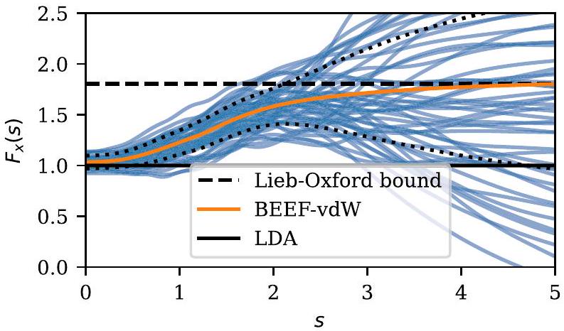
تظهر الشكل 2 مجموعة من عوامل تعزيز التبادلمن دالة BEEF-vdW، حيثهو تدرج الكثافة المخفضة. وقد أدى هذا النهج إلى ظهور عدة دوال، BEEF-vdW،ميتا-بيف (mBEEF) و التي تشمل جميعها تقدير الخطأ ومتاحة بسهولة في GPAW. من خلال واجهة ASE، يمكن للمرء، على سبيل المثال، استخدام مجموعات الأخطاء لتحديد تقديرات الخطأ على النماذج المنفذة بلغة بايثون التي تستخدم محاكاة DFT لتحديد معلماتها. مثال على ذلك هو تطبيق تقديرات الخطأ على علاقات قياس الامتصاص، والميكروكينتيك، واختيار المواد.
أحد المخاطر المرتبطة بالنهج القائم على إنشاء تقديرات الخطأ من مجموعة صغيرة مختارة من دوال XC هو أنه إذا كانت الخاصية المحاكية المعنية موصوفة بشكل سيء من قبل جميع الدوال في المجموعة، فقد تصبح تقديرات الخطأ أيضًا سيئة. قد يكون هذا، على سبيل المثال، هو الحال إذا حاول المرء إنشاء تقدير للخطأ لفراغات النطاق في الأكسيدات أو الروابط فان دير فالز للمواد الماصة على الأسطح استنادًا إلى مجموعة من دوال GGA XC، حيث قد لا تكون أي دالة GGA دقيقة لمحاكاة أي من الخاصيتين.
الشكل 2. مجموعة بايزيان منوظائف حول. الخط الصلب البرتقالي هو عامل تعزيز تبادل BEEF-vdW، بينما الخطوط الزرقاء توضح لـ 50 عينة من المجموعة المولدة عشوائيًا. تحدد الخطوط السوداء المنقطة اضطرابات نموذج التبادل التي تعطي نتائج DFTانحراف معياري بعيدًا عن نتائج BEEF-vdW.
الرابع. ديناميات الأيونات
يمكن استخدام GPAW كحاسبة “صندوق أسود”، حيث يوفر الطاقات والقوى لبرامج أخرى مثل ASE، التي تقوم بعد ذلك بتحسين هندسات الحالة الأساسية ومسارات التفاعل أو تنفيذ الديناميكا الجزيئية. في الواقع، هذه هي مبدأ التصميم الرئيسي وراء GPAW. يجب تنفيذ التطورات المنهجية والتنفيذات العامة التي لا تعتمد مباشرة على الوصول السريع إلى معلومات الهيكل الإلكتروني التفصيلية بشكل خارجي بواسطة GPAW. أدى ذلك إلى أقصى بساطة في كود GPAW نفسه مع السماح أيضًا باستخدام الكود الخارجي واختباره مع أكواد الهيكل الإلكتروني الأخرى والاحتمالات الذرية. مفتاح الكفاءة العالية لمحاكاة GPAW التي تتضمن إزاحات أيونية هو التنفيذ المتنوع للقيود في ASE. هنا، تتوفر العديد من أنواع القيود بسهولة، من الإزالة البسيطة لدرجات الحرية إلى القيود الأكثر غرابة التي تسمح بديناميات الجزيئات الصلبة.قوى الاستعادة التوافقيةحفظ مجموعة الفضاء، وديناميات وحدة الأيونات المدمجة.تتوفر العديد من الخوارزميات لمهام تحسين الهياكل والديناميات الجزيئية المختلفة.
أ. استرخاء الهيكل
عادةً ما يتم تحقيق تحسين الهيكل المحلي في GPAW من خلال استخدام مُحسِّن من ASE. هنا، يتوفر نطاق أوسع من المُحسِّنات القياسية، مثل خوارزميات كوازى-نيوتن بما في ذلك BFGS.و BFGS ذات الذاكرة المحدودة،أو خوارزميات قائمة على الديناميكا النيوتونية مثل MDMin وFIRE.إن حقيقة أن المحسنات قد تم تنفيذها خارجيًا في GPAW توفر فوائد من حيث الإجراءات البسيطة لإعادة تشغيل المحاكاة الطويلة ومراقبة تقاربها. بعض المحسنات منمتاحة أيضًا من خلال حزمة ASE مفتوحة المصدر، التي توفر وسيلة بسيطة لربط أي محسن بتنسيق SciPy مع GPAW. تم تنفيذ المعالجة المسبقة بطريقة سهلة الوصول،الذي غالبًا ما يؤدي إلى تحسينات كبيرة في الأداء.
من بين طرق التحسين الكلاسيكية، تعتبر خوارزميات كوازى-نيوتن غالبًا تنافسية للغاية. هنا، يتم بناء معلومات حول مصفوفة هيسيان أو مصفوفة هيسيان المعكوسة من القوى المحسوبة. في النهاية، يؤدي ذلك إلى نموذج هارموني دقيق لسطح الطاقة المحتملة في محيط الحد الأدنى المحلي. ومع ذلك، يمكن أن تواجه مثل هذه الخوارزميات مشاكل في التعامل مع عدم التناسق في سطح الطاقة المحتملة وأي ضوضاء في محاكاة الهيكل الإلكتروني. غالبًا ما يكون من المنطقي بدلاً من ذلك ملاءمة عملية غاوسية للطاقة والقوى المحسوبة وتقليل الطاقة ضمن هذا النموذج. يتم تنفيذ ذلك كطريقة GPmin في ASE وغالبًا ما تتقارب بسرعة تصل إلى ثلاثة أضعاف أسرع من أفضل المحسنات شبه نيوتن.
ب. مسارات التفاعل والحواجز
تعتبر الحسابات الموثوقة لحواجز الطاقة ذات أهمية كبيرة لتحديد معدل العمليات الذرية. في العديد من الأكواد الكيميائية الكمومية التي تستخدم دوال أساس مركزية دقيقة، يتم تحقيق ذلك باستخدام المشتقات الثانية التحليلية في البحث المباشر عن نقاط السرج من الدرجة الأولى. هذه الطريقة أقل فائدة في أوضاع GPAW المعتمدة على الموجات المستوية أو الشبكات. طريقة الديمريتم تنفيذها في ASE ويمكن استخدامها مع GPAW، ولكن غالبًا ما يرغب المرء في الحصول على نظرة عامة على المسار التفاعلي الكامل لعملية على مقياس ذري للتحقق من أن الحاجز الطاقي الصحيح لعملية ما قد تم تحديده وللحصول على نظرة شاملة على الآلية الذرية. لهذا الغرض، يتم عادةً استخدام طريقة الشريط المرن المدفوع (NEB) من خلال واجهة ASE إلى GPAW. كل من الطريقة الأصليةومجموعة من التحسينات اللاحقة متاحة.يجب اتخاذ عناية خاصة عند اختيار المحسن لخوارزمية NEB، حيث يمكن أن يكون لهذا الاختيار تأثير كبير على معدل التقارب. من أجل تحسين مسار التفاعل، يمكن تحقيق تحسينات كبيرة في الأداء من خلال إجراء التحسين في نموذج تعلم آلي بديل تم ضبطه على سطح الطاقة المحتملة.تم استخدام GPAW لإجراء حسابات NEB على كلا النظامين السطحيينبالإضافة إلى الجزيئات.
ج. تحسين الهيكل العالمي
GPAW متكامل مع أدوات مختلفة للتحسين العالمي للهياكل، والتركيبات، وكذلك أشكال المواد. بعض أدوات التحسين العالمي القابلة للتطبيق بشكل عام المتاحة هي القفز عبر الأحواض،القفز الأدنى،وخوارزميات الجينات.بعض من أقوى مشاكل التحسين العالمي التي تم تناولها باستخدام GPAW تعتمد على استراتيجيات التحسين العالمي المعززة بتعلم الآلة. تم تطبيق هذه الاستراتيجيات، على سبيل المثال، على الأسطح، والعناقيد، والهياكل البلورية بشكل عام.في روتينات تحسين عالمي معززة بتعلم الآلة الأخرى، تم استخدام GPAW لإنشاء قواعد بيانات أولية للأنظمة السطحية والكتلية وللتحقق من النماذج لاحقًا في استراتيجية تستخدم العمليات الغاوسية لتوليد أسطح طاقة محتملة بديلة. ثم تم استكشاف هذه الأسطح باستخدام تقنيات تحسين بايزي، مما حقق تسريعًا مقارنة بالطرق التقليدية بعدة أوامر من حيث الحجم في العثور على الهياكل المثلى للأنظمة قيد البحث.تم تعزيز الطريقة من خلال إدخال أبعاد إضافية (فائقة) عن طريق التداخل بين العناصر الكيميائية، مما يزيد من كفاءة البحث العالمي.تم دمج GPAW مع إطار عمل استراتيجية التطور لتكيف مصفوفة التباين (CMA-ES)، مما يوفر الطاقات والقوى، ويولد بيانات التدريب، ويقيم هياكل المرشحين لـ CMA-ES.
د. الديناميات الجزيئية و QM/MM
يمكن إجراء وتحليل الديناميات الجزيئية من البداية (MD) من خلال واجهة ASE إلى GPAW. يشمل ذلك المحاكاة القياسية مثل محاكاة ثابتة NVE، ثابتة NVT، وثابتة NPT. هناك إمكانية الوصول إلى، على سبيل المثال، ديناميات لانجفين، أندرسن، نوز-هوفر، وبيرندسن. بسبب خارجي الديناميات، يصبح تطوير خوارزميات جديدة وأدوات تحليل أمرًا سهلاً. بعض الأمثلة على استخدام GPAW تشمل دراسات MD من البداية التي استكشفت الهيكل السائل للماء وواجهة الماء/ الكهروكيميائية.
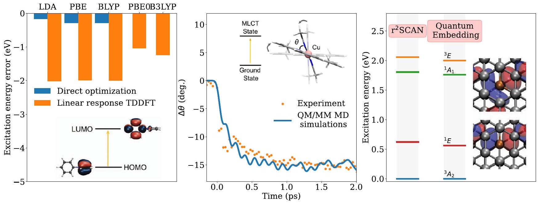
علاوة على ذلك، فإن GPAW قادر على العمل مع مصطلحات الجهد الكهروستاتيكي الخارجي من قيم وشواغل الشحنات النقطية المقدمة من المستخدم، مما يمكّن من محاكاة الديناميات الكمية (QM)/الديناميات الجزيئية (MM). نظرًا لأن GPAW مصمم منذ البداية حول عمليات الشبكة عالية الكفاءة، فإن العبء الحسابي لتقييم هذا الجهد وكذلك القوى الناتجة على الشحنات النقطية MM من كثافة QM يبقى منخفضًا. كان GPAW مركزيًا في مجموعة من الدراسات حول ديناميات الأيونات في المحلول، سواء في حالة التوازن أو خارجه. من خلال استخدام وظيفة الديناميات الجزيئية في ASE، قام الباحثون بإجراء محاكاة MD QM/MM لتكوين الروابط في حالة الإثارة في أنظمة نموذج المحفز الضوئي ونقل الإلكترون، بالإضافة إلى الديناميات التوافقية المرتبطة بالمذاب والمذيب في أنظمة المحفزات الضوئية. العمل على تضمين QM/MM القابل للاستقطاب داخل GPAW جارٍ.
V. المغناطيسية والدوران
تستخدم العديد من التطبيقات التكنولوجية المهمة النظام المغناطيسي أو التلاعب بالدوران في المواد. يحتوي GPAW على مجموعة واسعة من الوظائف التي تسهل تحليل الخصائص المغناطيسية. يشمل ذلك الحسابات مع الدوران غير المتوازي، وإدراج المجالات المغناطيسية الخارجية، وترابط الدوران-المدار، وحسابات الدوران الحلزونية ضمن نظرية بلوتش العامة. يتم وصف تنفيذ هذه الميزات أدناه، بينما يتم وصف طرق إضافية لحساب الإثارات المغناطيسية في القسم VI D.
أ. ترابط الدوران-المدار
عادةً ما يهيمن ترابط الدوران-المدار تمامًا على المناطق القريبة من النوى، حيث يصبح الجهد الكهروستاتيكي قويًا. ضمن كرة تعزيز PAW للذرة ، يتم إعطاء مكون الدوران- من المدار بواسطة
بافتراض وجود جهد كروي متماثل، يتم كتابة هاملتونيان الدوران-المدار للذرة على النحو التالي
حيث هو الجهد الكهروستاتيكي الشعاعي للذرة . نقوم بتقييم كجزء كروي من جهد XC و هارتري من التوسع المحلي للكثافة المعطاة بواسطة المعادلة (11). نظرًا لأن الموجات الجزئية هي حالات ذاتية لهاملتونيان النسبي القياسي، فإنها مستقلة عن الدوران، ومن السهل تقييم تأثير عليها.
يمكن حساب الطاقات الذاتية بدقة في معالجة غير ذاتية لتفاعل الدوران-المدار ويمكن الحصول عليها من خلال تشخيص الهاملتونيان الكامل على أساس المدارات النسبية القياسية،
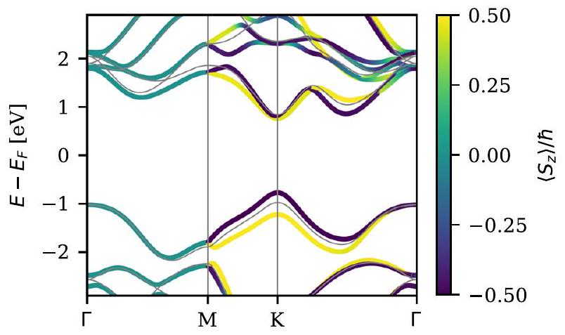
هنا، و تمثل الطاقات الذاتية النسبية القياسية والحالات الذاتية، على التوالي. يشكل هذا خطوة معالجة سريعة لأي حساب نسبي قياسي ويتطلب فقط تداخلات المشروع . يجب ملاحظة أن هذا النهج يتطلب من حيث المبدأ التقارب فيما يتعلق بعدد الحالات النسبية القياسية المضمنة في الأساس، ولكن القيم الذاتية عادة ما تتقارب بسرعة نسبية مع الأساس. في الشكل 3، نعرض هيكل الشريط ل طبقة أحادية تم الحصول عليها من PBE مع ترابط الدوران-المدار غير الذاتي. تقدم ذرات W ترابطًا قويًا للدوران-المدار في هذه المادة، وينقسم نطاق التكافؤ بمقدار 0.45 eV عند نقطة K. يتم الاحتفاظ بتدهور الدوران على طول خط -M، الذي يبقى ثابتًا بواسطة تناظرات مرآة غير متبادلة.
بالنسبة للمواد المغناطيسية، فإن المعالجة غير الذاتية لترابط الدوران-المدار مريحة لتقييم الأنيسوتروبي المغناطيسي. ينص نظرية القوة المغناطيسية على أن تدوير العزوم المغناطيسية بعيدًا عن تكوين الحالة الأرضية ينتج عنه مساهمة في الطاقة، والتي يتم تقريبها بشكل جيد من خلال التغيير في قيم كوهين-شام الذاتية. يمكن الحصول على التغيير في الطاقة لتوجه معين لكثافة المغناطيسية على النحو التالي
حيث هي القيم الذاتية التي تم الحصول عليها من تشخيص المعادلة (29) مع تدوير الدوران في اتجاه محدد بواسطة الزوايا و هي أرقام الشغل المرتبطة. يتوافق هذا مع تدوير المجال المغناطيسي xc (المحدد أدناه)، مما سيؤدي إلى قيم ذاتية مختلفة عند تضمين ترابط الدوران-المدار. في المغناطيسات ثنائية الأبعاد، تعتبر الأنيسوتروبي المحور السهل حاسمة للنظام المغناطيسي، والمعادلة (30) تنطبق بسهولة على حسابات الخصائص المغناطيسية عالية الإنتاجية.
الشكل 3. هيكل الشريط ل طبقة أحادية تم الحصول عليها من PBE مع ترابط الدوران-المدار غير الذاتي. تشير الألوان إلى القيمة المتوقعة لـ لكل حالة. تظهر الخطوط الرمادية هيكل الشريط بدون ترابط الدوران-المدار.
ب. المغناطيسية غير المتوازية الذاتية
تم تطوير إطار كوهين-شام لمعالجة المغناطيسية غير المتوازية بواسطة بارث وهدين ويتضمن مصفوفة كثافة الدوران
كمتغير أساسي. ثم يتم إعطاء الكثافة الإلكترونية والمغناطيسية بواسطة و ، على التوالي. يكتسب جهد XC أربعة مكونات، وهي المشتقات الوظيفية لطاقة XC بالنسبة لمصفوفة الكثافة ويمكن تمثيلها كمصفوفة تعمل على حالات كوهين-شام الدورانية. يمكن التعبير عنها من حيث الكثافة والمغناطيسية، مما يؤدي إلى الجزء XC من هاملتونيان كوهين-شام
حيث يتم إعطاء الجهد القياسي والمجال المغناطيسي XC بواسطة
في GPAW، يتم تنفيذ المعالجة الذاتية للدوران غير المتوازي ضمن LDA، حيث يتم تقريب كالتالي
هنا، هو المقدار، و هو اتجاه المغناطيسية. تعاني تعميم المعادلة (34) إلى GGAs من مشاكل رسمية وكذلك عددية، والحل الذاتي لمعادلات كوهين-شام غير المتوازية مقيد حاليًا بـ LDA. يجب التأكيد على أن صيغة PAW تسمح بمعالجة غير متوازية بالكامل لا تعتمد على التوازي داخل الذرة، والذي غالبًا ما يتم فرضه في حزم هيكل إلكتروني أخرى.
يمكن تضمين ترابط الدوران-المدار عن طريق إضافة المعادلة (28) إلى هاملتونيان كوهين-شام، وهذا يشكل إطارًا ذاتيًا بالكامل لحسابات الدوران-المدار ضمن LDA.
ج. المغناطيسية المدارية
تشمل الطرق الحالية لتحديد المغناطيسية المدارية لمادة ما إما النظرية الحديثة، أي، صيغة مرحلة بيري، أو تقريب مركز الذرة (ACA)، حيث يتم تقييد المساهمات في القيمة المتوقعة لمشغل الزخم الزاوي ضمن كرات مافين-تين (MT) المركزية بالذرة مع أنصاف أقطار محددة. يسمح صياغة PAW للدوال الموجية بتقريب مشابه لـ MT-ACA، حيث يُفترض أن يساهم فقط توسيع PAW للدوال الموجية بشكل كبير في القيمة المتوقعة للزخم الزاوي. يمكن بعد ذلك حساب العزوم المغناطيسية المدارية من خلال
حيث هي عناصر مصفوفة كثافة الذرة كما هو محدد في المعادلة (9)، هي الموجات الجزئية الكاملة للذرة ، و هو مشغل الزخم الزاوي.
الجدول II. القيم المحسوبة والمقاسة للمغناطيسية المدارية بوحدات من لكل ذرة.
المحور السهل البلوري
bcc-Fe [001]
fcc-Ni [111]
fcc-Co [111]
hср-Со [001]
PAW-ACA
0.0611
0.0546
0.0845
0.0886
MT-ACA
0.0433
0.0511
0.0634
0.0868
النظرية الحديثة
0.0658
0.0519
0.0756
0.0957
التجربة
0.081
0.053
0.120
0.133
نلاحظ أن هذه المعادلة لا تتطلب أنصاف أقطار للمدخلات الذرية للمغناطيسية المدارية؛ بدلاً من ذلك، يتم تضمين الموجة الجزئية الكاملة، على الرغم من أن التوسع الذري الكامل هو دقيق فقط داخل كرات PAW. بالإضافة إلى ذلك، يعني ذلك أنه يجب استبعاد الموجات الجزئية غير المحدودة، أي، غير القابلة للتطبيع، في المعادلة (35).
شرط أساسي لوجود مغنطة مدارية غير صفرية هو كسر تناظر عكس الزمن، كما يتم تمثيله بواسطة هاملتوني معقد ليس معادلاً وحدوياً لنظيره الحقيقي. عملياً، يعني ذلك أن وجود مغنطة مدارية محدودة يتطلب ترتيباً مغناطيسياً وإما تضمين تفاعل الدوران-المدار أو أنسجة دوران غير مستوية. في GPAW، يمكن تضمين تفاعل الدوران-المدار إما بشكل ذاتي التناسق في حساب غير متوازي أو كخطوة معالجة لاحقة غير ذاتية التناسق بعد حساب متوازي. تم حساب المغنطة المدارية باستخدام المعادلة (35) للمواد المغناطيسية البسيطة مثل bcc-Fe وfcc-Ni وfcc-Co وhcp-Co، حيث تم تضمين تفاعل الدوران-المدار بشكل غير ذاتي التناسق. تظهر نتائج PAW-ACA في الجدول II جنباً إلى جنب مع نتائج MT-ACA ونتائج النظرية الحديثة وقياسات من التجارب، مما يوضح بشكل رئيسي أن PAW-ACA يمكن أن يكون تحسيناً على MT-ACA وثانياً أن هناك توافقاً جيداً بين PAW-ACA والنظرية الحديثة لهذه الأنظمة.
د. مجال مغناطيسي ثابت
ترابط لحظات المغناطيسية للدوران الإلكتروني مع حقل مغناطيسي خارجي ثابتيمكن تضمينه من خلال إضافة حد زيمان في هاملتونيان كوهين-شام.
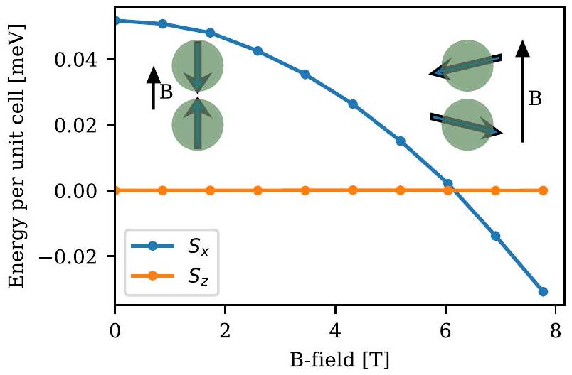
كمثال، يمكننا اعتبار انتقال دوران الفلّوب فيالحالة الأرضية مضادة للمغناطيسية مع أنيسوتروبي ضعيف يفضل محاذاة الدورانات مع-المحور، وإذا تم تطبيق مجال مغناطيسي على طول-الاتجاه، يصبح من المفضل محاذاة الدورانات على اتجاه عمودي (مع مكون فيرومغناطيسي صغير) عند المجال الحرج حيث تتغلب طاقة زيمان على الأنيسوتروبي. هذا بوضوح تأثير دوران-مدار، ويجب إجراء الحسابات في إطار غير متوازي بالكامل مع اقتران دوران-مدار ذاتي الاتساق. في الشكل 4، نعرض طاقة المحاذاتين للدوران كدالة للمجال المغناطيسي الخارجي الذي تم الحصول عليه مع. تتغير تكوين الطاقة الدنيا من إلىالتوافق عند 6 تسلا، أي أن العزم المغزلي ينقلب عند هذا المجال الحرج. هذا يتوافق بشكل ممتاز مع القيمة التجريبية في المرجع 199. ومع ذلك، فإن المجال الحرج يعتمد بشكل قوي على القيمة المختارة لـويزداد بمقدار الضعف
الشكل 4. انتقال دوران الفلّوب فيتم رسم محاذاة الدورانات بالنسبة للمجال المغناطيسي لأحجام صغيرة وكبيرة من المجال. تم تضخيم الميل (المكون الفيرومغناطيسي الصغير بعد انقلاب الدوران) لأغراض التوضيح. الميل الفعلي هو تقريبًا.
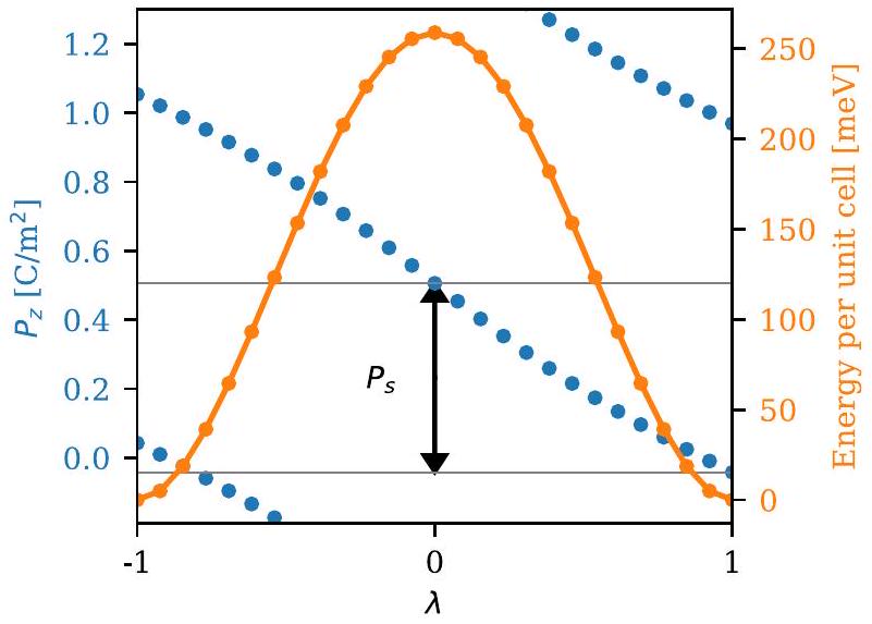
في غيابيمكن قراءة الأنيسوتروبي المغناطيسي (لكل وحدة خلوية) من فرق الطاقة عند.
دوامات الدوران
غالبًا ما تكون البنية المغناطيسية في الحالة الأساسية للمغناطيسات المحبطة و/أو الحلزونية غير متوازية وقد تكون غير متوافقة مع وحدة الخلية الكيميائية. في نموذج هايزنبرغ الكلاسيكي المتساوي، يتم دائمًا تقليل الطاقة بواسطة لولب دوران مستو.يمكن تقييم طاقة لولب الدوران العام في المستوى بكفاءة داخل وحدة الخلية الكيميائية باستخدام نظرية بلخ العامة (GBT).في تنفيذ GBT لـ GPAW،لا توجد قيود على التوازي بين الذرات، وبالتالي، فإنه يشفر دوران كثافة المغنطة الإلكترونية بالكامل بزاويةعند ترجمة متجه الشبكةيمكن بعد ذلك حل معادلات كون-شام بشكل ذاتي الاتساق لزاوية موجية ثابتة،
باستخدام الجزء الدوري فقط من المدارات العامة لبلاخ،، حيث يشير إلى دوران الدوران حول-محور:
الهاميلتوني العام لبلاخ بدون اقتران الدوران-المدار يُعطى بواسطة
وبمجرد حل المعادلة (37) بشكل ذاتي الاتساق لعدد معينيتم تقييم طاقة اللولب الدوراني المقابل كما هو معتاد،.
استخدام وظيفة GPAW لحساب طاقة الحلزونات المغناطيسية كدالة لـيمكن بعد ذلك البحث عن متجه الموجة في الحالة الأساسيةالذي يقلل من الطاقة. في الشكل 5، نوضح أن الطبقة الأحاديةيمتلك حالة أرضية لولبية ذات دوران غير متناسب
الشكل 5. طيف لفة الدوران LSDA لـطبقة أحادية (هيكل مأخوذ من C2DB)الحالة الأساسية لها متجه موجي غير متناسبيعرض العزم المغناطيسي تقلبات طولية ضعيفة فقط، وتبقى فجوة الطاقة محدودة لجميع متجهات الموجة.، مما يشير إلى أن وصف نموذج هايزنبرغ للمادة سيكون مناسبًا. يوضح الشكل الفرعي تصحيح العزم الزاوي لطاقة الحلزونات المغناطيسية (بـ meV) كدالة للمتجه العادي.للولب المغزلي السطحي.يتم تصويره من حيث إسقاطه الاستريوغرافي في نصف الكرة العلوي فوق مستوى الطبقة الأحادية. ويظهر أن المستوى الحلزوني عمودي على Q ومائل قليلاً بالنسبة للاتجاه خارج المستوى.
وأن العزم المغناطيسي المحلي على ذرة النيكل يعتمد فقط بشكل ضعيف على متجه الموجة.
علاوة على ذلك، يمكن الحصول على اتجاه لولب دوران الحالة الأساسية من خلال تضمين اقتران الدوران-المدار بشكل غير ذاتي الاتساق في تقريب الدوران-المدار المُسقَط. وابحث عن الاتجاه الذي يقلل من الطاقة. متجه الترتيب والمتجه العموديلذا تشكل الطائرة الحلزونية مواصفة كاملة للحالة المغناطيسية الأساسية ضمن فئة الأحادية-الدول. المتجه العمودي له أهمية خاصة حيث إن الحلزونات المغناطيسية قد تؤدي إلى كسر تلقائي لتماثل البلورة، والمتجه العمودي يحدد إلى حد كبير اتجاه الاستقطاب التلقائي الناتج عن المغناطيسية.في الشكل 5، نوضح أنعمودي على متجه الموجةفي الطبقة الأحاديةالحالة الأساسية، التي تت correspond إلى لولب دوران دوري.
VI. وظائف الاستجابة والإثارات
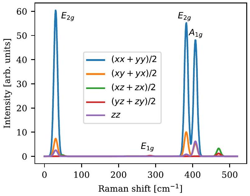
تعتبر دوال الاستجابة الخطية الأساس في فيزياء المادة المكثفة. تشمل تطبيقاتها وصف الشاشات العازلة، وطيف فقدان الطاقة البصرية والإلكترونية، والإثارات متعددة الجسيمات، وطاقة الارتباط في الحالة الأساسية. في هذا القسم، نصف الطرق المتاحة في GPAW لحساب دوال الاستجابة الإلكترونية بالإضافة إلى هياكل النطاقات الكوانتية لجسيمات GW والإثارات البصرية من معادلة بيته-سالبيتر (BSE). بالإضافة إلى دالة الاستجابة الإلكترونية، يمكن لـ GPAW أيضًا حساب القابلية المغناطيسية العرضية، التي تحتوي على معلومات حول الإثارات المغناطيسية، مثل الماجنون، ويمكن استخدامها لاشتقاق معلمات لنماذج دوران هايزنبرغ الكلاسيكية وتقدير درجات حرارة الانتقال المغناطيسي. أخيرًا، نقدم طرقًا لحساب أطياف رامان للمواد الصلبة وموترات الاستجابة البصرية التربيعية لوصف توليد التوافقيات الثانية وتأثير بوكيلز الكهروضوئي.
أ. نظرية الكثافة الزمنية ذات الاستجابة الخطية
بالترتيب الخطي، التغير في كثافة الإلكترونات الناتج عن جهد خارجي (عدد) يعتمد على الزمنتحكمه القابلية الإلكترونية،،
الاستجابة تُعطى بنفسها بواسطة معادلة كوبو
حيث يتم أخذ قيمة التوقع بالنسبة للحالة الأساسية عند درجة حرارة صفر ويتم صياغة مشغلات الكثافة في صورة التفاعل.
في نظام كوهين-شام غير المتفاعل، يمكن تقييم القابلية بشكل صريح من المدارات كوهين-شام، والقيم الذاتية، والاحتلالات.
استنادًا إلى قابلية كوهين-شام،يمكن حساب قابلية الجسم المتعدد من خلال معادلة شبيهة بمعادلة دايسون
هنا، يتم احتساب التفاعلات الإلكترونية من خلال نواة هارتري-إكس سي، التي تُعرّف من حيث الجهود الفعالة لنظرية الكثافة الزمنية (TDDFT).
أين هو تفاعل كولومب يتم تعريف نواة XC على أنها
في حسابات الاستجابة الخطية النموذجية (LR-TDDFT)، يتم إما تجاهل جزء تبادل-الارتباط من النواة [مما يؤدي إلى تقريب الطور العشوائي (RPA)] أو يتم تقريبه من خلال تقريب الكثافة المحلية الأديباتيكية (ALDA).
أينيمثل طاقة XC لكل إلكترون في الغاز الإلكتروني المتجانس ذو الكثافةإن ALDA في الواقع مقيدة إلى حد ما، حيث إنها تضمن فقط وصفًا صحيحًا للنواة للمعادن في حد الطول الموجي الطويل. وهذا يعني أنها لا تستطيع حساب الإثارات في الأنظمة الممتدة، وعلاوة على ذلك، يؤدي ذلك إلى ثقب XC متباين. يمكن حل المشكلة الأخيرة من خلال إعادة تنظيم بسيطة لـ ALDA التي تنظم ثقب XC العلوي وتحسن بشكل كبير وصف التفاعلات المحلية مقارنةً بـ ALDA (و RPA).
1. التنفيذ للأنظمة الدورية
في الأنظمة البلورية، تكون القابلية دورية بالنسبة للترجمات على شبكة برافيس.. وبالتالي، يمكن تحويل القابلية إلى تحويل فورييه وفقًا لـ
ترجمة معادلة دايسون (43) إلى معادلة مصفوفة للموجات المستوية، والتي تكون قطرية في متجه الموجةويمكن عكسه عدديًا.
من خلال استخدام تمثيل الموجة المسطحة، تصبح جوهر التنفيذ بعد ذلك حساب كثافات الأزواج في الفضاء المعكوس.
وإجراء تحويل فورييه لنواة XC
من المهم أن كلاهما يمكن تقييمه عن طريق إضافة تصحيح PAW إلى الكمية الزائفة المماثلة، والتي يمكن تقييمها بدورها بواسطة تحويل فورييه السريع (FFT). تم الإبلاغ عن تفاصيل التنفيذ المتعلقة بذلك في المراجع 36 و 43.
مساهمة هارتري في النواة (44) تُعطى ببساطة من خلال التفاعل الكهروستاتيكي البسيط (المعطى هنا بوحدات ذرية).
ويمكن تقييمه تحليليًا عندما有限的。然而,在光学极限中,يتباعد المكون، ويجب أن تكون حذرًا عند عكس معادلة دايسون (43). في GPAW، يتم التعامل مع ذلك من خلال توسيع كثافات الأزواج ضمن-نظرية الاضطراب,
في التوسع، يتم إلغاء مصطلح كولومب المتباعد تمامًا بواسطة-اعتماد كثافات الزوج بحيث يكون الناتجيبقى محدودًا. لمزيد من التفاصيل، انظر المرجع 36.
2. التمثيل الطيفي
يقدم GPAW طريقتين مختلفتين للتعامل مع الاعتماد الترددي لحساسية كوهين-شام (42). واحدة هي تقييم التعبير بشكل صريح للترددات المعنية. هذه الطريقة مفيدة إذا كان الشخص مهتمًا بعدد قليل من الترددات المحددة. الأخرى هي تقييم الدالة الطيفية المرتبطة.
التي يمكن الحصول على القابلية من خلالها عبر تحويل هيلبرت،
للتقارب في تحويل هيلبرت، يتم تقييم الدالة الطيفية على شبكة تردد غير خطية تمتد عبر نطاق اختلافات الطاقة الذاتية المدرجة في المعادلة (52). على الرغم من أن الحساب يصبح أكثر استهلاكًا للذاكرة نتيجة لذلك، إلا أنه عادة ما يكون أسرع في الحساب.عبر دالتها الطيفية. علاوة على ذلك، نظرًا لأنيمكن استخدام طريقة الهرم الرباعي لتحسين التقارب بالنسبة لـ-نقاط.
ب. دالة العزل الكهربائي
الجزء الطولي من موتر العزل الكهربائي مرتبط بالاستجابة.كما
من المصفوفة العازلة، يتم إعطاء الدالة العازلة الكلية، بما في ذلك تصحيحات المجال المحلي، بواسطة
من السهل استخراج طيف الامتصاص البصري منه
بالإضافة إلى طيف فقدان طاقة الإلكترون
من الممكن أيضًا تعريف نسخة متماثلة من مصفوفة العازل على أنها
يمكن تقييم القابلية عند مستوى RPA [عن طريق ضبطفي المعادلة (43) إلى الصفر] أو باستخدام أحد نوى XC المطبقة في GPAW مثل ALDA المحلي، أو ALDA المعادلة غير المحلية (rALDA)،أو نواة التمهيد.
التقييميتطلب حسابيًا جهدًا كبيرًا لأنه يتضمن تكاملًا على منطقة بريلوان (BZ) بالإضافة إلى جمع الحالات المأهولة وغير المأهولة.يمكن زيادة تقارب النقاط بشكل كبير باستخدام طريقة الرباعي.على عكس تكامل النقاط البسيط، حيثالدالة في المعادلة (52) يتم استبدالها بلورنتزيان مموه، بينما تستخدم طريقة الرباعي الاستيفاء الخطي للقيم الذاتية وعناصر المصفوفة.
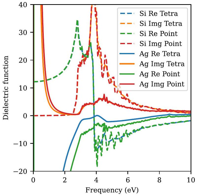
في الشكل 6، نقارن بين الدالة العازلة المحسوبة باستخدام طريقتي التكامل المختلفتين لحالتين نموذجيين: (الموصل) السيليكون و(المعدن) الفضة. نظرًا لأن السيليكون موصل، فلا توجد إثارات ذات طاقة منخفضة، وبالتالي فإن الجزء التخيلي من الدالة العازلة يساوي صفرًا، بينما الجزء الحقيقي مستوٍ عند الترددات المنخفضة. تكامل النقطة والهرم الرباعي
الشكل 6. الأجزاء الحقيقية والتخيلية من دالة العزل الكهربائي للفضة (صلب) والسيليكون (منقط) باستخدام طرق التكامل الهرمي والنقطي.
التكامل يعطي نفس القيمة لـلكن تكامل الهرم الرباعي يتجنب الاهتزازات غير الفيزيائية لـ عند الترددات الأعلى التي تظهرها التكامل النقطي بسبب النهاية -نقاط أخذ العينات. بالنسبة للمعادن، تقارب النقطة أبطأ حتى، وبالتالي فإن الفرق بين تكامل النقطة وتكامل الهرم الرباعي يكون أكثر وضوحًا بالنسبة لـ Ag. من خلال زيادةستقترب نتائج تكامل النقاط في النهاية من النتائج التي تم الحصول عليها باستخدام طريقة الهرم الرباعي، ولكن بتكلفة حسابية أعلى بكثير.
1. الفحص في الأنظمة ذات الأبعاد المنخفضة
في بلورة ثلاثية الأبعاد (3D)، ترتبط الدالة العزلية الكلية بالقطبية الكلية.المادة كـ
منذ يتعلق بالمتوسط المجهري للإمكانات المستحثة، وسيعتمد على وحدة الخلية في الأنظمة ذات الأبعاد المنخفضة ويميل إلى الوحدة عند زيادة الخلية في الاتجاه غير الدوري. على النقيض من ذلك، من السهل تعميم تعريف الاستقطابية بحيث يقيس العزم الثنائي المستحث لكل طول أو مساحة بدلاً من الحجم. الاستقطابية ذات الأبعاد – تُعرف بذلك على أنها، حيث هو حجم الخلية مع الاتجاهات الدورية المستبعدة. على سبيل المثال، بالنسبة لمادة ثنائية الأبعاد،هو ببساطة طول وحدة الخلية في الاتجاه غير الدوري. لتحسين التقارب فيما يتعلق بحجم وحدة الخلية، يتم تقليم نواة كولوم باستخدام طريقة الفضاء العكسي التي تم تقديمها في المرجع 208. وهذا يمكّن من حسابات فعالة لخصائص العزل للمواد ذات الأبعاد المنخفضة.هذا، مع ذلك، يعني أن القابلية للاستقطاب لا يمكن تقييمها مباشرة من الثابت العازل (الذي هو واحد فقط)، ولكن يمكن الحصول عليها مباشرة من القابلية كما هو
ث. نظرية التقلبات والانحلال في الاتصال الأديباتيكي
نظرية التقلبات والانحلال في الاتصال الأديباتي (ACFDT) هي نهج واعد للغاية لبناء دوال الارتباط الدقيقة ذات الخصائص غير المحلية. على عكس دوال XC العادية، فإن دوال الارتباط ACFDT لا تعتمد على إلغاء الأخطاء بين التبادل والارتباط. بدلاً من ذلك، توفر ACFDT نظرية دقيقة لطاقة الارتباط الإلكتروني.من حيث القابلية الإلكترونية التفاعلية، التي يمكن دمجها مع التبادل الدقيق،
يمكن التعبير عن دالة الاستجابة من حيث دالة استجابة كوهين-شام ونواة التبادل-الارتباط.
يمكن اشتقاق تقريب الطور العشوائي (RPA) من ACFDT إذا كان نواة XCيتم تجاهله. تتمتع RPA بقدرة على التقاط تأثيرات الترابط غير المحلية وتوفر دقة عالية عبر أنواع الروابط المختلفة، بما في ذلك تفاعلات فان der Waals.
يمكن أيضًا دمج نوى التبادل-الارتباط البسيطة في دالة الاستجابة، مثل نواة LDA الأديباتية (ALDA). ومع ذلك، فإن محلية النوى الأديباتية تؤدي إلى خصائص متباينة لدالة الارتباط الزوجي.يمكن التغلب على هذه المشكلة من خلال نظام إعادة التعيين (r).الذي تم تنفيذه في GPAW كـ rALDA. توفر هذه الفئة من النوى المعاد توصيلها وصفًا أفضل بكثير للتفاعلات القصيرة المدى، وبالتالي، تعطي أيضًا طاقات ارتباط إجمالية دقيقة للغاية.
د. الاستجابة المغناطيسية
يمكن تعميم إطار LR-TDDFT الموصوف في القسم VI A ليشمل درجات حرية الدوران.باستخدام كثافة المكونات الأربعة كمتغير أساسي، (حيث يمكن للمرء تعريف موتر القابلية ذو الأربعة مكونات،
بطريقة مشابهة للمعادلة (43)، الجسم المتعدديمكن حسابه من موتر القابلية المقابل لنظام كوهين-شام،. في الحالة الأكثر عمومية، معادلة دايسون لـهي معادلة مصفوفة في و المؤشرات، التي تربط بشكل صريح بين شحنات الدوران ودرجات الحرية. ومع ذلك، بالنسبة للأنظمة المغناطيسية المتوازية، فإن المكونات العرضية للحساسية تنفصل عن البقية في غياب اقتران الدوران-المدار.
1. الحساسية المغناطيسية العرضية
من خلال اعتبار الدورانات مستقطبة على طول -الاتجاه، يمكن التعبير عن الحساسية المغناطيسية العرضية للأنظمة غير النسبية المتوازية من حيث مشغلات كثافة رفع وخفض الدوران و . في ALDA، تصبح معادلة دايسون لـ بعد ذلك معادلة عددية،
حيث يتم إعطاء نواة XC العرضية بواسطة . الحساسية و تعرف نفسها من خلال صيغة كوبو (63)، حيث يمكن تقييم الأخيرة بشكل صريح في تشابه كامل مع المعادلة (42)،
في GPAW، يتم حساب الحساسية المغناطيسية العرضية باستخدام أساس الموجة المسطحة كما هو موضح في القسم VI A 1، مع الاستثناء الملحوظ أنه لا حاجة لرعاية خاصة لمعالجة الحد البصري حيث لا تلعب نواة هارتري أي دور في معادلة دايسون (64). من حيث التمثيل الزمني، في وقت كتابة هذا النص، من الممكن فقط إجراء تقييم حرفي للمعادلة (65) عند الترددات المعنية. بالنسبة للمعادن، يعني هذا أن يجب أن تترك كمعامل توسيع محدود، والذي يجب اختياره بعناية اعتمادًا على أخذ عينات النقاط (انظر المرجع 43).
2. طيف الإثارات المغناطيسية العرضية
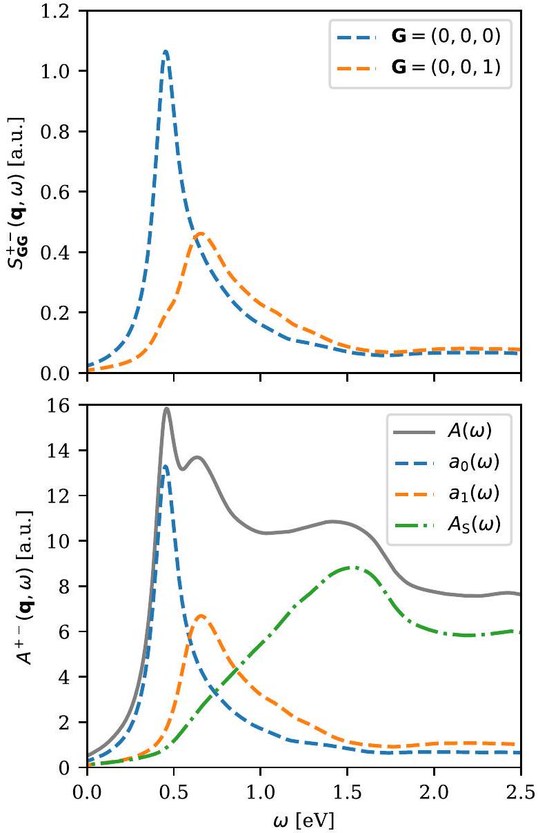
استنادًا إلى الحساسية المغناطيسية العرضية، يمكن للمرء حساب الدالة الطيفية المقابلة
التي تحكم مباشرة فقدان الطاقة في مغناطيس متوازي يتعلق بالتغيرات المستحثة في إسقاط الدوران على طول -محور . على وجه الخصوص، يمكن للمرء تحليل الطيف إلى مساهمات من إثارات الدوران الغالبة والأقلية، ، أي، إلى دوال طيفية للحالات المثارة حيث تم خفض أو رفع بوحدة واحدة من الزخم الزاوي للدوران، على التوالي،
هنا، يكرر حالات النظام الذاتية، مع تشير إلى الحالة الأساسية.
بالنسبة للأنظمة المغناطيسية المتوازية، يتكون الطيف من نوعين من الإثارات: إثارات موجات الدوران الجماعية (المعروفة باسم الماجنون) وإثارات في استمرارية ستونر (أزواج الإلكترون-الثقب ذات الدوران المعاكس). نظرًا لأن GPAW تستخدم تمثيل الموجة المسطحة للطيف، ، يمكن للمرء مقارنة الناتج الحسابي مباشرة مع مقطع تشتت النيوترون غير المرن المقاس في التجارب.
على وجه الخصوص، يمكن للمرء استخراج انتشار الماجنون مباشرة من خلال تحديد موضع القمم في القطر الطيفي (انظر الشكل 7). بهذه الطريقة، يسمح GPAW للمستخدم بدراسة ظواهر الماجنون المختلفة في الأنظمة المغناطيسية من ترتيب متوازي عشوائي، مثل تأثيرات الانتشار غير التحليلية في الفيرومغناطيسات المتنقلة، الانتقالات الطورية المغناطيسية المدفوعة بالترابط، وظهور أوضاع جماعية متميزة داخل استمرارية ستونر لمغناطيس مضاد.
بالإضافة إلى ذلك، يمكن للمرء تحليل الطيف بشكل أكثر تعقيدًا من خلال استخراج الأوضاع الذاتية الغالبة والأقلية من كقيم ذاتية إيجابية وسلبية، على التوالي. على عكس تحليل القطر الموجي المسطح، يجعل هذا من الممكن تمامًا
الشكل 7. طيف الإثارات المغناطيسية العرضية لمغناطيس الفيرومغناطيس hcp-Co تم تقييمه عند . تم حساب الطيف باستخدام ثمانية نطاقات فارغة لكل ذرة، وقطع موجة مسطحة قدره -نقطة شبكة، وتوسيع طيفي قدره . في اللوحة العليا، يتم تصوير القطر الطيفي للمناطق البريل الأولى والثانية خارج المستوى السداسي، والتي يمكن من خلالها استخراج ترددات الماجنون الصوتية والبصرية على التوالي. في اللوحة السفلية، يتم عرض طيف الإثارات الغالبة. يتم حساب الوزن الطيفي الكامل كمجموع لجميع القيم الذاتية الإيجابية لـ ، يتم الحصول على أشكال خطوط الأوضاع الصوتية والبصرية و من خلال أكبر قيمتين ذاتيتين (والتي تكون أكبر بكثير من البقية)، ويتم استخراج طيف ستونر كفرق .
افصل تحليل كل شكل خط ماجن فردي وكذلك استمرارية ستونر متعددة الجسيمات (انظر الشكل 7).
3. الاستجابة الخطية MFT
لا يمكن استخدام الحساسية المغناطيسية العرضية فقط لدراسة الإثارات المغناطيسية بمعنى حرفي، ولكن يمكن أيضًا استخدامها لرسم درجات حرية الدوران إلى نموذج هايزنبرغ الكلاسيكي،
حيث و تشير إلى مؤشرات شبكة برافيس والشبكة المغناطيسية، على التوالي، هو اتجاه استقطاب الدوران للموقع المغناطيسي المعطى. استنادًا إلى نظرية القوة المغناطيسية (MFT)، يمكن حساب معلمات تبادل هايزنبرغ LSDA من الجزء التفاعلي من الحساسية الثابتة لكوهين-شام و المجال المغناطيسي الفعال ، باستخدام صيغة MFT المعروفة جيدًا لـ
هنا، تشير إلى حجم الموقع، الذي يحدد بشكل فعال نموذج هايزنبرغ (68).
باستخدام تمثيل GPAW للموجة المسطحة لـ ، يمكن للمرء حساب معلمات التبادل المحولة فورييه للشبكة مباشرة،
حيث يتم كتابة الجانب الأيمن من المعادلة الثانية في أساس الموجة المسطحة و تشير إلى نواة موقع الشبكة،
نظرًا لعدم وجود تعريف مسبق لأحجام المواقع المغناطيسية، توفر GPAW وظيفة لحساب معلمات التبادل استنادًا إلى تكوينات مواقع كروية، أسطوانية، و/أو متوازي المستطيلات ذات الأحجام المتغيرة.
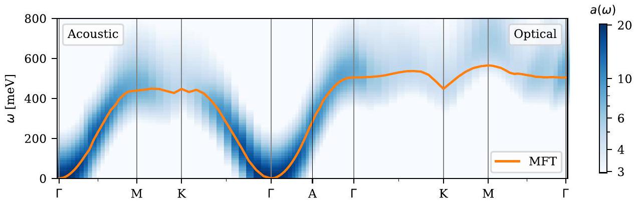
عند حساب معلمات التبادل ، من السهل حساب انتشار الماجنون ضمن نموذج هايزنبرغ الكلاسيكي باستخدام نظرية موجة الدوران الخطية وتقدير الكميات الحرارية مثل درجة حرارة كوري (انظر، على سبيل المثال، المرجع 42). في الشكل 8، يتم مقارنة انتشار ماغنون MFT لـ hcp-Co مع طيف ماغنون الغالب المحسوب ضمن LR-TDDFT. بالنسبة لـ Co، فإن الاثنين متوافقان تمامًا باستثناء انتشار وضع الماجنون البصري على طول المسار عالي التناظر، حيث يقلل MFT من تردد الماجنون ويتجاهل الهيكل الدقيق للطيف. يظهر الهيكل الدقيق لطيف ALDA بسبب التداخل بين وضع الماجنون واستمرارية ستونر. وهذا يؤدي إلى ما يسمى بظواهر كوهين (نقاط غير تحليلية في انتشار الماجنون)، والتي هي علامة مميزة للمغناطيسية الإلكترونية المتنقلة. نظرًا لأن التنقل يتم تجاهله إلى حد كبير في نموذج الدوران المحلي مثل (68)، لا يمكن للمرء عمومًا توقع التقاط مثل هذه التأثيرات.
الشكل 8. طيف الماجنون لمغناطيس الفيرومغناطيس hcp-Co المحسوب باستخدام ALDA LR-TDDFT (مبين كخريطة حرارية) مقارنة مع انتشار موجة الدوران لنموذج MFT لليختنشتاين. يتم عرض وضع الماجنون الصوتي إلى يسار نقطة A، بينما يتم عرض وضع الماجنون البصري إلى اليمين. لاحظ أن الوضعين متطابقان عند كل من نقاط A و K عالية التناظر. تم إجراء الحسابات باستخدام ثمانية نطاقات فارغة لكل ذرة، وقطع موجة مسطحة قدره 800 eV، وشبكة ( ) -نقطة. تم استخدام قيمة محدودة لـ لتوسيع طيف ALDA. بالنسبة لحسابات MFT، تم حساب الانتشار باستخدام نظرية موجة الدوران الخطية استنادًا إلى نموذج هايزنبرغ لمواقع كروية مغلقة مركزة عند كل من ذرات Co.
E. تقريب GW
يدعم GPAW حسابات الجسيمات الكمية القياسية استنادًا إلى معالجة اضطرابية من الدرجة الأولى لمعادلة QP الخطية
حيث و هما القيم الذاتية لوظائف كوهين-شام، و و هما الجهد المحلي XC والجهد التبادلي غير المحلي، على التوالي. هو (الجزء الديناميكي من) الطاقة الذاتية GW التي يتم أخذ اعتمادها على التردد في الاعتبار من الدرجة الأولى بواسطة عامل إعادة التشكيل . كما هو موضح بواسطة المؤشر -، يتم دعم حسابات الدوران المستقطب .
يتم حساب الطاقة الذاتية GW على أساس الموجة المسطحة باستخدام تكامل ترددي كامل على طول المحور الحقيقي لتقييم الالتفاف بين و مقارنة بالخطط البديلة التي تستخدم تقنيات تشويه المحيط أو الاستمرار التحليلي، هذه الطريقة تستغرق وقتًا طويلاً ولكنها دقيقة عددياً ويمكن أن توفر الدالة الطيفية الكاملة. يتم حاليًا تنفيذ تقييم فعال ودقيق للطاقة الذاتية استنادًا إلى توسيع متعدد الأقطاب للتفاعل المصفى، ، ونسخة GPU من الشيفرة الكاملة لـ GW قيد التطوير.
تتعلق قضية تقنية مهمة بمعالجة الرأس والأجنحة لـ ( و/أو ، على التوالي) في الحد. يظهر تباين تفاعل كولوم في تقييم مصفوفة العزل العكسيةوفي التقييم اللاحق للتفاعل الذي تم فحصه
بالنسبة للبلورات الكتلية ثلاثية الأبعاد، يحصل GPAW على هذه المكونات من خلال تقييمعلى كثيف-شبكة مركزة عندبينمايمكن دمجه عددياً أو تحليلياً حول-نقطة.
بالنسبة للهياكل ذات الأبعاد المنخفضة، وخاصة أشباه الموصلات ثنائية الأبعاد الرقيقة على المستوى الذري، يمكن لـ GPAW استخدام تفاعل كولومب المقطوع لتجنب التفاعلات بين الصور الدورية عند تقييم W.لقد أظهر استخدام نواة كولوم المقطوعة أنه يؤدي إلى بطءتقارب النقطة.لتخفيف هذا عيب، معالجة ثنائية الأبعاد خاصة لـفييمكن تطبيقه لتحسين بشكل كبيرتقارب النقطة.يمكن العثور على حساب مفصل لتنفيذ GW في GPAW في المرجع 38.
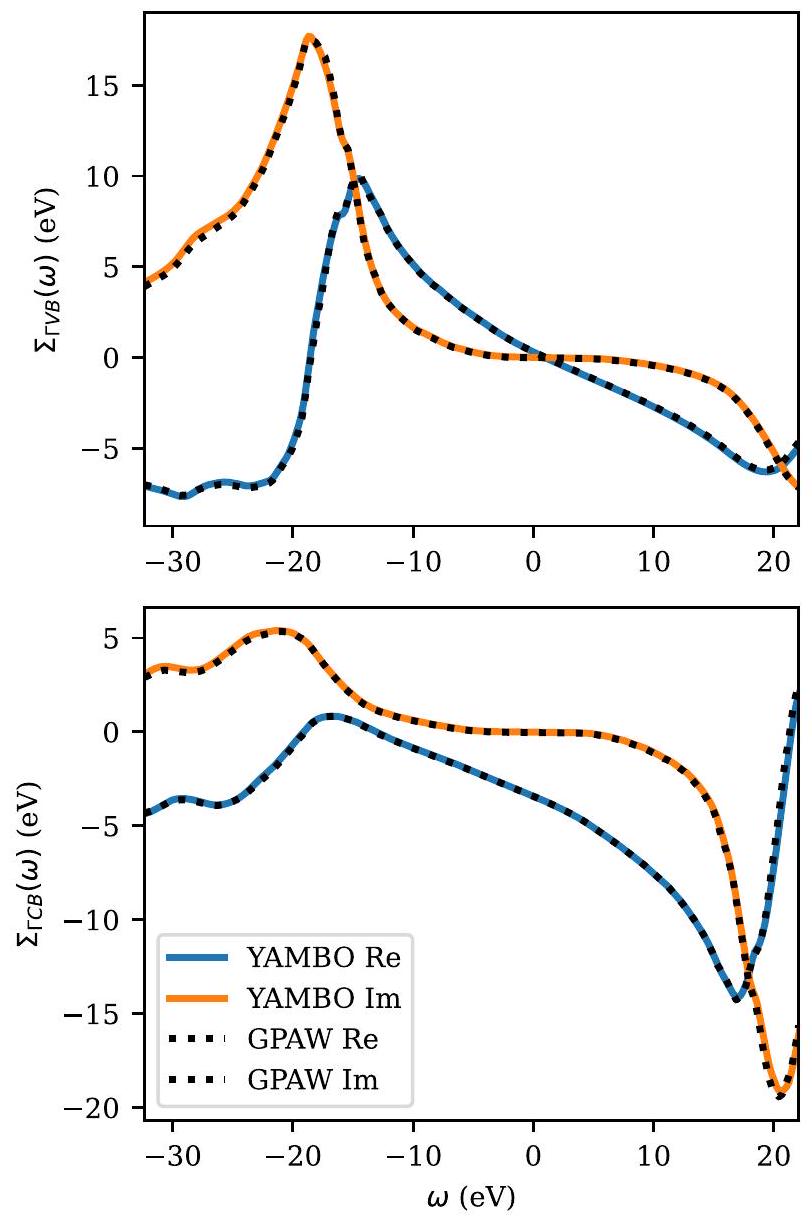
تظهر الشكل 9 عنصرين من المصفوفة للطاقة الذاتية الديناميكية GW لحالات نطاق التكافؤ ونطاق التوصيل عند نقطة غاما من السيليكون الكتلي. كما يمكن ملاحظته، فإن الاتفاق مع الكميات المقابلة التي تم الحصول عليها باستخدام كود Yambo GWمذهل.
معادلة بيته-سالبيتر (BSE)
بالإضافة إلى LR-TDDFT الم discussed في القسم VI A، يمكن تقريب دالة الاستجابة التفاعلية من خلال حل معادلة بيته-سالبيتر (BSE).على وجه الخصوص، بالنسبة لعدد موجي معينيمكن الحصول على الإثارات ذات الجسيمين من خلال تحويل هاملتونيان إلى الشكل القطري.
أينهي قيم eigen لـ Kohn-Sham وهي أرقام المهن المرتبطة. يتم تعريف النواة بواسطةمع
أينهو التفاعل الكهروستاتيكي الثابت المحدد في القسم VI E. يتم تقييم عناصر المصفوفة للنواة على أساس الموجة المستوية، حيث يمكن التعبير عنها بسهولة من حيث كثافات الأزواج (48) وتمثيل الفضاء العكسي لمصفوفة العزل (54).
في تقريب تام-دانكوف، يتم تجاهل اقتران الكتل الرنانة وغير الرنانة من هاملتوني BSE (تلك التي تتوافق مع طاقات الانتقال الإيجابية والسلبية، على التوالي). هذا يجعل هاملتوني BSE هيرميتي.يمكن كتابة دالة الاستجابة المتأخرة المتفاعلة على النحو التالي
الشكل 9. الأجزاء الحقيقية (Re) والتخييلية (lm) لعناصر مصفوفة الطاقة الذاتية عند نقطة غاما لشرائط التكافؤ (الأعلى) وشرائط التوصيل (الأسفل) تم تقييمها باستخدام Yambo وGPAW لسيليكون الكتلة. كلا الكودين يستخدمان تكامل ترددي كامل مع توسيع قدره 0.1 إلكترون فولت. يستخدم Yambo إمكانيات زائفة محافظة على النور، وGPAW هو إعداد PAW القياسي الخاص به. كانت شبكة نقاط kكان cutoff الموجة الطائرة 200 إلكترون فولت، وكان عدد النطاقات 200 لكلا الشيفرتين. النتائج تكاد تكون غير قابلة للتمييز.
أين
ويمثل القيمة الذاتية لمشغل هاملتونيان (73) المرتبطة بالمتجه الذاتي.
في GPAW، يتم بناء هاملتونيان BSE (73) على مرحلتين.أولاً، يتم حساب التفاعل المعزول الثابت عند جميع النقاط غير المتكافئة-نقاط في أساس الموجة المستوية، ثم يتم التعبير عن النواة بعد ذلك في أساس حالات KS ثنائية الجسيمات. الخطوة الأولى يتم توازيها بكفاءة على إما الحالات أو-نقاط، والخطوة الثانية موازية على كثافات الأزواج.
وبالتالي، يتم توزيع عناصر هاملتونيان على جميع وحدات المعالجة المركزية، ويتم إجراء التقطيع باستخدام ScaLAPACK بحيث لا يتم جمع الهاملتونيان الكامل على وحدة معالجة مركزية واحدة. لذلك، فإن أبعاد هاملتونيان BSE ومتطلبات الذاكرة محدودة فقط بعدد وحدات المعالجة المركزية المستخدمة في الحساب. نلاحظ أن التنفيذ ليس مقصورًا على تقريب تام-دانكوف، ولكن الحسابات تصبح أكثر تطلبًا بدونه. يمكن حساب دالة الاستجابة للأنظمة المتزاوجة في الدوران وكذلك الأنظمة المستقطبة في الدوران، ويمكن تضمين اقتران الدوران-المدار بشكل غير ذاتي.في الأنظمة ذات الأبعاد المنخفضة، من المهم القضاء على التغطية الزائفة من الصور الدورية للهيكل، وهو ما يتم تحقيقه من خلال تفاعل كولومب المقطوع في المرجع 208.
يمكن القول إن أهم تطبيق لـ BSE هو حساب طيف الامتصاص الضوئي للمواد الصلبة، حيث يوفر BSE حسابًا دقيقًا للتأثيرات المثيرة التي لا تلتقطها التقريبات شبه المحلية. (44). في الأنظمة ثنائية الأبعاد، تكون تأثيرات الإثارة ملحوظة بشكل خاص بسبب ضعف التغطية، وفي الشكل 10، نعرض القابلية القطبية ثنائية الأبعاد لـمحسوب من BSE مععند المقارنة مع الشكل 3، يُلاحظ أن حافة الامتصاص من المتوقع أن تكون موجودة عندنقطة، حيث يقوم اقتران الدوران-المدار بتقسيم أعلى نطاق تكافؤ بمقدار 0.45 إلكترون فولت. يُرى هذا التقسيم كقمتين مثيرتين تحت فجوة الطاقة، والتي تُفسر على أنها إثارة متميزة تنشأ من أعلى نطاق تكافؤ والنطاق التالي له (تقسيم أدنى نطاق توصيل غير ملحوظ في هذا الصدد). للمقارنة، نعرض أيضًا القابلية القطبية RPA، التي تم الحصول عليها باستخدام وحدة BSE من خلال تجاهل التفاعل المصفى في النواة، وهذا يظهر حافة الامتصاص المتوقعة عند فجوة الطاقة. وهذا يعطي نتائج متطابقة مع نهج معادلة دايسون في القسم VI A ولكنه يتمتع بميزة أن القيم الذاتية والأوزان في المعادلة (76) يتم الحصول عليها مباشرة، بحيث يتم تقليل التوسيع الاصطناعي.يمكن أن تتنوع دون تكلفة حسابية إضافية. كما أن تحليل الحالة الذاتية يتيح الوصول إلى “الحالات المظلمة”، ويكشف حساب BSE عن اثنين (واحد لكل وادٍ) من الإثارات الشبيهة بالثلاثيات التي تقع 70 ميغا إلكترون فولت تحت أدنى إثارة ساطعة في الشكل 10.
الشكل 10. القابلية القطبية ثنائية الأبعاد لـتم حسابه من BSE و RPA. في هذا الحساب، قمنا بتضمين اقتران الدوران-المدار واستخدمنا تقليم كولومب ثنائي الأبعاد لإزالة التغطية من الصور الدورية. شبكة نقاط k موحدة مركزة حول غاما منتم تطبيقه، وثماني حالات تكافؤ وثماني حالات توصيل (تم نقلها بمقدار 1 إلكترون فولت لمطابقة فجوة النطاق GW) ) تم تضمينها في تقريب تام-دانكوف. وهذا ينتج عنه هاملتونيان BSE بحجم معوالذي يمكن تحويله بسهولة إلى الشكل القطري باستخدام ScaLAPACK على 240 وحدة معالجة مركزية.
بالإضافة إلى الخصائص البصرية، يسمح GPAW بحل BSE عند النهايةوالتي يمكن استخدامها للحصول على علاقات انتشار البلاسمون من طيف فقدان طاقة الإلكترون (EELS) (57) وانتشارات الماجنون من القابلية المغناطيسية العرضية في القسم VI D.
ج. اقتران الإلكترون-الفونون
ترابط الإلكترون-الفونون هو مصدر لعدة خصائص مادية هامة، تتراوح من الموصلية الكهربائية والحرارية إلى الموصلية الفائقة. بالإضافة إلى ذلك، فإنه يوفر الوصول إلى إمكانيات التشوه، التي يمكن استخدامها للحصول على خصائص النقل للإلكترونات والثقوب في المواد الصلبة.
مصفوفة اقتران الإلكترون-الفونون من الدرجة الأولىيقيس قوة الربط بين فرع الفونونمع متجه الموجةوتكراروالحالات الإلكترونية و
مع
هنا، هو مجموع كتل جميع الذرات في وحدة الخلية، يدل على التدرج بالنسبة للإزاحات الذرية، و يُسقط التدرج في اتجاه إزاحات الفونونات. في حالة الأوضاع الثلاثة الانتقالية عندعنصر المصفوفةيختفي كنتيجة لقانون مجموع الصوت.
في GPAW،يتم تحديده باستخدام طريقة الفروق المحدودة مع وصف السوبرسيل للنظام. يمكن تنفيذ هذه الخطوة في أي من تمثيلات دالة الموجة المتاحة في GPAW. ثم يتم إسقاط المشتق على مجموعة من المدارات الذرية من قاعدة LCAO.، حيث تشير إلى فهرس الخلية و مؤشر المداري
تحويل فورييه من تمثيل بلوتش إلى تمثيل الفضاء الحقيقي يجعل من الممكن حسابلأي غرضأخيرًا، يتم الحصول على مصفوفة اقتران الإلكترون-الفونون من خلال إسقاط المصفوفة المقابلة للخلايا الفائقة إلى نطاقات وحدة الخلية الأولية.وأنماط الفونونات،
أينهي معاملات LCAO وهي متجهات إزاحة الفونونات على نطاق واسع.
طيف رامان
يصف تأثير رامان تشتت الضوء غير المرن، حيث يتم إثارة أوضاع الاهتزاز داخل المادة. يمكن حساب طيف رامان الرنيني وغير الرنيني للأنظمة المحدودة مثل الجزيئات في تقديرات مختلفة.يتم كتابة شدة رامان ستوكز بعد ذلك على أنها
أين يدل على وضع الفونون في بتردد و هو توزيع بوز-أينشتاين المقابل. علاوة على ذلك، و هي متجهات الاستقطاب للضوء الداخل والخارج، و تشير إلى موتر رامان لوضع الفونون .
النهج السائد لحساب يتضمن استخدام طريقة كرامرز-هايزنبرغ-ديراك (KHD). ضمن إطار KHD، يتم تحديد موتر رامان من خلال أخذ المشتق (باستخدام طريقة الفرق المحدود) للقطبية الكهربائية بالنسبة لوضعيات الاهتزاز الطبيعية. بدلاً من ذلك، يمكن للمرء استخدام نظرية الاضطراب من الدرجة الثالثة المعتمدة على الزمن لحساب موترات رامان. هذان النهجان متكافئان عندما تكون تأثيرات الحقل المحلي غير ملحوظة. ومع ذلك، يأتي كل نهج مع مجموعة من المزايا والعيوب الخاصة به. طريقة KHD أكثر كفاءة حسابية ولكنها محدودة في حساب عمليات رامان من الدرجة الأولى. يمكن توسيع نهج الاضطراب ليشمل عمليات رامان من درجات أعلى تتضمن عدة فونونات، لكنها تتطلب حسابات أكثر تطلبًا، مما يستلزم عددًا أكبر من النطاقات وشبكة k أكثر دقة لتحقيق التقارب. تم تنفيذ نهج الاضطراب في GPAW ويتم توضيحه أدناه، بينما تم تنفيذ طريقة KHD في حزمة ASR، باستخدام GPAW كخلفية حسابية.
في نهج الاضطراب، موتر رامان يُعطى بواسطة
حيث يُشار إلى الحد الأول على أنه الجزء الرنيني وتمثل الحدود المتبقية ترتيبات زمنية مختلفة للتفاعل من حيث مخططات فاينمان. هو عنصر مصفوفة الزخم بين النطاقات الإلكترونية و ، مع طاقة الانتقال في اتجاه الاستقطاب ، و هو قوة اقتران الإلكترون-فونون في الحد البصري كما هو معرف في المعادلة (82).
تظهر الشكل 11 طيف رامان المستقطب من bulk في المرحلة 2 H كما تم حسابه بتردد ليزر قدره . يستخدم هذا المثال الحد الرنيني فقط، حيث أن المساهمات الأخرى صغيرة في هذه الحالة. استخدمت هذه الحسابات قطع موجة مسطحة قدرها 700 eV وشبكة -نقطة في خلية فائقة . تم حساب ثوابت القوة والتغيرات المحتملة في نفس الوقت. يجب على المستخدمين التحقق بعناية من تقارب حجم الخلية الفائقة للفونونات والتغيرات المحتملة لكل نظام معين لتحقيق الدقة المطلوبة لمواقع الخطوط والشدة. نظرًا لأن حسابات طيف رامان تستخدم فقط فونونات ومصفوفات الإلكترون-فونون، فإن الخلايا الفائقة الصغيرة نسبيًا غالبًا ما تعطي نتائج مرضية.
الشكل 11. طيف رامان المستقطب من bulk في المرحلة 2 H عند . تم حساب الفونونات والتغيرات المحتملة باستخدام قطع موجة مسطحة قدرها 700 eV وشبكة -نقطة في خلية فائقة . تم تسمية كل قمة وفقًا لتمثيلها غير القابل للاختزال.
من الجدير بالذكر أننا أجرينا مقارنة بين الأطياف المحسوبة باستخدام حزمة ASR ولاحظنا مستوى عالٍ من الاتفاق لعدة مواد، على سبيل المثال، . تتماشى النتائج التي تم الحصول عليها من كلا الطريقتين عن كثب مع بعضها البعض من حيث مواقع القمم والقمم السائدة، ويمكن أن تُعزى الاختلافات الطفيفة بين الطريقتين إلى اختلافات في تفاصيل التنفيذ والاقترابات المميزة التي استخدمها كل منهما. على وجه التحديد، ضمن حزمة ASR، استخدمنا حزمة phonopy لحساب ترددات الفونون والموارد الذاتية، بينما في GPAW، قمنا مباشرة بحساب ترددات الفونون والموارد الذاتية باستخدام وحدة الفونون في ASE. علاوة على ذلك، في تنفيذ ASR، فرضنا بدقة تناظر موتر القطبية، وبالتالي، عادةً ما تظهر نتائج ASR التزامًا أكثر دقة بالتناظر المطلوب لموتر رامان مقارنةً بتنفيذ GPAW.
I. دوال الاستجابة البصرية التربيعية
يمكن الحصول على الاستجابة البصرية غير الخطية للمواد من خلال تجاوز نظرية الاضطراب من الدرجة الأولى. حاليًا، يقتصر تنفيذ GPAW على الاستجابة من الدرجة الثانية ضمن تقريب ثنائي القطب وبدون تضمين تأثيرات الحقل المحلي. نطبق تقريب الجسيم المستقل، الذي لا يمكنه التقاط السلوك الجماعي مثل تأثيرات الإثارة. يمكن كتابة حقل كهربائي متجانس مكانيًا في شكل مكوناته فورييه كما هو
حيث يمتد على الترددات الإيجابية والسلبية، تشير إلى المتجه الوحدوي على طول اتجاه -، و هو الحقل الكهربائي عند التردد . يمكن بعد ذلك التعبير عن كثافة الاستقطاب التربيعية المحفزة كما هو
حيث هو موتر الحساسية التربيعية من الرتبة 3. بسبب تناظر التبديل الداخلي، أي، ، يحتوي على 18 عنصرًا مستقلًا على الأكثر، والتي يمكن تقليلها أكثر بواسطة مبدأ نويمان وتناظر مجموعات النقاط. نلاحظ أن موتر التوصيل التربيعي المقابل يمكن اشتقاقه بسهولة من كـ بسبب العلاقة بين كثافة التيار وكثافة الاستقطاب.
من بين دوال الاستجابة المختلفة التي يمكن حسابها من ، قمنا بتنفيذ توليد التوافقيات الثانية (SHG) ومصفوفة التيار المتغير. يتطلب التنفيذ حاليًا تناظر عكس الزمن، مما يحد من التطبيق على الأنظمة غير المغناطيسية. بالنسبة لـ SHG، يتم فصل موتر الحساسية إلى حد نقي بين النطاقات وحد مختلط الذي يقرأ
هنا، ، حيث هو حجم البلورة، تشير إلى فرق السرعة بين النطاقات و ، و هو عنصر مصفوفة الموضع بين النطاقات ( )، الذي تم الحصول عليه من . تعتمد جميع الطاقات، والاحتلالات، وعناصر المصفوفة في التعبيرات السابقة على -المتجه. بالإضافة إلى ذلك، فإن الجمع على يعني تكاملًا على BZ الأول، أي، . تشير علامات الجمع المميزة إلى حذف الحدود ذات المؤشرات المتماثلة. أخيرًا، يتم تقييم المشتق العام (لـ ) باستخدام قاعدة الجمع
هنا، تم استبدال المجموعات اللانهائية بمجموعات محدودة، ولكن كبيرة، من النطاقات. من المهم التأكيد على أن كلا جانبي المعادلة يعتمد على -المتجه، وأن الجمع على الجانب الأيمن يتعلق فقط بالنطاقات. يجب أن يُذكر أن تنفيذًا آخر لموتر الحساسية التربيعية في مقياس السرعة متاح أيضًا في الكود
لكن لم يتم توثيقه هنا. بالنسبة لعدد كافٍ من النطاقات، تكون نتائج التنفيذين متطابقة.
فيما يتعلق بالتيار المتغير، حيث يتم تحفيز تيار مستمر استجابةً لحقل متناوب، يحتاج المرء إلى حساب موتر التوصيل التربيعي ,
في الممارسة العملية، يتم استبدال دالة دلتا بلورنتز مع اتساع محدود . لتجنب عدم الاستقرار العددي، يستخدم تنفيذ المعادلات (87)-(90) تسامحًا، بحيث يتم تجاهل الحدود إذا كانت الفروق الطاقية المرتبطة أو الفروق في مستويات فيرمي أصغر من التسامح. القيمة الافتراضية للتسامح هي و لفروق الطاقة ومستويات فيرمي، على التوالي.
VII. TDDFT في الوقت الحقيقي
تم تنفيذ مخطط TDDFT في الوقت الحقيقي (RT-TDDFT)، المعروف أيضًا باسم TDDFT للتطور الزمني، في ووضع LCAO . يتطلب شروط حدود غير دورية ولكنه غير مقيد بالنظام الخطي ويمكن تطبيقه لنمذجة الجزيئات في حقول قوية. يمكن دمج الطريقة مع النمذجة الكمية الكلاسيكية الهجينة لمحاكاة التفاعل الديناميكي بين الجزيئات ورنين البلازمون على أسطح المعادن. يعد LCAO-RT-TDDFT هو التنفيذ الأكثر حداثة، حيث يدعم تحليلات متعددة الاستخدامات ويمكّن من نمذجة أنظمة كبيرة بفضل كفاءته. نركز في هذا القسم على قدرات إصدار LCAO، ولكن بعض الوظائف الموصوفة متاحة أيضًا في وضع FD.
المعادلة الزمنية المعتمدة على KS في صيغة PAW هي
حيث يعتمد هاملتونيان كوهين-شام ضمنيًا على الزمن من خلال الكثافة المعتمدة على الزمن و هو جهد خارجي يعتمد على الزمن بشكل صريح. لقد افترضنا أيضًا أن مصفوفة التداخل مستقلة عن الزمن، أي أنه لا توجد ديناميات للأيونات.
بدءًا من الحالة الأساسية، يتم دفع المعادلة (91) عدديًا للأمام. بعد كل خطوة، يتم حساب كثافة جديدة، ويتم تحديثه وفقًا لذلك. يمكن للمستخدم تعريف الجهد الخارجي بحرية، وتشمل الجهود القياسية المنفذة دالة دلتا.ونبضة غاوسية، حيث هو مشغل ثنائي القطب في الاتجاه.
خلال الانتشار، يمكن تسجيل متغيرات زمنية مختلفة، وبعد الانتشار، يمكن معالجتها لاحقًا إلى كميات ذات اهتمام فيزيائي وكيميائي. كمثال أساسي، يمكن تحويل لحظة ثنائية القطب المعتمدة على الزمن المسجلة لاضطراب دلتا-كيك إلى طيف امتصاص الضوء باستخدام تحويل فورييه.يتم تسجيل الملاحظات من خلال ربط المراقبين بالحساب، وتشمل المراقبون المنفذين كتابًا لعزم ثنائي القطب، وعزم مغناطيسي، ومصفوفة كثافة KS في فضاء التردد، ودوال الموجة.
يمكن بدء حسابات RT-TDDFT من الحالة الأساسية أو الاستمرار من الحالة الأخيرة لانتشار زمني سابق، وتتيح ميزة محدد الوقت تحديد الوظائف إلى حد مسبق. كمية الوقت المستغرق. مع القدرة على الاستمرار، يسهل ذلك انتشار الوقت في قطع قصيرة، مما يتيح استخدام الموارد عالية الأداء المشتركة بكفاءة.
في تنفيذ LCAO-RT-TDDFT، يتم تحويل المعادلة (91) إلى معادلة مصفوفة وحلها باستخدام ScaLAPACK.تتم الخطوة الوسيطة لتحديث إمكانيات هارتري وXC على شبكة الفضاء الحقيقي.
أ. تحليل كوهين-شام
يمكن كتابة مصفوفة كثافة KS المعتمدة على الزمن كـ
أينهي المدارات الزمنية المعتمدة على كيه إس مع عوامل شغل الحالة الأساسيةمصفوفة كثافة KS هي كمية مركزية تتيح حساب الملاحظات ويمكن تقييمها بكفاءة في وضع LCAO.
تحويل فورييه لمصفوفة الكثافة المستحثةيمكن بناؤه في الوقت الحقيقي أثناء انتشار الزمن من خلال مراقب مصفوفة الكثافة. تم وصف التفاصيل المتعلقة بالتنفيذ في المرجع 54. مصفوفة كثافة KS في فضاء التردد مرتبطة بمتجهات eigen الخاصة بكاسيدا وتقدم معلومات مشابهة لحل معادلة كاسيدا.يمكن تحليل الكميات القابلة للرصد مثل الاستقطابية إلى مجموع على جزء الإلكترون-الثقب من مصفوفة كثافة كوهين-شام.، حيث . هذا يمكّن من إجراء تحليلات توضيحية، على سبيل المثال، من خلال التصوير المرئيعلى محاور الطاقة كخريطة لمساهمة الانتقال،التي يمكن من خلالها فهم طبيعة الرنين البلازمي السطحي المحلي (الشكل 12؛ انظر المرجع 54 لمناقشة مفصلة).
ب. تحليل الحاملات الساخنة
مصفوفة كثافة KS هي نقطة انطلاق عملية لتحليل توليد الحاملات الساخنة في الهياكل النانوية البلازمونية. في نطاق الاضطرابات الضعيفة، يمكن الحصول على مصفوفة كثافة KS الناتجة عن نبضات عشوائية من حسابات دالة دلتا.
الشكل 12. طيف امتصاص الضوء لـجزيئات نانوية على شكل إيكوساhedron وخريطة المساهمة الانتقالية عند 3.8 إلكترون فولت. تكشف الخريطة أن الانتقالات بين حالات KS القريبة من مستوى فيرمي تساهم بشكل بناء في رنين البلازما، بينما تساهم الانتقالات من الحالات المشغولة عند-حافة النطاق تساهم بشكل مدمر (التصفية).
روتين المعالجة اللاحقة.من خلال تحليل المصفوفة إلى مساهمات مكانية وطاقة مختلفة، يتم توليد حاملات ساخنة في الهياكل النانويةوعبر الجسيمات النانوية – أشباه الموصلاتوجزيئات النانويمكن دراسة الواجهات. تم توفير الأكواد الحاسوبية وسير العمل لمثل هذه التحليلات الخاصة بحاملات الحرارة في المراجع 245 و246.
ج. التشتت الدائري للجزيئات
التمييز الدائري الإلكتروني (ECD) هو طريقة طيفية قوية للتحقيق في الخصائص الكيرالية على المستوى الجزيئي. الكمية التي تميز ECD هي القوة الدورانية، التي تُعرف من خلال لحظة ثنائي القطب المغناطيسي.كما
حيث المؤشريعدد الاتجاهات الكارتيزية، الكتابة فوق السطر بين قوسين تشير إلى-اتجاه الركلة، وهو قوة الركلة. لحل، يحتاج المرء إلى أداء -دفع في جميع الاتجاهات الكارتيزية الثلاثة باستخدام حقل كهربائي مزعزعمكونات التردد لعزم ثنائي القطبيتم حسابها عن طريق تحويل فورييهالذي يتم تسجيله أثناء الانتشار. أخيرًا، يتم الحصول على لحظة ثنائي القطب المغناطيسي المعتمدة على الزمن كقيمة متوقعة للمشغل،
أينهو رقم الشغل لـمداري و هو حالة KS المتطورة زمنياً. يدعم تنفيذ GPAW الحالي كل من أوضاع FD و LCAO، وتتيح الكفاءة الحسابية لوضع LCAO حساب ECD للكتل النانوية المعدنية العضوية. يمكن العثور على مزيد من التفاصيل حول التنفيذ في المرجع 55.
د. إمكانات رد الفعل الإشعاعي
الاهتزازات الجزيئية البلازمونية أو الجماعية حساسة بشدة لأي نوع من التفاعل البصري. ستتزاوج التيارات المستحثة عبر معادلة الحركة لماكسويل مع البيئة البصرية وتؤدي إلى خسائر إشعاعية، أي، الانحدار نحو الحالة الأساسية. من الممكن حل مشكلة ماكسويل بشكل رسمي من خلال الحصول على موتر غرين.يمكن امتصاص التفاعل ثنائي القطب بين المجال الكهربائي والقطب الإلكتروني في جهد محلي.مناسب لـ Kohn-Sham TDDFT، حيث هو العزم الكهربائي الكلي. يمكن العثور على مناقشة مفصلة في المرجع 250.
بالنسبة للعديد من الهياكل البسيطة، مثل الفضاء الحر، والموجات أحادية البعد، أو الكرات العازلة،معروفة تحليليًا، ويمكن بعد ذلك تضمين الخسائر الإشعاعية في TDDFT دون تكلفة حسابية إضافية. الدروس التعليمية على صفحة GPAWتتضمن مثالاً على الموجات أحادية البعد حيث يمكن للمستخدم تحديد المساحة المقطعية واستقطاب الأوضاع المتنقلة. توسيع وظيفة جهد رد الفعل الإشعاعي إلى الفضاء الحر ثلاثي الأبعاد والتفاعل الجماعي لمجموعات كبيرة في تجاويف فابري-بروت من المبادئ الأساسية.ضروري لفهم كيمياء البولاريتون. هذه الوظيفة قيد التطوير حاليًا.
ديناميات إ. إهرنفست
تستند محاكاة الديناميكا الجزيئية (MD) عادةً إلى تقريب بورن-أوبنهايمر، حيث يُفترض أن النظام الإلكتروني يتفاعل بسرعة أكبر بكثير من النظام الأيوني، مما يجعله يصل إلى حالته الأساسية في كل خطوة زمنية. لذلك، يتم حساب القوى للديناميكا من كثافة الحالة الأساسية لنظرية الكثافة الوظيفية (DFT). بينما يكون هذا التقريب صالحًا بشكل كافٍ في معظم الحالات، هناك حالات يمكن أن تؤثر فيها الديناميكا الصريحة للنظام الإلكتروني على الديناميكا الجزيئية أو يمكن أن تؤثر فيها حركة الذرات على الخصائص الطيفية المتوسطة. يمكن التعامل مع هذه الحالات باستخدام ما يُعرف بديناميكا إرهينفست، أي الديناميكا الجزيئية لنظرية الكثافة الوظيفية المعتمدة على الزمن (TDDFT/MD).
تم تنفيذ ديناميات إهرنفست في وضع FD.يتوفر وصف للنظرية ودليل تعليمي على صفحة GPAW على الإنترنت.تم استخدام هذه الوظيفة لنمذجة التوقف الإلكتروني للأيونات بما في ذلك إثارة الإلكترونات الأساسية،دراسة نقل الشحنات عند الواجهات الهجينة في وجود الماء،محاكاة التشتت المتماسك لتيارات الذرات المحايدة من الجرافين،نموذج اعتماد كسر روابط الكربون تحتإشعاع الأيونات علىالهجينوكشف ديناميات نقل الشحنات عند أقطاب الكبريت المشحونة.تنفيذ LCAO، مستوحى من الأعمال الأخيرة في كود Siesta،قيد التطوير حاليًا.
ثامناً. طرق DFT للحالات المثارة
أ. المدارات الافتراضية المحسّنة
تقدم طريقة TDDFT للاستجابة الخطية عمومًا طاقات إثارة دقيقة بشكل معقول للحالات المثارة ذات القيمة المنخفضة، حيث تتداخل المدارات المرتبطة بالثقوب والإلكترونات المثارة بشكل كبير. ومع ذلك، فإنها تميل إلى الفشل في الإثارات التي تتضمن إعادة ترتيب مكاني للإلكترونات، مثل نقل الشحنة.رايدبرغوحالات مثارة مزدوجة.
يمكن تخفيف بعض هذه المشكلات من خلال استخدام الوظائف المفصولة حسب النطاق (انظر القسم III C 4). ومع ذلك، تأتي هذه الوظائف مع تكلفة حسابية مرتفعة بشكل كبير بسبب تقييم تكاملات التبادل. علاوة على ذلك، بسبب عدم وجود إلغاء لمصطلحات كولومب والتبادل للأوربيتال غير المشغولة الكانونية ضمن نظرية هارتري-فوك، يتم الحصول على أوربيتال غير مشغولة زائفة. وهذا يؤدي إلى تقارب بطيء لحسابات الاستجابة الخطية TDDFT بالنسبة لعدد الأوربيتال غير المشغولة عند استخدام الوظائف الهجينة والمفصولة حسب النطاق.
يمكن تحقيق تحسين كبير في التقارب فيما يتعلق بالأوربيتال غير المشغولة باستخدام أوربيتال افتراضية محسّنة، كما وضعها هوزيناجا وأرناو.في هذا النهج، يتم استخدام مشغل فوك المعدل للمدارات غير المشغولة، والذي يحاكي التفاعل بين ثقب مختار بشكل عشوائي من بين المدارات المشغولة في الحالة الأساسية والإلكترون المثار. يؤدي ذلك إلى تقارب أسرع في حسابات TDDFT ذات الاستجابة الخطية باستخدام الوظائف الهجينة والمفصولة عن المدى، كما أنه يجعل من الممكن تقييم خصائص الحالة المثارة. على سبيل المثال، يمكن الحصول على طاقة نقل الشحنة على المدى الطويل من خلال حسابات الحالة الأساسية لأن الفرق بين طاقة تقترب المدارات الافتراضية المحسّنة والثقب من طاقة الإثارة. تتوفر طريقة المدارات الافتراضية المحسّنة في GPAW، وتفاصيل التنفيذ موصوفة في المرجع 125.
ب. حسابات الحالة المثارة المتغيرة
يقدم GPAW أيضًا إمكانية إجراء حسابات الحالة المثارة باستخدام نهج بديل يعتمد على دالة الكثافة غير المعتمدة على الزمن. (يشار إليه أحيانًا بـ طريقة SCF)، التي لا تعاني من قيود الاستجابة الخطية TDDFT المذكورة في القسم الثامن A. تتضمن الطريقة تحسينًا تباينيًا للأوربيتال المرتبطة بحالة مثارة معينة من خلال تحسين الطاقة الإلكترونية إلى نقطة ثابتة غير الحالة الأساسية. الجهد الحسابي مشابه لذلك المستخدم في حسابات الحالة الأساسية، ويضمن التحسين التبايني أن يتم الوفاء بنظرية هيلمان-فاينمان. لذلك، يمكن استخدام جميع الآلات المتاحة في GPAW لتقييم القوى الذرية من أجل تحسين الهندسة ولتمثيل ديناميات الذرات في الحالة المثارة. علاوة على ذلك، فإن ربط هذه الطريقة التباينية المستقلة عن الزمن لحسابات الحالة المثارة مع إمكانيات MM الخارجية (انظر القسم الرابع) لا يتطلب جهود تنفيذ إضافية مقارنة بحسابات الحالة الأساسية ويوفر وسيلة لإجراء محاكاة ديناميات الجزيئات QM/MM في الحالة المثارة التي تشمل الاستجابة الخاصة بالحالة للمذيب، أي الاستجابة بسبب التغيرات في كثافة الإلكترون للذائب.
تتوافق الحالات المثارة المحسوبة بطريقة تباينية مع محددات سلاتر الفردية للأوربيتال المثلى مع شغل غير أوفباو، وعادة ما تكون نقاط سرج على سطح الطاقة الإلكترونية. وبالتالي، فإن الحسابات التباينية للحالات المثارة عرضة للانهيار إلى حلول ذات طاقة أقل، والتي تحافظ على تناظر التخمين الأولي. طريقة بسيطة للتداخل الأقصى (MOM)متاح في GPAW لمعالجة هذه المشكلة. في كل خطوة من خطوات SCF، يشغل MOM تلك المدارات التي تتداخل أكثر مع المدارات الخاصة بتخمين أولي غير أوفباو، والذي يتم الحصول عليه عادةً من حساب الحالة الأساسية. ومع ذلك، لا يضمن MOM تجنب الانهيار التغيري، وتكون مشاكل التقارب شائعة عند استخدام حلول eigen لـ SCF مع مخططات خلط الكثافة التي تم تطويرها لحسابات الحالة الأساسية.
1. تحسين المدارات المباشرة
لتخفيف المشكلات التي تؤدي إلى الانهيار التغيري وتحقيق تقارب أكثر موثوقية نحو حلول الحالة المثارة، يحتوي GPAW على استراتيجيتين بديلتين أكثر موثوقية من الحلول الذاتية التقليدية باستخدام MOM. تستند هذه الاستراتيجيات إلى تحسين مباشر للأوربيتالات وتستخدم خوارزميات بحث عن النقاط الحرجة مشابهة لتلك المستخدمة في بحث حالات الانتقال على أسطح الطاقة المحتملة لإعادة ترتيب الذرات. تسهل هذه الأساليب أيضًا حسابات الحالة المثارة التغيرية للوظائف غير الوحدوية، مثل الوظائف المصححة ذاتيًا (انظر القسم III C 5).
الطريقة الأولى من هذه الطرق هي نهج تحسين مداري مباشر مدعوم بطريقة MOM (DO-MOM). هذه الطريقة هي امتداد لنهج التخفيف المباشر باستخدام التحويل الأسي الموضح في القسم III B 5، حيث يكون البحث عن نقطة ثابتة عامة لـبدلاً من الحد الأدنى،
DO-MOM متاح في GPAW لكل من LCAO،شبكة الفضاء الحقيقي، ومجموعات الأساس للموجات المستوية.بالنسبة لقاعدة LCAO، فإن تحسين الحالة المثارة يتطلب فقط جعل الطاقة ثابتة بالنسبة لعناصر المصفوفة غير هيرميت. (زوايا دوران المدارات)، بينما تتضمن الحسابات باستخدام شبكة الفضاء الحقيقي والأساس الموجي المسطح تقليلًا في الحلقة الخارجية بالنسبة للمدارات المرجعيةتستخدم عملية التحسين في الفضاء الخطي للمصفوفات غير هيرميتية خوارزميات كوازية نيوتن فعالة يمكنها التعامل مع القيم الذاتية السلبية لمصفوفة هيسيان وبالتالي تتقارب نحو نقاط السرج. يقوم GPAW بتنفيذ خوارزمية جديدة ذات ذاكرة محدودة SR1 (L-SR1)، والتي أثبتت أنها قوية لحسابات الإثارات في الجزيئات.
يعتمد DO-MOM على تقدير درجات الحرية التي يجب أن يتم فيها تعظيم الطاقة، بدءًا من تخمين أولي. بالنسبة للإثارات التكافؤية وإثارات ريدبرغ، يتكون التخمين الأولي من مدارات الحالة الأساسية مع أعداد شغل غير بناءً على مبدأ أوفباو، مع تهيئة مسبقة باستخدام تقريب قطري لمصفوفة هيسيان الإلكترونية باستخدام طاقات المدارات.يمكن أن يكون كافياً. ومع ذلك، إذا كانت الإثارة تتضمن نقل شحنة كبير، يمكن أن تحدث إعادة ترتيب كبيرة في ترتيب طاقة المدارات، وقد يواجه DO-MOM صعوبة في التقارب. طريقة تحسين مباشرة ثانية مع متابعة الوضع العام (DO-GMF)يخفف هذه المشاكل ويتم تنفيذه أيضًا. في DO-GMF، مكونات تدرج الطاقةعلى طول الأنماطالموافق لـأدنى القيم الذاتية لمصفوفة هيسيان الإلكترونية معكوسة، مما يؤدي إلى
وتقليل باستخدام التدرج المعدليتم تنفيذها من خلال اتباعالأوضاع في وقت واحد. تضمن هذه العملية التقارب إلىنقطة السرج من الرتبة th، مما يلغي خطر الانهيار التغيري تمامًا. بينما هي أكثر تكلفة حسابيًا من DO-MOM بسبب الحاجة إلى تشخيص جزئي لمصفوفة هيسيان، فإن DO-GMF أكثر قوة. وبالتالي، فهي مفيدة بشكل خاص في استكشاف أسطح الطاقة المحتملة لأنها قادرة على متابعة حالة مثارة من خلال تكوينات كسر الروابط، حيث تظهر حلول كسر التماثل، من خلال استهداف الحل الذي يحافظ على ترتيب نقطة السرج. يتم تجسيد هذه الميزة المهمة من خلال التواء الرابطة المزدوجة الصعبة في الإيثيلين،حيث توفر حسابات DO-GMF للحالة المثارة المزدوجة الأدنى تقاطعًا متجنبًا مع الحالة الأساسية، في حين تفشل الطرق الأخرى في ذلك.
2. تطبيقات مثال على التحسين المباشر
تجعل كفاءة وموثوقية أساليب التحسين المباشر، جنبًا إلى جنب مع إمكانية اختيار أنواع مختلفة من مجموعات الأساس، الحسابات التغيرية للحالات المثارة في GPAW قابلة للتطبيق على مجموعة واسعة من الأنظمة تتراوح بين الجزيئات في الطور الغازي أو المحلول إلى المواد الصلبة.
يمكن أن يتيح الاسترخاء المداري المحدد للدولة وصف الإثارات الصعبة التي تتميز بإعادة ترتيب كثافة كبيرة. توضح الشكل 13 الخطأ في طاقة الإثارة العمودية لإثارة نقل الشحنة في جزيء N-phenylpyrrole الملتوي.تم الحصول عليها من خلال التحسين المباشر في GPAW باستخدام دالة LDA وPBE وBLYP وsz+aug-cc-pVDZأساس
الشكل 13. تطبيقات الحسابات المتغيرة غير الزمنية للحالات المثارة على جزيء في الفراغ (يسار)، جزيء في المحلول (وسط)، ونظام الحالة الصلبة (يمين). يسار: انحراف الطاقة المثارة المحسوبة لحالة مثارة من نوع نقل الشحنة في جزيء N-phenylpyrrole عن أفضل تقدير نظري لـ“نتائج حسابات TDDFT ذات الاستجابة الخطية باستخدام الوظائف الهجينة مأخوذة من المرجع 269. الوسط: تطور الزمن لزوايا الربط بين الجزيئات في [Cu(dmphen)معقد عند التحفيز الضوئي إلى أدنى حالة نقل الشحنة من المعدن إلى الليغاند (MLCT) في الأسيتونيتريل. النتائج التجريبية من قياسات تشتت الأشعة السينية بالفيمتوثانيةيتم مقارنتها بالمتوسط عبر مسارات الديناميكا الجزيئية في الحالة المثارة التي تم الحصول عليها باستخدام نظام تضمين الكهروستاتيكي QM/MM في GPAW (انظر القسم الرابع) ومتشابك مع دالة استجابة الجهاز التجريبي.اليمين: طاقة الإثارة العمودية للإثارات في مركز النيتروجين-الفراغ المشحون سلبًا في الماس التي تم الحصول عليها باستخداموظيفة SCAN مقارنةً بنتائج الحسابات السابقة باستخدام نهج تضمين كمي متقدم.تُعرض المدارات المشاركة في الانتقالات الإلكترونية في الصورة المرفقة (ذرات الكربون باللون الرمادي وذرة النيتروجين باللون البرتقالي).
تم تعيينه مقارنةً بنتائج حسابات TDDFT ذات الاستجابة الخطية بنفس مجموعة الأساس والدوال، بالإضافة إلى الدوال الهجينة PBE0 و B3LYP (نتائج من المرجع 269). بالنسبة للحسابات التباينية، يتم حساب طاقة الحالة المثارة المفردة باستخدام صيغة تنقية الدوران.، حيث هي طاقة حالة مختلطة للدوران تم الحصول عليها من خلال ترقية إلكترون في قناة دوران واحدة وهو طاقة الحالة الثلاثية بنفس الخصائص. تقديرات التباين تقلل من القيمة النظرية الأفضل لتقدير طاقة الإثارة (5.58 إلكترون فولت) في المرجع 269 بمقدارخطأ أصغر بكثير من ذلك الناتج عن حسابات TDDFT ذات الاستجابة الخطية باستخدام نفس الوظائف ( -2.0 eV ) أو مع الوظيفة الهجينة PBE0 الأكثر استهلاكًا للحسابات ( -0.85 eV ).
تم استخدام الطريقة أيضًا لمحاكاة التغيرات الهيكلية الناتجة عن الضوء في المعقدات المعدنية المحفزة للضوء والديناميات المائية المصاحبة.تظهر الشكل 13 تطبيقًا لمستشعر الضوء النموذجي لمركب النحاس.(dmphen = 2,9-dيميثيل-1,10-فينانثرولين) في الأسيتونيتريل، حيث أوضحت محاكاة الديناميكا الجزيئية QM/MM تفاعلًا معقدًا بين تشوه الروابط وإعادة ترتيب جزيئات المذيب المحيطة بعد إثارة ضوئية إلى حالة نقل الشحنة من المعدن إلى الرابط.
المثال الأخير للتطبيق المعروض في الشكل 13 هو حساب الحالات المثارة لنظام الحالة الصلبة،مركز النيتروجين-الفراغ المشحون سلبًا في الماس، والذي يتكون من عيب نموذجي للتطبيقات الكمية. يتم وصف النظام باستخدام سوبرسيل كبير مكون من 511 ذرة، وتستخدم الحسابات مجموعة أساس من الموجات المستوية. على عكس التقارير السابقة، تم العثور على مجموعة من الوظائف الكثافة المختلفة التي تعطي الطاقة الصحيحة. ترتيب الحالات المثارة، معوظيفة SCAN توفر أفضل توافق مع حسابات التضمين الكمي ذات الجسم المتعدد على مستوى عالٍ مع خطأ أقل منهذا المثال يظهر أن طرق التحسين المباشر في GPAW هي أدوات واعدة لمحاكاة الحالات المثارة في الأنظمة الممتدة، حيث تكون الطرق البديلة إما مكلفة حسابياً أو تفتقر إلى الدقة.
IX. ميزات أخرى
أ. الاستقطاب الكهربائي
يمكن حساب الاستقطاب الرسمي للمواد السائبة من النظرية الحديثة للاستقطاب.كما
أين
هل المساهمة الإلكترونية و
هو المساهمة من النوى. هنا، تتجمع المجموعات على الذرات في الخلية الوحدة وهو شحنة النواة (بما في ذلك الإلكترونات الأساسية)، الواقعة في الموقع يمكن اعتبار المساهمة الإلكترونية كتكامل منطقة بريلوان لـ-مساحات بيري الفضائية ويمكن تقييمها من نسخة الفرق المحدود من المعادلة (98).
يتعلق هذا بالتداخلات بين المدارات بلوخ عند نقاط k المجاورة، والتي من السهل تقييمها في صيغة PAW.
المعادلة (97) معرفة فقط بالمودول، الذي يتبع من الاختيار التعسفي لوحدة الخلية لمواقع الذرات بالإضافة إلى اختيار الأطوار لـالذي يمكن أن يغير طور بيري بواسطةومع ذلك، فإن التغير في الاستقطاب تحت أي تشوه أديباتيكي محدد جيدًا ويمكن حسابه على النحو التالي
أينهو متغير بلا أبعاد يحدد المسار الأديباتي. بشكل خاص، بالنسبة للمواد الفيروكهربائية، فإن الاستقطاب التلقائييمكن تقييمه من خلال اختيار مسار يشوه الهيكل من الحالة القطبية الأساسية عندإلى هيكل غير قطبي في.
في الشكل 14، نعرض مثالاً على ذلك للهيكل الرباعي.وهو معروف بأنه مادة كهرضغطية.تم تخفيف الهيكل القطبي تحت قيد التناظر الرباعي باستخدام PBEثم تم الاستيفاء الخطي إلى الهيكل المعكوس (يمر عبر نقطة مركزية التماثل عندهناك عدد لا نهائي من فروع الاستقطاب تختلف حسب كم الاستقطاب ( كونه ثابت الشبكة في-الاتجاه)، ويتم الحصول على الاستقطاب العفوي من خلال اختيار فرع واحد وتقييم الفرق في الاستقطاب الرسمي عند و من المثير للاهتمام أن النقطة المركزية لها استقطاب غير معدوم يعطى بنصف كمية الاستقطاب. هذا مسموح به بسبب الطبيعة متعددة القيم للاستقطاب الرسمي، وقد أظهرت مثل هذه “الاستقطاب الطوبولوجي” في المواد غير القطبية أنها تؤدي إلى حالات سطحية بلا فجوة.هنا، ومع ذلك، نستخدم فقط الاستقطاب الطوبولوجي لتأكيد أهمية تقييم الاستقطاب العفوي كالتغيير فيعلى طول مسار عازل حرارياً.
الشكل 14. الاستقطاب الرسمي على طول مسار أديوباتي يربط بين حالتين من الاستقطاب والطاقة على طول المسار في الشكل الرباعي.يتم الحصول على الاستقطاب العفوي كفرق في الاستقطاب بين حالة أرضية قطبية ) وهي بنية مرجعية غير قطبية ( ). يتم أيضًا عرض الطاقة على طول المسار.
يمكن تطبيق التعبيرات (97)-(100) لاستخراج خصائص مختلفة للمواد غير القطبية أيضًا، على سبيل المثال، موترات الشحنة الفعالة لبورن.
التي تعطي التغير في الاستقطاب الناتج عن التحولات الصغيرة في مواقع الذرات. في GPAW، يتم الحصول على هذه من خلال استدعاء بسيط لوحدة تقوم بإدخال (تحول محدد من قبل المستخدم) لجميع الذرات في الخلية الوحدة وتحسب التغير الناتج في الاستقطاب من المعادلات (97)-(99). يمكن دمج شحنات بورن مع مصفوفة القوة الذرية لحساب المواقع التوازنية تحت تأثير مجال كهربائي ثابت، ويمكن حساب مساهمة الشبكة في الاستقطاب الديناميكي من القيم الذاتية والمتجهات الذاتية لمصفوفة القوة.بالإضافة إلى ذلك، يمكن الحصول على الاستجابة الكهروضغطية من خلال حساب التغير في الاستقطاب استجابةً للإجهاد الخارجي.مساهمة الشبكة في الاستقطابية عادة ما تكون أقل بكثير من الجزء الإلكتروني، ولكن بالنسبة للمواد الفيروكهربائية، يمكن أن تؤدي أوضاع الفونونات اللينة المرتبطة بالاستقطاب التلقائي إلى استقطابيات شبكية كبيرة.
نحن نوضح ذلك في الحالة المعروفة للمواد الفيروكهربائية ثنائية الأبعاد GeS،حيث نحصل على استقطاب عفوي قدره 490في توافق ممتاز مع الحسابات السابقة.الخصائص القطبية في المستوى ثنائي الأبعاد للشبكة والإلكترونيات هي و على التوالي.للمقارنة، فإن الحالة غير القطبية لـ 2D MoS2 تعطي و
ب. مراحل بيري وطوبولوجيا النطاق
تعتمد الأطوار الطوبولوجية مثل حالة هول الكم وموصل تشيرن بشكل حاسم على وجود اقتران الدوران-المدار، ويمكن الحصول على طوبولوجيا النطاق من تطور-مساحات بيري عبر منطقة بريلوان. بشكل خاص، بالنسبة للعوازل، القيم الذاتية لمصفوفة طور بيري للحالات المشغولة
يجب أن يتغير بمضاعف صحيح منعندما يكون مكون من (مكونات عمودي على ) يتم تدويره عبر منطقة بريلوان.هناهي حالات بلوتش السبينور، والتي عادةً ما تكون ليست دوالًا سلسة لـلذا فإن تقييم المعادلة (102) يتطلب بناء مقياس سلس، وفي GPAW، يتم التعامل مع ذلك بواسطة خوارزمية النقل المتوازي من المرجع 286.
تم تطبيق الطريقة على بحث عالي الإنتاجية عن مواد ثنائية الأبعاد طوبولوجية جديدة،وفي الشكل 15، نعرض مراحل بيري المحسوبة لـنظرًا لتماثل عكس الزمن، فإن مراحل بيري عند و تكون مزدوجة من حيث الطاقات، وبالتالي لا يمكن لأي اضطراب يحافظ على تناظر عكس الزمن أن يفتح فجوة في طيف مرحلة بيري. هذه الخاصية تشخص حالة العزل الكمي للدوران وهي مرتبطة ارتباطًا وثيقًا بوجود حالات حافة بلا فجوة.
يمكن أيضًا استخدام القيم الذاتية للمعادلة (102) لحساب المساهمة الإلكترونية في الاستقطاب الرسمي، حيث إن مجموع جميع مراحل بيري الفردية يعطي نفس القيمة التي يمكن الحصول عليها من المعادلة (98). ومع ذلك، فإن النهج الحالي أكثر تعقيدًا لأنه يتطلب بناء مقياس سلس، وهو ما لا يحتاجه في المعادلة (98).
الشكل 15. مراحل التوت من العازل الكمي للدورانالمستمدة من PBE مع اقتران الدوران غير الذاتي. الألوان تشير إلى قيمة التوقع لـلكل حالة كما هو محدد في المرجع 46.
C. دوال وانير
توفر دوال وانير (WFs) تمثيلاً محليًا للحالات الإلكترونية لمادة صلبة. يتم تعريف دوال WFs من خلال تحويل موحد للحالات الذاتية لبلاخ الذي يقلل من الامتداد المكاني للأوربيتال الناتج. بشكل محدد،دالة وانير رقمفي وحدة الخلية
تكتب كـحيثهي دالة بلاخ عامة (تراكب للحالات الذاتية لبلاخ عند
).إن تقليل الامتداد المكاني لمجموعة من دوال WFs
يعادل زيادة الوظيفة الموزعة
حيثالمجموعةهي مجموعة من ستة متجهات معكوسة على الأكثر تربط نقطةإلى جيرانها، و
هي الأوزان المقابلة التي تأخذ في الاعتبار شكل وحدة الخلية.تحدد دوال بلاخ العامة في المعادلة (103) من خلال تقليل
باستخدام، على سبيل المثال، مخطط التدرج المترافق كما هو مطبق في وحدة وانير ASE. المدخلات إلى خوارزمية وانير هذه هي المصفوفاتحيث هي تصحيحات PAW من المعادلة (8). من هذه المصفوفات، يمكن استخدام وحدة وانير ASE لبناء دوال وانير مشغولة جزئيًا،وهي تعميم لدوال وانير المحلية بشكل أقصىللنطاقات المتشابكة والأنظمة غير الدورية. مؤخرًا، تم تحقيق تحسين إضافي من حيث متانة إجراء وانير باستخدام وظيفة موزعة معدلة تحتوي على مصطلح عقوبة يتناسب مع تباين توزيع الانتشار لدوال WFs، مما يؤدي إلى توزيع أكثر تجانسًا.
D. حسابات العيوب النقطية باستخدام الوظائف الهجينة
تلعب العيوب النقطية دورًا حاسمًا في العديد من تطبيقات أشباه الموصلات.يمكن استخدام حسابات المبادئ الأولى لتحديد الهيكل الذري، طاقة التكوين، ومستويات انتقال الشحنة للعيوب النقطية. من المعروف جيدًا أن أفضل وصف للعيوب النقطية في أشباه الموصلات/العوازل يتم الحصول عليه باستخدام هجينة مفصولة النطاق، مثل الوظيفة الهجينة HSE06.لتوضيح استخدام GPAW لحسابات العيوب النقطية، نحدد مخططات طاقة التكوين للعيوبوفي بلورة نيتريد البورون السداسي (hBN) باستخدام الوظيفة HSE06. تم اقتراح أن هذه العيوب مسؤولة عن إشارة اللمعان ذات المستوى العميق مع خط فوني صفر (ZPL) حولتتم مقارنة النتائج مع نتائج مماثلة تم الحصول عليها باستخدام حزمة البرمجيات VASP.بالنسبة لعيب نقطي D في حالة الشحنة
يتم حساب طاقة التكوينمن المعادلة،هنا،
وهي الطاقات الكلية للبلورة مع العيب النقطي في حالة الشحنةوللبلورة النقية المحايدة، على التوالي.هو الجهد الكيميائي للعنصربينماهو عدد الذرات المضافة إلى () أو المزالة من () البلورة لإنشاء العيب.هو الجهد الكيميائي للإلكترونات، أي مستوى فيرمي، الذي يكتب كـحيث VBM هو الحد الأقصى لحزمة التكافؤ. أخيرًا،هو مصطلح تصحيح يأخذ في الاعتبار (i) التفاعل الكهروستاتيكي الزائف بين الصور الدورية للعيب وتفاعلها مع الشحنة الخلفية المتجانسة التعويضية و(ii) التحول المحتمل بين الأنظمة النقية والعيوب.للحصول على مزيد من التفاصيل حول منهجية حسابات العيوب النقطية، نوجه القارئ إلى الأوراق الاستعراضية الممتازة حول هذا الموضوع.
تم إجراء جميع الحسابات باستخدام الوظيفة HSE06 مع معامل الخلط الافتراضي
وقطع موجة مستوية قدره 800 eV، والقوى المتقاربة إلىÅÅÅ-نقاط)، بما يتماشى جيدًا مع فجوة الطاقة التجريبية لـتم استرخاء هيكل العيوب النقطية في(128 ذرة) باستخدامنقطة-نقطة أخذ العينات. بالنسبة لكل عيب، تم اعتبار ثلاث حالات شحنة مختلفة () تم تقييم التصحيحات () بسبب شحنات الصورة ومحاذاة الجهد وفقًا لـ Freysoldt وNeugebauer وVan de Walleكما هو مطبق في GPAW.تظهر الشكل 16 طاقات تكوين العيوب كدالة لمستوى فيرمي لـ
وفي ظروف غنية بالنيتروجين وفقيرة بالنيتروجين، على التوالي. يمكننا أن نرى أنه تحت ظروف غنية بالنيتروجين،هو طاقةالشكل 16. طاقات تكوين العيوب لـ
وتحت ظروف غنية بالنيتروجين وفقيرة بالنيتروجين، على التوالي. الخطوط المتقطعة مستنسخة من المرجع 295.أقل، بينما
مفضل تحت ظروف فقيرة بالنيتروجين.يظهر انتقال شحنة 1/0 عند 3.73 eV فوق VBM، بينمالديه انتقال شحنةعند 3.26 eV داخل فجوة الطاقة. نجد توافقًا جيدًا مع دراسة مماثلةتستخدم أيضًا الموجات المستوية والوظيفة HSE06 (حسابات VASP). يمكن أن تُعزى التباينات الطفيفة إلى استخدام حجم خلية سوبر مختلفة ونسبة أعلى قليلاً من معامل الخلط غير المحلي ().
E. تمثيلات تناظر مجموعة النقاط
يسمح GPAW بالتعيين الآلي لتمثيلات تناظر مجموعة النقاط لدوال كوهين-شام المحسوبة مسبقًا. يمكن استخدام ذلك لتحديد تمثيلات تناظر دالة الموجة لكل من الجزيئات
والهياكل الممتدةلتحليل، على سبيل المثال، التناظر المتضمن في تدهور النطاقات وقواعد الاختيار للانتقالات ثنائية القطب.يتبع التحليل مباشرة من نظرية المجموعات،
التي تنص على أن الحلول لمعادلة شرودنجر ترث مجموعة التناظر للهميلتوني المعني، أو أساسًا الجهد الخارجي المستدعى بواسطة التكوين الذري. يتم حساب مصفوفات التمثيلكـحيث
هي دالة موجة طبيعية،هي تسمية الحالة الذاتية، وهي عملية تتوافق مع التحويللمجموعة التناظر للهميلتوني. تشمل العملياتالتدويرات التي تكون غير تافهة للشبكة المستطيلة التي يتم إسقاط دوال الموجة المحسوبة عليها. يتم إجراء تدويرات دالة الموجة على الشبكة بواسطة الاستيفاء التكعيبي. تحتوي مخرجات التحليل على أوزان التمثيل غير القابل للاختزاللكل حالة ذاتيةكما تم حلها منحيث
هي متجهات الشخصية للمجموعة (أي، صفوف جدول الشخصية).عند إجراء التحليل، يحتاج المستخدم إلى إدخال إحداثيات مركز التناظر (عادةً إحداثيات ذرة واحدة) ومجموعة النقاط التي يتم تشغيل التحليل من أجلها. من الممكن تحليل جزء فقط من دالة الموجة عن طريق اختيار نصف قطر قطع من مركز التناظر يتجاوزها أجزاء من
دالة الموجة يتم تجاهلها. يتيح ذلك التحقيق في نقاء التناظر المحلي حتى لو كان تناظر الهميلتوني مكسورًا بعيدًا عن مركز التناظر. حتى الآن، تم تنفيذ مجموعات النقاط منوو.
F. تفكيك هيكل النطاق
عند دراسة تكوين العيوب، أو مراحل مرتبة للشحنة، أو انتقالات هيكلية، غالبًا ما يكون من الضروري إجراء حسابات DFT على خلية سوبر. تأتي حسابات الخلية السوبر (SC) مع تكلفة الحاجة إلى حساب المزيد من الإلكترونات في وحدة الخلية مقارنةً بالخلية الأولية (PC). وهذا يعني أنه، بالإضافة إلى زيادة الجهد الحاسوبي، يحتوي هيكل النطاق لخلية SC على المزيد من النطاقات في منطقة بريلوان أصغر مقارنةً بـ PC. من أجل مقارنة الهياكل الإلكترونية للنطاقات بين SC وPC، يصبح تفكيك هيكل النطاق لخلية SC إلى هيكل الخلية الأولية (PC) مريحًا.
يتميز GPAW بإمكانية إجراء تفكيك هيكل النطاق في شبكة الفضاء الحقيقي، والموجة المستوية، وأنماط LCAO. يسمح التنفيذ بتفكيك هيكل النطاق لخلية SC دون الحساب الصريح للتداخل بين دوال الموجة SC وPC، وفقًا للإجراء الموصوف في المرجع 307. يتم إعطاء هيكل النطاق المفكك من حيث الوظيفة الطيفية
معوالزخم في مناطق بريلوان PC وSC، على التوالي (مرتبط بشكل فريد بـبواسطة متجهمن SC).هي القيم الذاتية لـ SC التي تم الحصول عليها للزخمومؤشر النطاقويتم حسابه كـ
حيثهي معاملات فورييه للحالة الذاتيةو هو مجموعة من متجهات الفضاء العكسي لـ SC التي تتطابق مع متجهات الفضاء العكسي لـ PC. يمكن العثور على شرح أكثر تفصيلاً وتفاصيل تقنية حول كيفية إجراء تفكيك هيكل النطاق على صفحة GPAW.
G. نموذج QEH
الهيكل غير المتجانس الكمي-الكهربائي (QEH النموذج هو ميزة إضافية في GPAW لحساب الاستجابة العازلة والإثارات في أكوام عمودية من المواد ثنائية الأبعاد، والمعروفة أيضًا باسم الهياكل غير المتجانسة (vdW). يمكن استخدام نموذج QEH بشكل مستقل عن كود GPAW، لكنه يعتمد على تنفيذ GPAW لحساب الكتل الأساسية المستخدمة في النموذج، كما هو موضح أدناه.
تكون الشاشة العازلة في المواد ثنائية الأبعاد حساسة بشكل خاص للتغيرات في البيئة وتعتمد على ترتيب التكديس وسمك الهيكل غير المتجانس ثنائي الأبعاد، مما يوفر وسيلة لضبط الإثارات الإلكترونية، بما في ذلك فجوات النطاق شبه الجسيمات والإثارات. بينما يمكن تمثيل الاستجابة العازلة للطبقات المستقلة بشكل صريح من البداية في GPAW على مستويات نظرية الاستجابة الخطية TDDFT وGW وBSE، فإن عدم تطابق الشبكة بين طبقات ثنائية الأبعاد المختلفة غالبًا ما يؤدي إلى خلايا فائقة كبيرة تجعل هذه الأساليب متعددة الجسيمات غير قابلة للتطبيق. نظرًا لأن التفاعل بين
الطبقات المكدسة يتم التحكم فيه عمومًا بواسطة تفاعلات فان دير فالس، فإن التعديل الرئيسي على استجابة الطبقات غير المتفاعلة ينشأ من الاقتران الكهربائي طويل المدى بين الطبقات.
لذلك، في نموذج QEH، يتم الحصول على الدالة العازلة للهيكل غير المتجانس vdW من خلال اقتران كهربائي لكتل العازلة الكمية للطبقات ثنائية الأبعاد الفردية. تتكون كتل العازلة من مكونات أحادية القطب وثنائية القطب لدالة الاستجابة الكثافية للطبقات المستقلة،، المحسوبة من من البداية على مستوى RPA. بعد ذلك، يتم حساب دالة الاستجابة الكثافية الكاملة (اضطراب الكثافة على الطبقة بسبب مكون أحادي القطب أو ثنائي القطب للحقل المثير الذي يؤثر على الطبقة ) عن طريق حل معادلة دايسون
حيث يتم الحصول على عنصر مصفوفة كولوم من التداخل في الفضاء الحقيقي على الكثافة،، والجهد،، دوال الأساس على الطبقات المختلفة،
من دالة الاستجابة الكثافية، يتم الحصول على الدالة العازلة على أساس اضطرابات أحادية القطب/ثنائية القطب على كل طبقة في الهيكل غير المتجانس. بينما يتم توفير كتل البناء المحسوبة مسبقًا باستخدام GPAW لمجموعة كبيرة من المواد ثنائية الأبعاد مع حزمة QEH، تقدم GPAW إمكانية حساب كتل بناء مخصصة لأي مادة ثنائية الأبعاد، كما هو موضح في المرجع 310.
كمثال توضيحي لنموذج QEH، نوضح كيف يمكن هندسة الدالة العازلة الثابتة لهيكل غير متجانس من خلال التكديس متعدد الطبقات. توضح الشكل 17 الدالة العازلة الثابتة لهيكل غير متجانس vdW يتكون من طبقات و
الشكل 17. الدالة العازلة الماكروسكوبية الثابتة لواجهة الهيكل غير المتجانس vdW كدالة لعدد الطبقات. يتكون الهيكل غير المتجانس من طبقات في نصف واحد و طبقات في النصف الآخر (انظر الشكل المصغر). يؤدي زيادة عدد الطبقات في النهاية إلى حد يشبه الكتلة لتكوين التكديس المختار.
طبقات. نرى أن الدالة العازلة تزداد بشكل كبير كدالة لعدد الطبقات، مما يقترب في النهاية من حد الكتلة. يمكن استغلال معرفة اعتماد الاستجابة العازلة على الطبقة لمثل هذا الهيكل غير المتجانس بشكل أكبر للتحقيق في خصائص الإثارة بين الطبقات وداخلها وتأثيرات إعادة تشكيل حافة النطاق.
H. نماذج المذيبات
لوجود مذيب تأثير كبير على الديناميات والبنية الإلكترونية للجزيئات أو الأسطح الممتدة. على وجه الخصوص، فإن المذيب الأكثر أهمية، الماء، قادر على استقرار الأيونات، أو الأيونات الثنائية، التي لن تتشكل في الطور الغازي. يتعلق التأثير الرئيسي بالسمية الكبيرة للماء () التي تعزل بشكل فعال تفاعلات كولوم.
طريقة مريحة وقليلة الحسابات لوصف هذا التأثير هي تضمين سُمك المذيب المعتمد على الموضع في الكهروستاتيكا عبر حل بواسون. يتم تمثيل المذيب فقط كاستمرارية قابلة للاستقطاب تقوم بمتوسط جميع الحركات وإعادة ترتيب جزيئات المذيب وإلكتروناتها. لذلك، فإن التكلفة الحسابية هي، عمليًا، نفس تكلفة الحساب في الفراغ.
تسمح هذه التنفيذ بحساب طاقات الذوبان الحرة للأنواع المحايدة والأيونية في المحلول. يتم وصف طبيعة المذيب بواسطة سُمكه، وهو جهد طرد فعال يميز توزيع المذيب السلس حول المذاب، وتوتر سطحي فعال يلخص التفاعلات المشتتة والطاردة بين المذاب والمذيب. لذلك، فإن الوصف مناسب تمامًا لأي مذيب يمكن تمثيله بشكل فعال بواسطة استمرارية، حيث عادةً ما تظهر المذيبات ذات السمية العالية أكبر التأثيرات. يمكن اعتبار التفاعلات المحلية بين المذاب والمذيب مثل الروابط الهيدروجينية من خلال التضمين الصريح لجزيئات مذيب فردية كجزء من المذاب. يعمل نموذج المذيب مع ظروف حدود دورية وكذلك محدودة ولكن متاح حتى الآن لوحدات LCAO وFD فقط. يمكن تطبيق النموذج بشكل أكبر على الأسطح الدورية المتصلة مع إلكتروليت لإعادة إنتاج انخفاضات محتملة معقولة ضمن محاكاة عمليات التفاعل الكهروكيميائية، كما سنوضح في ما يلي.
I. واجهات كهروكيميائية مشحونة
إن محاكاة العمليات الذرية عند واجهة صلبة-سائلة تحت جهد إلكترودي محكوم يتم بشكل أكثر ملاءمة في التجميع الإلكتروني الكبير. هنا، يمكن تبادل الإلكترونات ديناميكيًا مع خزان إلكتروني خارجي عند جهد كهروكيميائي محدد جيدًا. في نظام دوري، سيؤدي الشحن الصافي غير الصفري إلى تباين الطاقة؛ لذلك، يجب تعويض أي إلكترونات جزئية تتم إضافتها إلى النظام أو إزالتها بمقدار متساوي من الشحنة المعاكسة. تم تقديم عدة طرق قادرة على حساب هذا التغيير في ظروف الحدود مؤخرًا. في GPAW، يتم تحقيق ذلك بشكل مريح من خلال إدخال شريحة جليوم من شحنة متساوية ومعاكسة للشحنة الإلكترونية المطلوبة؛ يتم تضمين الجليوم في مذيب ضمني محلي في منطقة الفراغ فوق السطح المحاكى (انظر القسم IX H). كميزة خاصة من هذه الطريقة المعروفة باسم طريقة الجليوم المذاب (SJM)، كما هو معروف في GPAW، نحن قادرون على تحديد الشحنة الزائدة على الجانب العلوي فقط من السطح الذري المحاكى، والذي يحدث بشكل طبيعي من خلال
إدخال منطقة الجليوم فقط في الفراغ العلوي وفصل الجانبين من الخلية كهربائيًا عبر تصحيح ثنائي القطب. يمكن تطبيق كل من مذيب ضمني بحت ومذيب هجين صريح-ضمني.
في SJM، يكون الجهد الإلكتروني المحاكى دالة أحادية من عدد الإلكترونات في المحاكاة؛ يمكن إجراء الحسابات في إما تجميع شحنة ثابتة أو تجميع جهد ثابت. يتم تعريف الجهد الإلكتروني () ضمن SJM كالمستوى فيرمي () المرجع إلى جهد كهربائي عميق في المذيب (جهد المحلول الداخلي)، حيث تم عزل الشحنة الكاملة على الإلكترود ولا يوجد مجال كهربائي موجود،
يمكننا ربط بالجهود المرجعية المستخدمة عادة، على سبيل المثال، الإلكترود الهيدروجيني القياسي، من خلال طرح جهده المطلق مثل القيمة التجريبية 4.44 فولت كما أبلغ عنها ترساتي. في الممارسة العملية، تعتمد الجهود المرجعية على نموذج المذيب المستخدم، ويمكن معايرة المرجع باستخدام الجهود المحسوبة والمقاسة للشحنة الصفرية.
الطاقة المستخدمة في تحليل تفاعلات الإلكترود هي الطاقة الكبيرة,
حيث هي الإلكترونات الزائدة في المحاكاة. يسمح ذلك بإجراء مقارنات طاقية بين الحسابات مع أعداد مختلفة من الإلكترونات وهو الطاقة الافتراضية المعادة إلى الطرق الذرية بواسطة SJM. بينما يتوافق مع القوى في حسابات البنية الإلكترونية التقليدية، فإن الطاقة الكبيرةيتماشى مع القوى في محاكاة الجهد الثابت.هذا يعني أن الاسترخاءات التي تتبع القوى ستجد بشكل صحيح النقاط الدنيا المحلية فيوأي نوع من تحسين الهيكل أو الروتين الديناميكي يمكن أن يتم على سطح الطاقة الكامنة الكبرى، مثل البحث عن نقاط السرج.أو محاكاة الديناميكا الجزيئية.
في وضع الجهد الثابت، يتم التحكم في الجهد بواسطة تقنية تكرارية مخففة تتغيرلإيجاد الهدففي الممارسة العملية، يتم تنفيذ مسار (مثل الاسترخاء أو حزام مرن مدفوع) حيث يتم في سلسلة أولى من دورات SCF تحقيق التوازن في الجهد. عند الوصول إلى جهد مستهدف ضمن العتبة المحددة، سيقوم البرنامج بتنفيذ روتين تحسين الهندسة المختار تحت التحكم في الجهد الثابت.
ج. تحويل فورييه المتقيد
تحويل فورييه المتقيد (cDFT)هي طريقة فعالة حسابياً لبناء حالات غير أدبية أو حالات محلية للشحنة/الدوران. يتضمن GPAW تنفيذًا في الفضاء الحقيقي لـ cDFT،التي يمكن استخدامها في كل من أوضاع FD و LCAO. بالمقارنة مع معظم تطبيقات cDFT، في GPAW، يمكن اختيار التكرارية بشكل مرن بين الجزيئات المعزولة والأنظمة الدورية في بعد واحد أو بعدين أو ثلاثة أبعاد مع-نقطة أخذ العينات.
الفرق الرئيسي بين CDFT و DFT العادي هو إدخال جهد مساعد لفرض منطقة معينة (في الفضاء الحقيقي حول جزيء أو جزء جزيئي أو ذرة) لتحمل شحنة أو دوران محدد مسبقًا. وهذا يؤدي إلى تعديل دالة الطاقة.
أين هو دالة الطاقة كوهين-شام، يدل على الدوران، هو كثافة الإلكترون المعتمدة على الدوران، و هو القيد المحدد مسبقًا للشحنة أو الدوران.يعمل كمعامل لاغرانج، الذي يحدد قوة الجهد المساعد ويحتاج إلى تحديده بشكل ذاتي متسق، كما هو موضح أدناه.هي دالة الوزن التي تحدد كيفية تقسيم الشحنة أو الدوران، أي المناطق التي يجب أن تكون فيها الشحنة/الدوران موضعية. سيتم مناقشة ذلك بالتفصيل أدناه.
إدخال الحد المقيد في المعادلة (116) يؤدي إلى وجود جهد خارجي جديد موضعي يعتمد على الدوران.
يتم تعزيز هذا القيد من خلال المطالبة بأنتلبية القيود المختارة
في الممارسة العملية، قوة الجهد المقيد يتم العثور عليه من خلال تحسين ذاتي متسق على مرحلتين لكل من و . كالمشتقات من فيما يتعلق بـ متاحة بسهولة،خوارزميات تحسين قائمة على التدرج في SciPyتُستخدم لتحسينتُعرّف دوال الوزن من خلال نظام تقسيم من نوع هيرشفيلد مع كثافات ذرية غاوسية، ووتم تقديم الجهد الخارجي الناتج على الشبكة. مع هذه التعريفات، يمكن حساب القوى الناتجة عن جهد cDFT الخارجي بشكل تحليلي واستخدامها في، على سبيل المثال، تحسين الهندسة أو محاكاة الديناميكا الجزيئية. لقد تم استخدام cDFT على نطاق واسع لحساب معدلات النقل ضمن نظرية ماركوس، والتي تعتمد على طاقات إعادة التنظيم والتفاعل (الحر) وعنصر مصفوفة الاقتران غير الأدبي؛ تتضمن تنفيذ GPAW-cDFT جميع الأدوات اللازمة للحصول على هذه المعلمات للأنظمة الكتلية والسطحية والجزيئية.مؤخراً، تم دمج طريقة cDFT مع طرق الديناميكا الجزيئية لحساب طاقة إعادة التنظيم عند الواجهات الكهروكيميائية.بالإضافة إلى ذلك، مع طرق DFT ذات القوانين الكبرى (انظر القسم IX A) لبناء حالات دياباتية ثابتة للجهد الإلكتروني.
ك. نظرية دالة الكثافة بدون مدار
تقوم نظرية الكثافة بدون مدارات (OFDFT) بتقريب دالة الطاقة في نظرية الكثافة من خلال نمذجة الطاقة الحركية كدالة مباشرة للكثافة.
أظهر ليفي وآخرون أن معادلة مشابهة لمعادلة كوهين-شام المشتقة بطريقة تباينية من المعادلة أعلاه تنطبق على الجذر التربيعي للكثافة.
يفرض OFDFT تقريبًا مبدأ باولي، مع الأخذ في الاعتبار التأثيرات الكمية بطريقة متوسطة جزئيًا.
يوفر نظام OFDFT المطبق في GPAW ميزة الوصول إلى قيم الإلكترونات الكاملة مع الحفاظ على وقت حسابي متناسب خطيًا مع حجم النظام. لتحقيق ذلك، نستخدم طريقة PAW بالتزامن مع الطرق في الفضاء الحقيقي، حيث نحصل على متوسط خطأ مطلق قدره 10 ميلي إلكترون فولت لكل ذرة عند مقارنته بقيم الإلكترونات الكاملة المرجعية.
بينما تعمل دوال OFDFT بشكل أفضل عند استخدام البوتنشيالات المحلية في المواد الكثيفة، يمكن أن يكون تنفيذ OFDFT PAW مثيرًا للاهتمام لتقييم دوال الكثافة. على سبيل المثال، في دراسة الأنظمة الكبيرة-تسمح لنا القيم الكاملة للإلكترونات بالعثور على دوال OFDFT ذات أداء عالٍ في حدود أو حدود شبه كلاسيكية للدوال الكثافة.
ل. انقسام الحقل الصفري
انقسام الحقل الصفري (ZFS) يشير إلى الانقسام الطاقي لمستويات المغناطيس الفرعية لحالة ثلاثية موضعية في غياب حقل مغناطيسي.أصل ZFS هو التفاعلات المغناطيسية بين ثنائي القطب المغناطيسي بين الإلكترونين في الثلاثي. يتم وصف هذا التفاعل بواسطة هاملتونيان الدوران بالشكل (
أين هو مشغل الدوران الكلي و هو موتر ZFS المعطى بواسطة
أين و تشير إلى المكونات الكارتيزية لـ، هو مصفوفة كثافة الجسيمين لمحدد سلايتر لحالة الأرض كوهين-شام، هو مغناطيس بوهري، و هو عامل انقسام لاند. يقوم GPAW بحساب -تنسور من خلال تقييم التكامل المزدوج في الفضاء العكسي باستخدام الكثافة الزائفة بما في ذلك شحنات التعويض.
الاقتران الفائق الدقة
يصف الاقتران الفائق الدقة التفاعل بين ثنائي القطب المغناطيسي لدوران النواة،والثنائي المغناطيسي لتوزيع دوران الإلكترون،“. يتم وصف التفاعل بواسطة هاملتونيان الدوران ( )
حيث يتمثل موتر الهيبرفين للنواةفييتم إعطاؤه بواسطة
الحد الأول هو حد الاتصال فيرمي المتساوي الاتجاه، والذي يتناسب مع كثافة الدوران،، في مركز النواة.هو ممدود-وظيفة. و هي النسب المغناطيسية الدورانية للإلكترون والنواة، و هو المغناطيس النووي. يمثل الحد الثاني الجزء غير المتساوي من موتر الربط الفائق ويأتي نتيجة للتفاعلات ثنائية القطب بين اللحظات المغناطيسية النووية والإلكترونية. يقوم GPAW بتقييم استخدام كثافة الزخم الزائف مع شحنات تعويضية.
X. التوقعات
كما هو موضح في هذا الاستعراض، فإن GPAW هو رمز متعدد الاستخدامات للغاية، وهو سهل الصيانة، وصديق للمستخدم، وصديق للمطورين في نفس الوقت. يتطلب التوسع المستمر في الرمز جهدًا كبيرًا ولا يمكن تحقيقه إلا بفضل الفريق الم dedicated من المطورين الذين يساهمون على جميع المستويات. هناك حاليًا عدد من التطورات الجارية وكذلك المخطط لها لـ GPAW، والتي ستعمل على تحسين أداء الرمز وقابليته للتطبيق بشكل أكبر. نحن حاليًا في مرحلة إنهاء إعادة هيكلة رئيسية للرمز، مما سيجعله أكثر ملاءمة للمطورين ويسهل تنفيذ وظائف جديدة.
أولوية أخرى هي تحسين التوازي في حسابات الوظائف الهجينة في وضع الموجة المسطحة من خلال تمكين التوازي عبر النطاقات و-نقاط. في نفس السياق، هناك عمل مستمر لدعم حسابات الوظائف الهجينة المعتمدة على LCAO باستخدام نهج حل الهوية. ستكون الخطوة التالية الطبيعية هي حسابات GW المعتمدة على LCAO. قد تكون هذه الطريقة فعالة جداً مقارنة بحسابات الموجات المستوية، ولكن من غير الواضح حالياً ما إذا كان يمكن الحفاظ على الدقة مع قاعدة LCAO المحدودة. فيما يتعلق بحسابات الجسيمات الكمية، هناك خطط لتنفيذ GW ذاتية الاتساق (الجسيمات الكمية) وGW مصححة بواسطة القمة باستخدام نوى xc غير المحلية من TDDFT. حسابات RPA المقيدة التي توفر تفاعل كولومب جزئي التصفية مفيدة لـيتم حاليًا تنفيذ حسابات البداية لبارامترات التفاعل في هاملتونيان النماذج ذات الطاقة المنخفضة.
تستند أي حسابات GPAW إلى إمكانيات PAW. تعود الإمكانيات الحالية إلى عام 2009. يتم العمل على مجموعة جديدة من الإمكانيات، بما في ذلك الإمكانيات اللينة والإمكانيات المحافظة على النورم (لحسابات دالة الاستجابة).
كما هو موضح هنا، فإن GPAW لديه بالفعل تنفيذ فعال لنظرية الكثافة الزمنية الديناميكية في قاعدة LCAO، بينما يتم دعم ديناميات إرهينفست فقط في وضع الشبكة الأبطأ نسبياً. العمل جارٍ لتمكين ديناميات إرهينفست في وضع LCAO.
الإصدار الحالي من GPAW يدعم تسريع GPU فقط لحسابات الحالة الأرضية القياسية. تسهل مكتبة CuPy بشكل كبير مهمة نقل GPAW إلى GPU، ونتوقع أن تصبح أجزاء كبيرة من الشيفرة، بما في ذلك الميزات الأكثر تقدمًا مثل الاستجابة الخطية وحسابات GW، متوافقة مع GPU.
شكر وتقدير
تقر K.S.T. بتمويل من المجلس الأوروبي للبحث (ERC) بموجب برنامج الأبحاث والابتكار التابع للاتحاد الأوروبي Horizon 2020، منحة رقم 773122 (LIMA) واتفاقية منحة رقم 951786 (NOMAD CoE). K.S.T. هو باحث في فيلوم مدعوم من VILLUM FONDEN (منحة رقم 37789). تم توفير التمويل لـ A.O.D. وG.L. وY.L.A.S. من قبل الآيسلندي
صندوق البحث (أرقام المنح 196279 و 217734 و 217751، على التوالي). حصل F.N. على تمويل من برنامج البحث والابتكار التابع للاتحاد الأوروبي “أفق 2020” بموجب اتفاقية منحة ماري سكلودوفسكا-كوري رقم 899987. تم دعم M.M.M. من قبل أكاديمية فنلندا (رقم المنحة 338228). يقر T.O. بالدعم من مؤسسة فيلوم (رقم المنحة 00029378). يقر S.K. و K.W.J. بالدعم من مركز فيلوم لعلوم الوقود والمواد الكيميائية المستدامة، الذي تموله مؤسسة فيلوم (رقم المنحة 9455). تم تمويل T.B. من قبل مؤسسة البحث الوطنية الدنماركية (رقم المنحة DNRF 146). يقر J.S. بالتمويل من صندوق البحث المستقل في الدنمارك (DFF-FTP) من خلال رقم المنحة 904100161B. يقر C.S. بالدعم من مجلس البحث السويدي (VR) من خلال رقم المنحة 2016-06059 والتمويل من برنامج البحث والابتكار “أفق أوروبا” التابع للاتحاد الأوروبي بموجب اتفاقية منحة ماري سكلودوفسكا-كوري رقم 101065117. تم تمويل جزئي من قبل الاتحاد الأوروبي. الآراء والأفكار المعبر عنها هي، مع ذلك، آراء المؤلف (المؤلفين) فقط ولا تعكس بالضرورة آراء الاتحاد الأوروبي أو REA. لا يمكن تحميل الاتحاد الأوروبي أو الجهة المانحة المسؤولية عنها. حصل T.S. على تمويل من المجلس الأوروبي للبحث (ERC) بموجب برنامج البحث والابتكار “أفق 2020” التابع للاتحاد الأوروبي (رقم اتفاقية المنحة 756277-ATMEN). تم دعم O.L.-A. من قبل Minciencias وجامعة أنتيوقيا (كولومبيا). تم دعم K.T.W. من قبل وزارة الطاقة الأمريكية، مكتب العلوم، مكتب علوم الطاقة الأساسية، العلوم الكيميائية، علوم الأرض، وعلوم الحياة، برنامج علوم التحفيز، ومركز SUNCAT لعلوم الواجهة والتحفيز. يقر G.K. بالتمويل من VSustain: مركز فيلوم لعلوم الوقود والمواد الكيميائية المستدامة (رقم المنحة 9455). تمويل إضافي: مؤسسة كنوت وأليس والينبرغ (رقم المنحة 2019.0140؛ J.F. و P.E.)، مجلس البحث السويدي (رقم المنحة 2020-04935؛ J.F. و P.E.)، برنامج البحث والابتكار “أفق 2020” التابع للاتحاد الأوروبي بموجب اتفاقية منحة ماري سكلودوفسكا-كوري رقم 101065117 (C.S.). تم تمكين أعمال الحسابات وتطوير الشيفرات من خلال الموارد المقدمة من مجموعة الحواسيب الفائقة Niflheim Linux المثبتة في قسم الفيزياء في الجامعة التقنية في الدنمارك، ومركز CSC-IT للعلوم، فنلندا، من خلال الحواسيب الفائقة الوطنية ومن خلال الوصول إلى الحاسوب الفائق LUMI المملوك للمؤسسة المشتركة EuroHPC، والبنية التحتية الأكاديمية الوطنية للحوسبة الفائقة في السويد (NAISS) في NSC وPDC وC3SE، الممولة جزئيًا من قبل مجلس البحث السويدي من خلال اتفاقية المنحة رقم 202206725. نحن نقر بامتنان لهذه المنظمات لتوفيرها الموارد والتسهيلات الحاسوبية.
إعلانات المؤلفين
تعارض المصالح
ليس لدى المؤلفين أي تضارب في المصالح للإفصاح عنه.
مساهمات المؤلفين
ينس يورغن مورتنسن: الكتابة – المسودة الأصلية (متساوي). أسك هيوث لارسون: الكتابة – المسودة الأصلية (متساوي). ميكائيل كويزما: الكتابة – المسودة الأصلية (متساوي). أليكسي ف. إيفانوف: الكتابة – المسودة الأصلية (متساوي). علي رضا تغيزاده: الكتابة – الأصلية “مسودة (متساوية). أندرو بيترسون: كتابة – مسودة أصلية (متساوية). أنوبهاف هالدير: كتابة – مسودة أصلية (متساوية). أسموس أوجارد دونه: كتابة – مسودة أصلية (متساوية). كريستيان شيفر: كتابة – مسودة أصلية (متساوية). إلفار أورن يونسون: كتابة – مسودة أصلية (متساوية). إريك د. هيرميس: كتابة – مسودة أصلية (متساوية). فريدريك أندرياس نيلسون: كتابة – مسودة أصلية (متساوية). جورج كاستلنجير: كتابة – مسودة أصلية (متساوية). جيانلوكا ليفي: كتابة – مسودة أصلية (متساوية). هانيس يونسون: كتابة – مسودة أصلية (متساوية). هانو هاكينن: كتابة – مسودة أصلية (متساوية). ياكوب فويت: كتابة – مسودة أصلية (متساوية). جيبان كانغسابانيك: كتابة – مسودة أصلية (متساوية). يواكيم سودكويست: كتابة – مسودة أصلية (متساوية). يوكو ليثوماكي: كتابة – مسودة أصلية (متساوية). جوليان هيسكي: كتابة – مسودة أصلية (متساوية). يوسي إنكوفارا: كتابة – مسودة أصلية (متساوية). كيرستن ترستروب وينثر: كتابة – مسودة أصلية (متساوية). مارتسين دولاك: كتابة – مسودة أصلية (متساوية). ماركو م. ميلاندر: كتابة – مسودة أصلية (متساوية). مارتن أوفيسن: كتابة – مسودة أصلية (متساوية). مارتتي لوهيفوري: كتابة – مسودة أصلية (متساوية). ميخائيل والتر: كتابة – مسودة أصلية (متساوية). مورتن جيردينغ: كتابة – مسودة أصلية (متساوية). أولغا لوبيز-أسيفيدو: كتابة – مسودة أصلية (متساوية). بول إرهارت: كتابة – مسودة أصلية (متساوية). روبرت وارمبيير: كتابة – مسودة أصلية (متساوية). رولف وورديمان: كتابة – مسودة أصلية (متساوية). سامي كابا: كتابة – مسودة أصلية (متساوية). سيمون لاتيني: كتابة – مسودة أصلية (متساوية). تارا ماريا بولاند: كتابة – مسودة أصلية (متساوية). توماس بليغارد: كتابة – مسودة أصلية (متساوية). ثوربيورن سكوفس: كتابة – مسودة أصلية (متساوية). توما سوسي: كتابة – مسودة أصلية (متساوية). تريستان ماكسون: كتابة – مسودة أصلية (متساوية). توماس روسي: كتابة – مسودة أصلية (متساوية). شي تشين: كتابة – مسودة أصلية (متساوية). يوريك ليونارد أ. شمرفيتش: كتابة – مسودة أصلية (متسا
P. Hohenberg and W. Kohn, “Inhomogeneous electron gas,” Phys. Rev. 136(3B), B864 (1964). W. Kohn and L. J. Sham, “Self-consistent equations including exchange and correlation effects,” Phys. Rev. 140(4A), A1133 (1965). J. P. Perdew, K. Burke, and M. Ernzerhof, “Generalized gradient approximation made simple,” Phys. Rev. Lett. 77(18), 3865 (1996). A. D. Becke, “Density-functional thermochemistry. III. The role of exact exchange,” J. Chem. Phys. 98, 5648-5652 (1993). J. Heyd, G. E. Scuseria, and M. Ernzerhof, “Hybrid functionals based on a screened Coulomb potential,” J. Chem. Phys. 118(18), 8207-8215 (2003). G. M. Torrie and J. P. Valleau, “Nonphysical sampling distributions in Monte Carlo free-energy estimation: Umbrella sampling,” J. Comput. Phys. 23(2), 187-199 (1977). P. Souvatzis, O. Eriksson, M. I. Katsnelson, and S. P. Rudin, “Entropy driven stabilization of energetically unstable crystal structures explained from first principles theory,” Phys. Rev. Lett. 100(9), 095901 (2008). M. S. Hybertsen and S. G. Louie, “Electron correlation in semiconductors and insulators: Band gaps and quasiparticle energies,” Phys. Rev. B 34, 5390-5413 (1986). D. Golze, M. Dvorak, and P. Rinke, “The compendium: A practical guide to theoretical photoemission spectroscopy,” Front. Chem. 7, 377 (2019). M. E. Casida, C. Jamorski, K. C. Casida, and D. R. Salahub, “Molecular excitation energies to high-lying bound states from time-dependent density-functional response theory: Characterization and correction of the time-dependent local density approximation ionization threshold,” J. Chem. Phys. 108(11), 4439-4449 (1998). G. Onida, L. Reining, and A. Rubio, “Electronic excitations: Density-functional versus many-body Green’s-function approaches,” Rev. Mod. Phys. 74(2), 601 (2002). J. K. Nørskov, T. Bligaard, J. Rossmeisl, and C. H. Christensen, “Towards the computational design of solid catalysts,” Nat. Chem. 1(1), 37-46 (2009). A. Jain, S. P. Ong, G. Hautier, W. Chen, W. D. Richards, S. Dacek, S. Cholia, D. Gunter, D. Skinner, G. Ceder, and K. A. Persson, “Commentary: The materials project: A materials genome approach to accelerating materials innovation,” APL Mater. 1(1), 011002 (2013). S. Curtarolo, G. L. W. Hart, M. B. Nardelli, N. Mingo, S. Sanvito, and O. Levy, “The high-throughput highway to computational materials design,” Nat. Mater. 12(3), 191-201 (2013). S. Haastrup, M. Strange, M. Pandey, T. Deilmann, P. S. Schmidt, N. F. Hinsche, M. N. Gjerding, D. Torelli, P. M. Larsen, A. C. Riis-Jensen et al., “The computational 2D materials database: High-throughput modeling and discovery of atomically thin crystals,” 2D Mater. 5(4), 042002 (2018). I. E. Castelli, T. Olsen, S. Datta, D. D. Landis, S. Dahl, K. S. Thygesen, and K. W. Jacobsen, “Computational screening of perovskite metal oxides for optimal solar light capture,” Energy Environ. Sci. 5(2), 5814-5819 (2012). A. Marek, V. Blum, R. Johanni, V. Havu, B. Lang, T. Auckenthaler, A. Heinecke, H.-J. Bungartz, and H. Lederer, “The ELPA library: Scalable parallel eigenvalue solutions for electronic structure theory and computational science,” J. Phys.: Condens. Matter 26(21), 213201 (2014). P. Liu, M. Kaltak, J. Klimeš, and G. Kresse, “Cubic scaling GW: Towards fast quasiparticle calculations,” Phys. Rev. B 94(16), 165109 (2016). A. Jain, S. P. Ong, W. Chen, B. Medasani, X. Qu, M. Kocher, M. Brafman, G. Petretto, G.-M. Rignanese, G. Hautier et al., “Fireworks: A dynamic workflow system designed for high-throughput applications,” Concurrency Comput.: Pract. Exper. 27(17), 5037-5059 (2015). G. Pizzi, A. Cepellotti, R. Sabatini, N. Marzari, and B. Kozinsky, “AiiDA: Automated interactive infrastructure and database for computational science,” Comput. Mater. Sci. 111, 218-230 (2016). J. J. Mortensen, M. Gjerding, and K. S. Thygesen, “MyQueue: Task and workflow scheduling system,” J. Open Source Softw. 5(45), 1844 (2020). M. Gjerding, T. Skovhus, A. Rasmussen, F. Bertoldo, A. H. Larsen, J. J. Mortensen, and K. S. Thygesen, “Atomic simulation recipes: A Python framework and library for automated workflows,” Comput. Mater. Sci. 199, 110731 (2021). J. Schmidt, M. R. G. Marques, S. Botti, and M. A. L. Marques, “Recent advances and applications of machine learning in solid-state materials science,” npj Comput. Mater. 5(1), 83 (2019). A. P. Bartók, M. C. Payne, R. Kondor, and G. Csányi, “Gaussian approximation potentials: The accuracy of quantum mechanics, without the electrons,” Phys. Rev. Lett. 104(13), 136403 (2010). M. Rupp, A. Tkatchenko, K.-R. Müller, and O. A. Von Lilienfeld, “Fast and accurate modeling of molecular atomization energies with machine learning,” Phys. Rev. Lett. 108(5), 058301 (2012). A. M. Teale, T. Helgaker, A. Savin, C. Adamo, B. Aradi, A. V. Arbuznikov, P. W. Ayers, E. J. Baerends, V. Barone, P. Calaminici et al., “DFT exchange: Sharing perspectives on the workhorse of quantum chemistry and materials science,” Phys. Chem. Chem. Phys. 24(47), 28700-28781 (2022). X. Ren, P. Rinke, C. Joas, and M. Scheffler, “Random-phase approximation and its applications in computational chemistry and materials science,” J. Mater. Sci. 47, 7447-7471 (2012). J. Sun, A. Ruzsinszky, and J. P. Perdew, “Strongly constrained and appropriately normed semilocal density functional,” Phys. Rev. Lett. 115(3), 036402 (2015). T. Olsen and K. S. Thygesen, “Random phase approximation applied to solids, molecules, and graphene-metal interfaces: From van der Waals to covalent bonding,” Phys. Rev. B 87(7), 075111 (2013). A. Tkatchenko and M. Scheffler, “Accurate molecular van der Waals interactions from ground-state electron density and free-atom reference data,” Phys. Rev. Lett. 102(7), 073005 (2009). M. Dion, H. Rydberg, E. Schröder, D. C. Langreth, and B. I. Lundqvist, “Van der Waals density functional for general geometries,” Phys. Rev. Lett. 92(24), 246401 (2004). J. J. Mortensen, L. B. Hansen, and K. W. Jacobsen, “Real-space grid implementation of the projector augmented wave method,” Phys. Rev. B 71, 035109 (2005). J. Enkovaara, C. Rostgaard, J. J. Mortensen, J. Chen, M. Dułak, L. Ferrighi, J. Gavnholt, C. Glinsvad, V. Haikola, H. A. Hansen, H. H. Kristoffersen, M. Kuisma, A. H. Larsen, L. Lehtovaara, M. Ljungberg, O. Lopez-Acevedo, P. G. Moses, J. Ojanen, T. Olsen, V. Petzold, N. A. Romero, J. Stausholm-Møller, M. Strange, G. A. Tritsaris, M. Vanin, M. Walter, B. Hammer, H. Häkkinen, G. K. H. Madsen, R. M. Nieminen, J. K. Nørskov, M. Puska, T. T. Rantala, J. Schiøtz, K. S. Thygesen, and K. W. Jacobsen, “Electronic structure calculations with GPAW: A real-space implementation of the projector augmented-wave method,” J. Phys.: Condens. Matter 22(25), 253202 (2010). M. Walter, H. Häkkinen, L. Lehtovaara, M. Puska, J. Enkovaara, C. Rostgaard, and J. J. Mortensen, “Time-dependent density-functional theory in the projector augmented-wave method,” J. Chem. Phys. 128(24), 244101 (2008). A. H. Larsen, M. Vanin, J. J. Mortensen, K. S. Thygesen, and K. W. Jacobsen, “Localized atomic basis set in the projector augmented wave method,” Phys. Rev. B 80, 195112 (2009). J. Yan, J. J. Mortensen, K. W. Jacobsen, and K. S. Thygesen, “Linear density response function in the projector augmented wave method: Applications to solids, surfaces, and interfaces,” Phys. Rev. B 83(24), 245122 (2011). T. Olsen and K. S. Thygesen, “Extending the random-phase approximation for electronic correlation energies: The renormalized adiabatic local density approximation,” Phys. Rev. B 86(8), 081103 (2012). F. Hüser, T. Olsen, and K. S. Thygesen, “Quasiparticle GW calculations for solids, molecules, and two-dimensional materials,” Phys. Rev. B 87(23), 235132 (2013). J. Yan, K. W. Jacobsen, and K. S. Thygesen, “Optical properties of bulk semiconductors and graphene/boron nitride: The Bethe-Salpeter equation with derivative discontinuity-corrected density functional energies,” Phys. Rev. B 86(4), 045208 (2012). J. Sødequist and T. Olsen, “Type II multiferroic order in two-dimensional transition metal halides from first principles spin-spiral calculations,” 2D Mater. 10(3), 035016 (2023). D. Torelli and T. Olsen, “Calculating critical temperatures for ferromagnetic order in two-dimensional materials,” 2D Mater. 6, 015028 (2018). F. L. Durhuus, T. Skovhus, and T. Olsen, “Plane wave implementation of the magnetic force theorem for magnetic exchange constants: Application to bulk Fe , Co and Ni,” J. Phys.: Condens. Matter 35(10), 105802 (2023). T. Skovhus and T. Olsen, “Dynamic transverse magnetic susceptibility in the projector augmented-wave method: Application to Fe, Ni, and Co,” Phys. Rev. B 103, 245110 (2021). M. Kruse, U. Petralanda, M. N. Gjerding, K. W. Jacobsen, K. S. Thygesen, and T. Olsen, “Two-dimensional ferroelectrics from high throughput computational screening,” npj Comput. Mater. 9, 45 (2023). M. N. Gjerding, A. Taghizadeh, A. Rasmussen, S. Ali, F. Bertoldo, T. Deilmann, N. R. Knøsgaard, M. Kruse, A. H. Larsen, S. Manti, T. G. Pedersen, U. Petralanda, T. Skovhus, M. K. Svendsen, J. J. Mortensen, T. Olsen, and K. S. Thygesen, “Recent progress of the computational 2D materials database (C2DB),” 2D Mater. 8, 044002 (2021). T. Olsen, E. Andersen, T. Okugawa, D. Torelli, T. Deilmann, and K. S. Thygesen, “Discovering two-dimensional topological insulators from high-throughput computations,” Phys. Rev. Mater. 3, 024005 (2019). A. Hjorth Larsen, J. Jørgen Mortensen, J. Blomqvist, I. E. Castelli, R. Christensen, M. Dułak, J. Friis, M. N. Groves, B. Hammer, C. Hargus, E. D. Hermes, P. C. Jennings, P. Bjerre Jensen, J. Kermode, J. R. Kitchin, E. Leonhard Kolsbjerg, J. Kubal, K. Kaasbjerg, S. Lysgaard, J. Bergmann Maronsson, T. Maxson,
T. Olsen, L. Pastewka, A. Peterson, C. Rostgaard, J. Schiøtz, O. Schütt, M. Strange, K. S. Thygesen, T. Vegge, L. Vilhelmsen, M. Walter, Z. Zeng, and K. W. Jacobsen, “The atomic simulation environment-A Python library for working with atoms,” J. Phys.: Condens. Matter 29(27), 273002 (2017). A. A. Mostofi, J. R. Yates, Y.-S. Lee, I. Souza, D. Vanderbilt, and N. Marzari, “wannier90: A tool for obtaining maximally-localised Wannier functions,” Comput. Phys. Commun. 178(9), 685-699 (2008). Y. L. A. Schmerwitz, G. Levi, and H. Jónsson, “Calculations of excited electronic states by converging on saddle points using generalized mode following,” J. Chem. Theory Comput. 19(12), 3634-3651 (2023). A. V. Ivanov, G. Levi, E. Ö. Jónsson, and H. Jónsson, “Method for calculating excited electronic states using density functionals and direct orbital optimization with real space grid or plane-wave basis set,” J. Chem. Theory Comput. 17, 5034-5049 (2021). G. Levi, A. V. Ivanov, and H. Jónsson, “Variational density functional calculations of excited states via direct optimization,” J. Chem. Theory Comput. 16, 6968-6982 (2020). M. Kuisma, A. Sakko, T. P. Rossi, A. H. Larsen, J. Enkovaara, L. Lehtovaara, and T. T. Rantala, “Localized surface plasmon resonance in silver nanoparticles: Atomistic first-principles time-dependent density-functional theory calculations,” Phys. Rev. B 91 (11), 115431 (2015). T. P. Rossi, S. Lehtola, A. Sakko, M. J. Puska, and R. M. Nieminen, “Nanoplasmonics simulations at the basis set limit through completenessoptimized, local numerical basis sets,” J. Chem. Phys. 142(9), 094114 (2015). T. P. Rossi, M. Kuisma, M. J. Puska, R. M. Nieminen, and P. Erhart, “Kohn-Sham decomposition in real-time time-dependent density-functional theory: An efficient tool for analyzing plasmonic excitations,” J. Chem. Theory Comput. 13(10), 4779-4790 (2017). E. Makkonen, T. P. Rossi, A. H. Larsen, O. Lopez-Acevedo, P. Rinke, M. Kuisma, and X . Chen, “Real-time time-dependent density functional theory implementation of electronic circular dichroism applied to nanoscale metal-organic clusters,” J. Chem. Phys. 154(11), 114102 (2021). A. Taghizadeh, U. Leffers, T. G. Pedersen, and K. S. Thygesen, “A library of ab initio Raman spectra for automated identification of 2D materials,” Nat. Commun. 11(1), 3011 (2020). A. Taghizadeh, K. S. Thygesen, and T. G. Pedersen, “Two-dimensional materials with giant optical nonlinearities near the theoretical upper limit,” ACS Nano 15(4), 7155-7167 (2021). M. O. Sauer, A. Taghizadeh, U. Petralanda, M. Ovesen, K. S. Thygesen, T. Olsen, H. Cornean, and T. G. Pedersen, “Shift current photovoltaic efficiency of 2D materials,” npj Comput. Mater. 9(1), 35 (2023). See https://wiki.fysik.dtu.dk/gpaw/documentation/basic.htmll#features-in-fd-lcao-and-pw-modes for table of avilability of feature in FD, LCAO and PW mode.
60″GPAW’s git-repository,” GPAW. https://gitlab.com/gpaw/gpaw/ H. Krekel, B. Oliveira, R. Pfannschmidt, F. Bruynooghe, B. Laugher, and F. Bruhin, pytest, 2004. See https://wiki.fysik.dtu.dk/gpaw/tutorialsexercises/tutorialsexercises.html for GPAW tutorials and exercises. M. Frigo and S. G. Johnson, “The design and implementation of FFTW3,” Proc. IEEE 93(2), 216-231 (2005), part of the Special Issue: Program Generation, Optimization, and Platform Adaptation. L. S. Blackford, J. Choi, A. Cleary, E. D’Azevedo, J. Demmel, I. Dhillon, J. Dongarra, S. Hammarling, G. Henry, A. Petitet, K. Stanley, D. Walker, and R. C. Whaley, ScaLAPACK Users’ Guide (Society for Industrial and Applied Mathematics, Philadelphia, PA, 1997). M. A. L. Marques, M. J. T. Oliveira, and T. Burnus, “LIBXC: A library of exchange and correlation functionals for density functional theory,” Comput. Phys. Commun. 183(10), 2272-2281 (2012). S. Lehtola, C. Steigemann, M. J. T. Oliveira, and M. A. L. Marques, “Recent developments in LIBXC-A comprehensive library of functionals for density functional theory,” SoftwareX 7, 1-5 (2018). A. H. Larsen, M. Kuisma, J. Löfgren, Y. Pouillon, P. Erhart, and P. Hyldgaard, “libvdwxc: A library for exchange-correlation functionals in the vdW-DF family,” Modell. Simul. Mater. Sci. Eng. 25(6), 065004 (2017). C. R. Harris, K. J. Millman, S. J. van der Walt, R. Gommers, P. Virtanen, D. Cournapeau, E. Wieser, J. Taylor, S. Berg, N. J. Smith, R. Kern, M. Picus, S. Hoyer, M. H. van Kerkwijk, M. Brett, A. Haldane, J. F. del Río, M. Wiebe, P. Peterson, P. Gérard-Marchant, K. Sheppard, T. Reddy, W. Weckesser, H. Abbasi, C. Gohlke, and T. E. Oliphant, “Array programming with NumPy,” Nature 585(7825), 357-362 (2020). P. Virtanen, R. Gommers, T. E. Oliphant, M. Haberland, T. Reddy, D. Cournapeau, E. Burovski, P. Peterson, W. Weckesser, J. Bright, S. J. van der Walt, M. Brett, J. Wilson, K. J. Millman, N. Mayorov, A. R. J. Nelson, E. Jones, R. Kern, E. Larson, C. J. Carey, İ. Polat, Y. Feng, E. W. Moore, J. VanderPlas, D. Laxalde, J. Perktold, R. Cimrman, I. Henriksen, E. A. Quintero, C. R. Harris, A. M. Archibald, A. H. Ribeiro, F. Pedregosa, P. van Mulbregt, A. Vijaykumar et al., “SciPy 1.0: Fundamental algorithms for scientific computing in Python,” Nat. Methods 17, 261-272 (2020). R. Würdemann, H. H. Kristoffersen, M. Moseler, and M. Walter, “Density functional theory and chromium: Insights from the dimers,” J. Chem. Phys. 142(12), 124316 (2015). P. E. Blöchl, “Projector augmented-wave method,” Phys. Rev. B 50, 17953-17979 (1994). T. Susi, J. Madsen, U. Ludacka, J. J. Mortensen, T. J. Pennycook, Z. Lee, J. Kotakoski, U. Kaiser, and J. C. Meyer, “Efficient first principles simulation of electron scattering factors for transmission electron microscopy,” Ultramicroscopy 197, 16-22 (2019). J. Madsen, T. J. Pennycook, and T. Susi, “Ab initio description of bonding for transmission electron microscopy,” Ultramicroscopy 231, 113253 (2021). J. Madsen and T. Susi, “The abTEM code: Transmission electron microscopy from first principles,” Open Res. Eur. 1(24), 13015 (2021). G. Kresse and J. Furthmüller, “Efficient iterative schemes for ab initio totalenergy calculations using a plane-wave basis set,” Phys. Rev. B 54, 11169-11186 (1996). N. Marzari, D. Vanderbilt, A. De Vita, and M. C. Payne, “Thermal contraction and disordering of the surface,” Phys. Rev. Lett. 82, 3296-3299 (1999). P. E. Blöchl, O. Jepsen, and O. K. Andersen, “Improved tetrahedron method for Brillouin-zone integrations,” Phys. Rev. B 49, 16223-16233 (1994). S. Lehtola, F. Blockhuys, and C. Van Alsenoy, “An overview of self-consistent field calculations within finite basis sets,” Molecules 25(5), 1218 (2020). T. Van Voorhis and M. Head-Gordon, “A geometric approach to direct minimization,” Mol. Phys. 100, 1713-1721 (2002). M. C. Payne, M. P. Teter, D. C. Allan, T. A. Arias, and J. D. Joannopoulos, “Iterative minimization techniques for initio total-energy calculations: Molecular dynamics and conjugate gradients,” Rev. Mod. Phys. 64(4), 1045-1097 (1992). M. Head-Gordon and J. A. Pople, “Optimization of wave function and geometry in the finite basis Hartree-Fock method,” J. Phys. Chem. 92(11), 3063-3069 (1988). A. V. Ivanov, E. Ö. Jónsson, T. Vegge, and H. Jónsson, “Direct energy minimization based on exponential transformation in density functional calculations of finite and extended systems,” Comput. Phys. Commun. 267, 108047 (2021). See https://esl.cecam.org/en/data/paw-xml/ for PAW-XML specification. X. Gonze, B. Amadon, G. Antonius, F. Arnardi, L. Baguet, J.-M. Beuken, J. Bieder, F. Bottin, J. Bouchet, E. Bousquet, N. Brouwer, F. Bruneval, G. Brunin, T. Cavignac, J.-B. Charraud, W. Chen, M. Côté, S. Cottenier, J. Denier, G. Geneste, P. Ghosez, M. Giantomassi, Y. Gillet, O. Gingras, D. R. Hamann, G. Hautier, X. He, N. Helbig, N. Holzwarth, Y. Jia, F. Jollet, W. Lafargue-Dit-Hauret, K. Lejaeghere, M. A. L. Marques, A. Martin, C. Martins, H. P. C. Miranda, F. Naccarato, K. Persson, G. Petretto, V. Planes, Y. Pouillon, S. Prokhorenko, F. Ricci, G.-M. Rignanese, A. H. Romero, M. M. Schmitt, M. Torrent, M. J. van Setten, B. Van Troeye, M. J. Verstraete, G. Zérah, and J. W. Zwanziger, “The ABINITproject: Impact, environment and recent developments,” Comput. Phys. Commun. 248, 107042 (2020). F. Jollet, M. Torrent, and N. Holzwarth, “Generation of projector augmentedwave atomic data: A 71 element validated table in the XML format,” Comput. Phys. Commun. 185(4), 1246-1254 (2014). C. Hartwigsen, S. Goedecker, and J. Hutter, “Relativistic separable dual-space Gaussian pseudopotentials from H to Rn,” Phys. Rev. B 58, 3641-3662 (1998). M. Schlipf and F. Gygi, “Optimization algorithm for the generation of ONCV pseudopotentials,” Comput. Phys. Commun. 196, 36-44 (2015). See https://cupy.dev/ for CuPy.
89 “Header only porting,” GitHub. https://github.com/cschpc/hop/ S. Hakala, V. Havu, J. Enkovaara, and R. M. Nieminen, “Parallel electronic structure calculations using multiple graphics processing units (GPUs),” Lect. Notes Comput. Sci. 7782, 63-76 (2013). S. Hakala, J. Enkovaara, V. Havu, J. Yan, L. Li, C. O’Grady, and R. M. Nieminen, “Grid-based projector-augmented wave method,” in Method in Electronic Structure Calculations on Graphics Processing Units (Wiley, 2015). J. P. Perdew and K. Schmidt, “Jacob’s ladder of density functional approximations for the exchange-correlation energy,” AIP Conf. Proc. 577, 1-20 (2001). J. Tao, J. P. Perdew, V. N. Staroverov, and G. E. Scuseria, “Climbing the density functional ladder: Nonempirical meta-generalized gradient approximation designed for molecules and solids,” Phys. Rev. Lett. 91(14), 146401 (2003). J. P. Perdew and Y. Wang, “Accurate and simple analytic representation of the electron-gas correlation energy,” Phys. Rev. B 45(23), 13244-13249 (1992). G. Román-Pérez and J. M. Soler, “Efficient implementation of a van der Waals density functional: Application to double-wall carbon nanotubes,” Phys. Rev. Lett. 103, 096102 (2009). O. Gritsenko, R. van Leeuwen, E. van Lenthe, and E. J. Baerends, “Self-consistent approximation to the Kohn-Sham exchange potential,” Phys. Rev. A 51(3), 1944 (1995). M. Kuisma, J. Ojanen, J. Enkovaara, and T. T. Rantala, “Kohn-Sham potential with discontinuity for band gap materials,” Phys. Rev. B 82(11), 115106 (2010). J. Yan, K. W. Jacobsen, and K. S. Thygesen, “First-principles study of surface plasmons on Ag (111) and (111),” Phys. Rev. B 84(23), 235430 (2011). J. Yan, K. W. Jacobsen, and K. S. Thygesen, “Conventional and acoustic surface plasmons on noble metal surfaces: A time-dependent density functional theory study,” Phys. Rev. B 86(24), 241404 (2012). J. M. Rahm, C. Tiburski, T. P. Rossi et al., “A library of late transition metal alloy dielectric functions for nanophotonic applications,” Adv. Funct. Mater. 30(35), 2002122 (2020). K. Bashyal, C. K. Pyles, S. Afroosheh, A. Lamichhane, and A. T. Zayak, “Empirical optimization of DFT + U and HSE for the band structure of ZnO ,” J. Phys.: Condens. Matter 30(6), 065501 (2018). M. K. Y. Chan and G. Ceder, “Efficient band gap prediction for solids,” Phys. Rev. Lett. 105, 196403 (2010). J. P. Perdew, “Density functional theory and the band gap problem,” Int. J. Quantum Chem. 28(S19), 497-523 (1985). K. J. May and A. M. Kolpak, “Improved description of perovskite oxide crystal structure and electronic properties using self-consistent Hubbard corrections from ACBN0,” Phys. Rev. B 101, 165117 (2020). S. L. Dudarev, G. A. Botton, S. Y. Savrasov, C. J. Humphreys, and A. P. Sutton, “Electron-energy-loss spectra and the structural stability of nickel oxide: An LSDA+U study,” Phys. Rev. B 57, 1505-1509 (1998). A. I. Liechtenstein, V. I. Anisimov, and J. Zaanen, “Density-functional theory and strong interactions: Orbital ordering in Mott-Hubbard insulators,” Phys. Rev. B 52, R5467-R5470 (1995). F. Aryasetiawan, T. Miyake, and R. Sakuma, “The constrained RPA method for calculating the Hubbard from first-principles,” in The LDA+DMFT Approach to Strongly Correlated Materials (Forschungszentrum Jülich GmbH Institute for Advanced Simulations, 2011). M. Cococcioni and S. de Gironcoli, “Linear response approach to the calculation of the effective interaction parameters in the LDA + U method,” Phys. Rev. B 71(3), 035105 (2005). G. C. Moore, M. K. Horton, A. M. Ganose, M. Siron, E. Linscott, D. D. O’Regan, and K. A. Persson, “High-throughput determination of Hubbard U and Hund J values for transition metal oxides via linear response formalism,” Phys. Rev. Materials 8, 014409 (2024). L. Wang, T. Maxisch, and G. Ceder, “Oxidation energies of transition metal oxides within the GGA + U framework,” Phys. Rev. B 73, 195107 (2006). M. F. M. Taib, D. T. Mustaffa, N. H. Hussin, M. H. Samat, A. M. M. Ali, O. H. Hassan, and M. Z. A. Yahya, “First principles study on Zn doped MgO using Hubbard U correction,” Mater. Res. Express 6(9), 094012 (2019). M. Yu, S. Yang, C. Wu, and N. Marom, “Machine learning the Hubbard parameter in DFT+ using Bayesian optimization,” npj Comput. Mater. 6(1), 180 (2020). Y. Tawada, T. Tsuneda, S. Yanagisawa, T. Yanai, and K. Hirao, “A long-rangecorrected time-dependent density functional theory,” J. Chem. Phys. 120(18), 8425-8433 (2004). A. J. Cohen, P. Mori-Sánchez, and W. Yang, “Insights into current limitations of density functional theory,” Science 321(5890), 792-794 (2008). A. Dreuw, J. L. Weisman, and M. Head-Gordon, “Long-range charge-transfer excited states in time-dependent density functional theory require non-local exchange,” J. Chem. Phys. 119(6), 2943-2946 (2003). E. J. Baerends, O. V. Gritsenko, and R. van Meer, “The Kohn-Sham gap, the fundamental gap and the optical gap: The physical meaning of occupied and virtual Kohn-Sham orbital energies,” Phys. Chem. Chem. Phys. 15(39), 16408-16425 (2013). S. Kümmel, “Charge-transfer excitations: A challenge for time-dependent den-
sity functional theory that has been met,” Adv. Energy Mater. 7(16), 1700440 (2017). R. Baer, E. Livshits, and U. Salzner, “Tuned range-separated hybrids in density functional theory,” Annu. Rev. Phys. Chem. 61(1), 85-109 (2010). C. Adamo and V. Barone, “Toward chemical accuracy in the computation of NMR shieldings: The PBE0 model,” Chem. Phys. Lett. 298(1-3), 113-119 (1998). T. Yanai, D. P. Tew, and N. C. Handy, “A new hybrid exchange-correlation functional using the Coulomb-attenuating method (CAM-B3LYP),” Chem. Phys. Lett. 393(1-3), 51-57 (2004). Y. Akinaga and S. Ten-no, “Range-separation by the Yukawa potential in longrange corrected density functional theory with Gaussian-type basis functions,” Chem. Phys. Lett. 462(4-6), 348-351 (2008). M. Seth and T. Ziegler, “Range-separated exchange functionals with slater-type functions,” J. Chem. Theory Comput. 8(3), 901-907 (2012). E. Livshits and R. Baer, “A well-tempered density functional theory of electrons in molecules,” Phys. Chem. Chem. Phys. 9(23), 2932-2941 (2007). R. Würdemann, “Berechnung optischer spektren und grundzustandseigenschaften neutraler und geladener moleküle mittels dichtefunktionaltheorie,” Ph.D. thesis, Universität Freiburg, Freiburg, Germany, 2016. R. Würdemann and M. Walter, “Charge transfer excitations with range separated functionals using improved virtual orbitals,” J. Chem. Theory Comput. 14(7), 3667-3676 (2018). J. P. Perdew and A. Zunger, “Self-interaction correction to density-functional approximations for many-electron systems,” Phys. Rev. B 23, 5048 (1981). S. Klüpfel, P. J. Klüpfel, and H. Jónsson, “Importance of complex orbitals in calculating the self-interaction-corrected ground state of atoms,” Phys. Rev. A 84, 050501(R) (2011). S. Lehtola and H. Jónsson, “Variational, self-consistent implementation of the Perdew-Zunger self-interaction correction with complex optimal orbitals,” J. Chem. Theory Comput. 10, 5324 (2014). S. Lehtola, M. Head-Gordon, and H. Jónsson, “Complex orbitals, multiple local minima, and symmetry breaking in Perdew-Zunger self-interaction corrected density functional theory calculations,”J. Chem. Theory Comput. 12, 3195 (2016). H. Jónsson, “Simulation of surface processes,” Proc. Natl. Acad. Sci. U. S. A. 108, 944 (2011). S. Klüpfel, P. Klüpfel, and H. Jónsson, “The effect of the Perdew-Zunger selfinteraction correction to density functionals on the energetics of small molecules,” J. Chem. Phys. 137, 124102 (2012). H. Gudmundsdóttir, Y. Zhang, P. M. Weber, and H. Jónsson, “Self-interaction corrected density functional calculations of molecular Rydberg states,” J. Chem. Phys. 139, 194102 (2013). A. V. Ivanov, T. Ghosh, E. Ö. Jónsson, and H. Jónsson, “Mn dimer can be described accurately with density functional calculations when self-interaction correction is applied,” J. Phys. Chem. Lett. 12, 4240 (2021). H. Gudmundsdóttir, E. Ö. Jónsson, and H. Jónsson, “Calculations of Al dopant in -quartz using a variational implementation of the Perdew-Zunger self-interaction correction,” New J. Phys. 17, 083006 (2015). Y. L. A. Schmerwitz, A. V. Ivanov, E. Ö. Jónsson, H. Jónsson, and G. Levi, “Variational density functional calculations of excited states: Conical intersection and avoided crossing in ethylene bond twisting,” J. Phys. Chem. Lett. 13, 3990-3999 (2022). J. J. Mortensen, K. Kaasbjerg, S. L. Frederiksen, J. K. Nørskov, J. P. Sethna, and K. W. Jacobsen, “Bayesian error estimation in density-functional theory,” Phys. Rev. Lett. 95(21), 216401 (2005). J. Wellendorff, K. T. Lundgaard, A. Møgelhøj, V. Petzold, D. D. Landis, J. K. Nørskov, T. Bligaard, and K. W. Jacobsen, “Density functionals for surface science: Exchange-correlation model development with Bayesian error estimation,” Phys. Rev. B 85, 235149 (2012). J. Wellendorff, K. T. Lundgaard, K. W. Jacobsen, and T. Bligaard, “mBEEF: An accurate semi-local Bayesian error estimation density functional,” J. Chem. Phys. 140(14), 144107 (2014). K. T. Lundgaard, J. Wellendorff, J. Voss, K. W. Jacobsen, and T. Bligaard, “mBEEF-vdW: Robust fitting of error estimation density functionals,” Phys. Rev. B 93(23), 235162 (2016). A. J. Medford, J. Wellendorff, A. Vojvodic, F. Studt, F. Abild-Pedersen, K. W. Jacobsen, T. Bligaard, and J. K. Nørskov, “Assessing the reliability of calculated catalytic ammonia synthesis rates,” Science 345(6193), 197-200 (2014). G. Ciccotti, M. Ferrario, and J. P. Ryckaert, “Molecular dynamics of rigid systems in Cartesian coordinates a general formulation,” Mol. Phys. 47, 1253-1264 (1982). A. A. Peterson, “Global optimization of adsorbate-surface structures while preserving molecular identity,” Top. Catal. 57, 40-53 (2014). E. B. Tadmor, G. S. Smith, N. Bernstein, and E. Kaxiras, “Mixed finite element and atomistic formulation for complex crystals,” Phys. Rev. B 59, 235 (1999). C. G. Broyden, “The convergence of a class of double-rank minimization algorithms,” IMA J. Appl. Math. 6, 222-231 (1970). R. Fletcher, “A new approach to variable metric algorithms,” Comput. J. 13, 317-322 (1970). D. Goldfarb, “A family of variable-metric methods derived by variational means,” Math. Comput. 24, 23-26 (1970). D. F. Shanno, “Conditioning of quasi-Newton methods for function minimization,” Math. Comput. 24, 647-656 (1970). D. Liu and J. Nocedal, “On the limited memory BFGS method for large scale optimization,” Math. Program. 45, 503-528 (1989). E. Bitzek, P. Koskinen, F. Gahler, M. Moseler, and P. Gumbsch, “Structural relaxation made simple,” Phys. Rev. Lett. 97, 170201 (2006). D. Packwood, J. R. Kermode, L. Mones, N. Bernstein, J. Woolley, N. Gould, C. Ortner, and G. Csanyi, “A universal preconditioner for simulating condensed phase materials,” J. Chem. Phys. 144, 164109 (2016). E. Garijo del Rio, J. J. Mortensen, and K. W. Jacobsen, “Local Bayesian optimizer for atomic structures,” Phys. Rev. B 100, 104103 (2019). G. Henkelman and H. Jonsson, “A dimer method for finding saddle points on high dimensional potential surfaces using only first derivatives,” J. Chem. Phys. 111, 7010 (1999). H. Jonsson, G. Mills, and K. W. Jacobsen, in Classical and Quantum Dynamics in Condensed Phase Systems, edited by B. J. Berne, G. Cicotti, and D. F. Coker (World Scientific, 1998). G. Henkelman and H. Jonsson, “Improved tangent estimate in the nudged elastic band method for finding minimum energy paths and saddle points,” J. Chem. Phys. 113, 9978 (2000). G. Henkelman, B. P. Uberuaga, and H. Jonsson, “A climbing-image nudged elastic band method for finding saddle points and minimum energy paths,” J. Chem. Phys. 113, 9901 (2000). S. Smidstrup, A. Pedersen, K. Stokbro, and H. Jonsson, “Improved initial guess for minimum energy path calculations,” J. Chem. Phys. 140, 214106 (2014). E. L. Kolsbjerg, M. N. Groves, and B. Hammer., “An automated nudged elastic band method,” J. Chem. Phys. 145, 094107 (2016). P. Lindgren, G. Kastlunger, and A. A. Peterson, “Scaled and dynamic optimizations of nudged elastic bands,” J. Chem. Theory Comput. 15, 5787-5793 (2019). S. Makri, C. Ortner, and J. R. Kermode, “A preconditioning scheme for minimum energy path finding methods,”J. Chem. Phys. 150, 094109 (2019). A. A. Peterson, “Acceleration of saddle-point searches with machine learning,” J. Chem. Phys. 145, 074106 (2016). O. Koistinen, F. B. Dagbjartsdottir, V. Asgeirsson, A. Vehtari, and H. Jonsson, “Nudged elastic band calculations accelerated with Gaussian process regression,” J. Chem. Phys. 147, 152720 (2017). J. A. Garrido Torres, P. C. Jennings, M. H. Hansen, J. R. Boes, and T. Bligaard, “Low-scaling algorithm for nudged elastic band calculations using a surrogate machine learning model,” Phys. Rev. Lett. 122, 156001 (2019). M. Šarić, J. Rossmeisl, and P. G. Moses, “Modeling the adsorption of sulfur containing molecules and their hydrodesulfurization intermediates on the Co-promoted catalyst by DFT,” J. Catal. 358, 131-140 (2018). T. M. Østergaard, L. Giordano, I. E. Castelli, F. Maglia, B. K. Antonopoulos, Y. Shao-Horn, and J. Rossmeisl, “Oxidation of ethylene carbonate on Li metal oxide surfaces,” J. Phys. Chem. C 122(19), 10442-10449 (2018). L. Arnarson, P. S. Schmidt, M. Pandey, A. Bagger, K. S. Thygesen, I. E. L. Stephens, and J. Rossmeisl, “Fundamental limitation of electrocatalytic methane conversion to methanol,” Phys. Chem. Chem. Phys. 20(16), 11152-11159 (2018). H. Wan, A. W. Jensen, M. Escudero-Escribano, and J. Rossmeisl, “Insights in the oxygen reduction reaction: From metallic electrocatalysts to diporphyrins,” ACS Catal. 10(11), 5979-5989 (2020). G. Levi, E. Biasin, A. O. Dohn, and H. Jónsson, “On the interplay of solvent and conformational effects in simulated excited-state dynamics of a copper phenanthroline photosensitizer,” Phys. Chem. Chem. Phys. 22, 748-757 (2020). D. J. Wales and H. A. Scheraga, “Global optimization of clusters, crystals, and biomolecules,” Science 285, 1368 (1999). S. Goedecker, “Minima hopping: An efficient search method for the global minimum of the potential energy surface of complex molecular systems,” J. Chem. Phys. 120, 9911 (2004). L. B. Vilhelmsen and B. Hammer, “A genetic algorithm for first principles global structure optimization of supported nano structures,” J. Chem. Phys. 141, 044711 (2014). M.-P. V. Christiansen, N. Rønne, and B. Hammer, “Atomistic global optimization X: A Python package for optimization of atomistic structures,” J. Chem. Phys. 157(5), 054701 (2022). P. C. Jennings, S. Lysgaard, J. S. Hummelshøj, T. Vegge, and T. Bligaard, “Genetic algorithms for computational materials discovery accelerated by machine learning,” npj Comput. Mater. 5(1), 46 (2019). M. K. Bisbo and B. Hammer, “Efficient global structure optimization with a machine-learned surrogate model,” Phys. Rev. Lett. 124(8), 086102 (2020). S. Kaappa, C. Larsen, and K. W. Jacobsen, “Atomic structure optimization with machine-learning enabled interpolation between chemical elements,” Phys. Rev. Lett. 127(16), 166001 (2021). S. Kaappa, E. G. del Río, and K. W. Jacobsen, “Global optimization of atomic structures with gradient-enhanced Gaussian process regression,” Phys. Rev. B 103(17), 174114 (2021). C. Larsen, S. Kaappa, A. L. Vishart, T. Bligaard, and K. W. Jacobsen, “Machinelearning enabled optimization of atomic structures using atoms with fractional existence,” Phys. Rev. B 107, 214101 (2022). R. Wanzenböck, M. Arrigoni, S. Bichelmaier, F. Buchner, J. Carrete, and G. K. H. Madsen, “Neural-network-backed evolutionary search for surface reconstructions,” Digital Discovery 1(5), 703-710 (2022). A. Møgelhøj, A. K. Kelkkanen, K. T. Wikfeldt, J. Schiøtz, J. J. Mortensen, L. G. M. Pettersson, B. I. Lundqvist, K. W. Jacobsen, A. Nilsson, and J. K. Nørskov, “Ab initio van der Waals interactions in simulations of water alter structure from mainly tetrahedral to high-density-like,” J. Phys. Chem. B 115(48), 14149-14160 (2011). M. H. Hansen and J. Rossmeisl, ” pH in grand canonical statistics of an electrochemical interface,” J. Phys. Chem. C 120(51), 29135-29143 (2016). A. O. Dohn, E. Ö. Jónsson, G. Levi, J. J. Mortensen, O. Lopez-Acevedo, K. S. Thygesen, K. W. Jacobsen, J. Ulstrup, N. E. Henriksen, K. B. Møller, and
H. Jónsson, “Grid-based projector augmented wave (GPAW) implementation of quantum mechanics/molecular mechanics (QM/MM) electrostatic embedding and application to a solvated diplatinum complex,” J. Chem. Theory Comput. 13(12), 6010-6022 (2017). A. O. Dohn, E. Ö. Jónsson, K. S. Kjær, T. B. van Driel, M. M. Nielsen, K. W. Jacobsen, N. E. Henriksen, and K. B. Møller, “Direct dynamics studies of a binuclear metal complex in solution: The interplay between vibrational relaxation, coherence, and solvent effects,” J. Phys. Chem. Lett. 5(14), 2414-2418 (2014). T. B. van Driel, K. S. Kjær, R. W. Hartsock, A. O. Dohn, T. Harlang, M. Chollet, M. Christensen, W. Gawelda, N. E. Henriksen, J. G. Kim, K. Haldrup, K. H. Kim, H. Ihee, J. Kim, H. Lemke, Z. Sun, V. Sundström, W. Zhang, D. Zhu, K. B. Møller, M. M. Nielsen, and K. J. Gaffney, “Atomistic characterization of the active-site solvation dynamics of a model photocatalyst,” Nat. Commun. 7(1), 13678 (2016). G. Levi, M. Pápai, N. E. Henriksen, A. O. Dohn, and K. B. Møller, “Solution structure and ultrafast vibrational relaxation of the PtPOP complex revealed by SCF-QM/MM direct dynamics simulations,” J. Phys. Chem. C 122, 7100-7119 (2018). K. Haldrup, G. Levi, E. Biasin, P. Vester, M. G. Laursen, F. Beyer, K. S. Kjær, T. Brandt van Driel, T. Harlang, A. O. Dohn, R. J. Hartsock, S. Nelson, J. M. Glownia, H. T. Lemke, M. Christensen, K. J. Gaffney, N. E. Henriksen, K. B. Møller, and M. M. Nielsen, “Ultrafast X-ray scattering measurements of coherent structural dynamics on the ground-state potential energy surface of a diplatinum molecule,” Phys. Rev. Lett. 122(6), 063001 (2019). A. O. Dohn, K. S. Kjær, T. B. Harlang, S. E. Canton, M. M. Nielsen, and K. B. Møller, “Electron transfer and solvent-mediated electronic localization in molecular photocatalysis,” Inorg. Chem. 55(20), 10637-10644 (2016). E. Ö. Jónsson, A. O. Dohn, and H. Jónsson, “Polarizable embedding with a transferable potential function I: Formulation and tests on dimer,” J. Chem. Theory Comput. 15(12), 6562-6577 (2019). A. O. Dohn, E. Ö. Jónsson, and H. Jónsson, “Polarizable embedding with a transferable potential function II: Application to clusters and liquid water,” J. Chem. Theory Comput. 15(12), 6578-6587 (2019). T. Olsen, “Designing in-plane heterostructures of quantum spin Hall insulators from first principles: with adsorbates,” Phys. Rev. B 94, 235106 (2016). A. I. Liechtenstein, M. I. Katsnelson, V. P. Antropov, and V. A. Gubanov, “Local spin density functional approach to the theory of exchange interactions in ferromagnetic metals and alloys,” J. Magn. Magn. Mater. 67, 65-74 (1987). N. D. Mermin and H. Wagner, “Absence of ferromagnetism or antiferromagnetism in one- or two-dimensional isotropic Heisenberg models,” Phys. Rev. Lett. 17, 1133-1136 (1966). J. L. Lado and J. Fernández-Rossier, “On the origin of magnetic anisotropy in two dimensional ,” 2D Mater. 4, 035002 (2017). D. Torelli, K. S. Thygesen, and T. Olsen, “High throughput computational screening for 2D ferromagnetic materials: The critical role of anisotropy and local correlations,” 2D Mater. 6, 045018 (2019). D. Torelli, H. Moustafa, K. W. Jacobsen, and T. Olsen, “High-throughput computational screening for two-dimensional magnetic materials based on experimental databases of three-dimensional compounds,” npj Comput. Mater. 6, 158 (2020). U. v. Barth and L. Hedin, “A local exchange-correlation potential for the spin polarized case. I,” J. Phys. C: Solid State Phys. 5, 1629-1642 (1972). G. Scalmani and M. J. Frisch, “A new approach to noncollinear spin density functional theory beyond the local density approximation,” J. Chem. Theory Comput. 8, 2193-2196 (2012). T. Y. Kim and C.-H. Park, “Magnetic anisotropy and magnetic ordering of transition-metal phosphorus trisulfides,” Nano Lett. 21, 10114-10121 (2021). D. Ceresoli, U. Gerstmann, A. P. Seitsonen, and F. Mauri, “First-principles theory of orbital magnetization,” Phys. Rev. B 81(6), 060409 (2010). A. J. P. Meyer and G. Asch, “Experimental and values of , and their alloys,” J. Appl. Phys. 32(3), S330-S333 (1961). S. Foner, “High-field antiferromagnetic resonance in ,” Phys. Rev. 130, 183-197 (1963). T. A. Kaplan, “Classical spin-configuration stability in the presence of competing exchange forces,” Phys. Rev. 116(4), 888-889 (1959). L. M. Sandratskii, “Energy band structure calculations for crystals with spiral magnetic structure,” Phys. Status Solidi B 136(1), 167-180 (1986). L. M. Sandratskii, “Insight into the Dzyaloshinskii-Moriya interaction through first-principles study of chiral magnetic structures,” Phys. Rev. B 96(2), 024450 (2017). R. Kubo, “Statistical-mechanical theory of irreversible processes. I. General theory and simple applications to magnetic and conduction problems,” J. Phys. Soc. Jpn. 12(6), 570-586 (1957). E. K. U. Gross and W. Kohn, “Local density-functional theory of frequencydependent linear response,” Phys. Rev. Lett. 55, 2850-2852 (1985). E. Runge and E. K. U. Gross, “Density-functional theory for time-dependent systems,” Phys. Rev. Lett. 52, 997-1000 (1984). S. Sharma, J. K. Dewhurst, A. Sanna, and E. K. U. Gross, “Bootstrap approximation for the exchange-correlation kernel of time-dependent density-functional theory,” Phys. Rev. Lett. 107, 186401 (2011). A. H. MacDonald, S. H. Vosko, and P. T. Coleridge, “Extensions of the tetrahedron method for evaluating spectral properties of solids,” J. Phys. C: Solid State Phys. 12(15), 2991 (1979). C. A. Rozzi, D. Varsano, A. Marini, E. K. U. Gross, and A. Rubio, “Exact Coulomb cutoff technique for supercell calculations,” Phys. Rev. B 73, 205119 (2006). F. Hüser, T. Olsen, and K. S. Thygesen, “How dielectric screening in two-dimensional crystals affects the convergence of excited-state calculations: Monolayer ,” Phys. Rev. B 88(24), 245309 (2013). S. Latini, T. Olsen, and K. S. Thygesen, “Excitons in van der Waals heterostructures: The important role of dielectric screening,” Phys. Rev. B 92, 245123 (2015). C. E. Patrick and K. S. Thygesen, “Hubbard- corrected Hamiltonians for non-self-consistent random-phase approximation total-energy calculations: A study of , and NiO,” Phys. Rev. B 93, 035133 (2016). P. S. Schmidt and K. S. Thygesen, “Benchmark database of transition metal surface and adsorption energies from many-body perturbation theory,” J. Phys. Chem. C 122(8), 4381-4390 (2018). T. Olsen, J. Yan, J. J. Mortensen, and K. S. Thygesen, “Dispersive and covalent interactions between graphene and metal surfaces from the random phase approximation,” Phys. Rev. Lett. 107, 156401 (2011). F. Furche and T. Van Voorhis, “Fluctuation-dissipation theorem densityfunctional theory,” J. Chem. Phys. 122(16), 164106 (2005). T. Olsen and K. S. Thygesen, “Beyond the random phase approximation: Improved description of short-range correlation by a renormalized adiabatic local density approximation,” Phys. Rev. B 88, 115131 (2013). T. Olsen and K. S. Thygesen, “Accurate ground-state energies of solids and molecules from time-dependent density-functional theory,” Phys. Rev. Lett. 112, 203001 (2014). C. E. Patrick and K. S. Thygesen, “Adiabatic-connection fluctuationdissipation DFT for the structural properties of solids-The renormalized ALDA and electron gas kernels,” J. Chem. Phys. 143(10), 102802 (2015). T. Olsen, C. E. Patrick, J. E. Bates, A. Ruzsinszky, and K. S. Thygesen, “Beyond the RPA and GW methods with adiabatic xc-kernels for accurate ground state and quasiparticle energies,” npj Comput. Mater. 5(1), 106 (2019). P. Buczek, A. Ernst, and L. M. Sandratskii, “Different dimensionality trends in the Landau damping of magnons in iron, cobalt, and nickel: Time-dependent density functional study,” Phys. Rev. B 84, 174418 (2011). L. Van Hove, “Time-dependent correlations between spins and neutron scattering in ferromagnetic crystals,” Phys. Rev. 95(6), 1374-1384 (1954). T. Skovhus, T. Olsen, and H. M. Rønnow, “Influence of static correlation on the magnon dynamics of an itinerant ferromagnet with competing exchange interactions: First-principles study of mnbi,” Phys. Rev. Mater. 6, 054402 (2022). T. Skovhus and T. Olsen, “Magnons in antiferromagnetic bcc Cr and from time-dependent density functional theory,” Phys. Rev. B 106, 085131 (2022). H. N. Rojas, R. W. Godby, and R. J. Needs, “Space-time method for ab initio calculations of self-energies and dielectric response functions of solids,” Phys. Rev. Lett. 74(10), 1827 (1995). C. Friedrich, S. Blügel, and A. Schindlmayr, “Efficient implementation of the GW approximation within the all-electron FLAPW method,” Phys. Rev. B 81(12), 125102 (2010). . Duchemin and X. Blase, “Robust analytic-continuation approach to manybody GW calculations,” J. Chem. Theory Comput. 16(3), 1742-1756 (2020). D. A. Leon, C. Cardoso, T. Chiarotti, D. Varsano, E. Molinari, and A. Ferretti, “Frequency dependence in made simple using a multipole approximation,” Phys. Rev. B 104(11), 115157 (2021). F. A. Rasmussen, P. S. Schmidt, K. T. Winther, and K. S. Thygesen, “Efficient many-body calculations for two-dimensional materials using exact limits for the screened potential: Band gaps of , and phosphorene,” Phys. Rev. B 94(15), 155406 (2016). A. Marini, C. Hogan, M. Grüning, and D. Varsano, “yambo: An ab initio tool for excited state calculations,” Comput. Phys. Commun. 180(8), 1392-1403 (2009). T. Olsen, S. Latini, F. Rasmussen, and K. S. Thygesen, “Simple screened hydrogen model of excitons in two-dimensional materials,” Phys. Rev. Lett. 116, 056401 (2016). T. Olsen, “Unified treatment of magnons and excitons in monolayer from many-body perturbation theory,” Phys. Rev. Lett. 127, 166402 (2021). Z. Li, P. Graziosi, and N. Neophytou, “Deformation potential extraction and computationally efficient mobility calculations in silicon from first principles,” Phys. Rev. B 104(19), 195201 (2021). A. Y. Liu and A. A. Quong, “Linear-response calculation of electron-phonon coupling parameters,” Phys. Rev. B 53(12), R7575 (1996). F. Giustino, “Electron-phonon interactions from first principles,” Rev. Mod. Phys. 89, 015003 (2017). M. Walter and M. Moseler, “Ab initio wavelength-dependent Raman spectra: Placzek approximation and beyond,” J. Chem. Theory Comput. 16(1), 576-586 (2020). A. Jorio, M. S. Dresselhaus, R. Saito, and G. Dresselhaus, Raman Spectroscopy in Graphene Related Systems (John Wiley & Sons, 2011). A. Togo, L. Chaput, T. Tadano, and I. Tanaka, “Implementation strategies in phonopy and phono3py,” J. Phys.: Condens. Matter 35(35), 353001 (2023). R. W. Boyd, Nonlinear Optics, 3rd ed. (Elsevier Science Publishing Co, Inc., Amsterdam, 2008). A. Taghizadeh, F. Hipolito, and T. G. Pedersen, “Linear and nonlinear optical response of crystals using length and velocity gauges: Effect of basis truncation,” Phys. Rev. B 96, 195413 (2017). C. Aversa and J. E. Sipe, “Nonlinear optical susceptibilities of semiconductors: Results with a length-gauge analysis,” Phys. Rev. B 52, 14636-14645 (1995). A. Sakko, T. P. Rossi, and R. M. Nieminen, “Dynamical coupling of plasmons and molecular excitations by hybrid quantum/classical calculations: Time-domain approach,” J. Phys.: Condens. Matter 26(31), 315013 (2014). T. P. Rossi, K. T. Winther, K. W. Jacobsen, R. M. Nieminen, M. J. Puska, and K.
S. Thygesen, “Effect of edge plasmons on the optical properties of monolayer flakes,” Phys. Rev. B 96, 155407 (2017). P. V. Kumar, T. P. Rossi, M. Kuisma, P. Erhart, and D. J. Norris, “Direct hotcarrier transfer in plasmonic catalysis,” Faraday Discuss. 214, 189-197 (2019). P. V. Kumar, T. P. Rossi, D. Marti-Dafcik, D. Reichmuth, M. Kuisma, P. Erhart,
M. J. Puska, and D. J. Norris, “Plasmon-induced direct hot-carrier transfer at metal-acceptor interfaces,” ACS Nano 13(3), 3188-3195 (2019). T. P. Rossi, T. Shegai, P. Erhart, and T. J. Antosiewicz, “Strong plasmonmolecule coupling at the nanoscale revealed by first-principles modeling,” Nat. Commun. 10(1), 3336 (2019). T. P. Rossi, P. Erhart, and M. Kuisma, “Hot-carrier generation in plasmonic nanoparticles: The importance of atomic structure,” ACS Nano 14(8), 9963-9971 (2020). J. Fojt, T. P. Rossi, M. Kuisma, and P. Erhart, “Hot-carrier transfer across a nanoparticle-molecule junction: The importance of orbital hybridization and level alignment,” Nano Lett. 22(21), 8786-8792 (2022). D. Sorvisto, P. Rinke, and T. P. Rossi, “Single-atom dopants in plasmonic nanocatalysts,” J. Phys. Chem. C 127(18), 8585-8590 (2023). K. Yabana and G. F. Bertsch, “Time-dependent local-density approximation in real time,” Phys. Rev. B 54(7), 4484-4487 (1996). S. Malola, L. Lehtovaara, J. Enkovaara, and H. Häkkinen, “Birth of the localized surface plasmon resonance in monolayer-protected gold nanoclusters,” ACS Nano 7(11), 10263-10270 (2013). C. Schäfer and G. Johansson, “Shortcut to self-consistent light-matter interaction and realistic spectra from first principles,” Phys. Rev. Lett. 128, 156402 (2022). C. Schäfer, “Polaritonic chemistry from first principles via embedding radiation reaction,” J. Phys. Chem. Lett. 13(30), 6905-6911 (2022). A. Ojanperä, V. Havu, L. Lehtovaara, and M. Puska, “Nonadiabatic Ehrenfest molecular dynamics within the projector augmented-wave method,” J. Chem. Phys. 136(14), 144103 (2012). A. Ojanperä, A. V. Krasheninnikov, and M. Puska, “Electronic stopping power from first-principles calculations with account for core electron excitations and projectile ionization,” Phys. Rev. B 89(3), 035120 (2014). O. A. Syzgantseva, M. Puska, and K. Laasonen, “Charge transfer at the hybrid interfaces in the presence of water: A theoretical study,” J. Phys. Chem. C 119(51), 28347-28352 (2015). C. Brand, M. Debiossac, T. Susi, F. Aguillon, J. Kotakoski, P. Roncin, and M. Arndt, “Coherent diffraction of hydrogen through the 246 pm lattice of graphene,” New J. Phys. 21(3), 033004 (2019). E. A. Buntov and A. F. Zatsepin, “Carbon bond breaking under Ar -ion irradiation in dependence on sp hybridization: Car-parrinello, Ehrenfest, and classical dynamics study,” J. Phys. Chem. A 124(44), 9128-9132 (2020). Y. Aierken, A. Agrawal, M. Sun, M. Melander, E. J. Crumlin, B. A. Helms, and D. Prendergast, “Revealing charge-transfer dynamics at electrified sulfur cathodes using constrained density functional theory,” J. Phys. Chem. Lett. 12(2), 739-744 (2021). E. Artacho and D. D. O’Regan, “Quantum mechanics in an evolving Hilbert space,” Phys. Rev. B 95(11), 115155 (2017). A. García et al., “SIESTA: Recent developments and applications,” J. Chem. Phys. 152(20), 204108 (2020). A. Dreuw and M. Head-Gordon, “Failure of time-dependent density functional theory for long-range charge-transfer excited states: The zincbacteriochlorin-bacteriochlorin and bacteriochlorophyll-spheroidene complexes,” J. Am. Chem. Soc. 126(12), 4007-4016 (2004). I. Seidu, M. Krykunov, and T. Ziegler, “Applications of time-dependent and time-independent density functional theory to Rydberg transitions,” J. Phys. Chem. A 119(21), 5107-5116 (2015). B. G. Levine, C. Ko, J. Quenneville, and T. J. Martínez, “Conical intersections and double excitations in time-dependent density functional theory,” Mol. Phys. 104, 1039-1051 (2006). S. Huzinaga and C. Arnau, “Virtual orbitals in Hartree-Fock theory,” Phys. Rev. A , 1285-1288 (1970). S. Huzinaga and C. Arnau, “Virtual orbitals in Hartree-Fock theory. II,” J. Chem. Phys. 54(5), 1948-1951 (1971). D. Hait and M. Head-Gordon, “Orbital optimized density functional theory for electronic excited states,” J. Phys. Chem. Lett. 12, 4517-4529 (2021). G. M. J. Barca, A. T. B. Gilbert, and P. M. W. Gill, “Simple models for difficult electronic excitations,” J. Chem. Theory Comput. 14, 1501-1509 (2018). A. T. B. Gilbert, N. A. Besley, and P. M. W. Gill, “Self-consistent field calculations of excited states using the maximum overlap method (MOM),” J. Phys. Chem. A 112, 13164-13171 (2008). G. Levi, A. V. Ivanov, and H. Jónsson, “Variational calculations of excited states via direct optimization of the orbitals in DFT,” Faraday Discuss. 224, 448-466 (2020). P. F. Loos, M. Comin, X. Blase, and D. Jacquemin, “Reference energies for intramolecular charge-transfer excitations,” J. Chem. Theory Comput. 17, 3666-3686 (2021). T. Katayama, T. K. Choi, D. Khakhulin, A. O. Dohn, C. J. Milne, G. Vankó, Z. Németh, F. A. Lima, J. Szlachetko, T. Sato, S. Nozawa, S. I. Adachi, M. Yabashi, T. J. Penfold, W. Gawelda, and G. Levi, “Atomic-scale observation of solvent reorganization influencing photoinduced structural dynamics in a copper complex photosensitizer,” Chem. Sci. 14, 2572-2584 (2023). H. Ma, M. Govoni, and G. Galli, “Quantum simulations of materials on nearterm quantum computers,” npj Comput. Mater. 6(1), 85 (2020). M. Abedi, G. Levi, D. B. Zederkof, N. E. Henriksen, M. Pápai, and K. B. Møller, “Excited-state solvation structure of transition metal complexes from molecular dynamics simulations and assessment of partial atomic charge methods,” Phys. Chem. Chem. Phys. 21, 4082-4095 (2019). A. V. Ivanov, Y. L. A. Schmerwitz, G. Levi, and H. Jónsson, “Electronic excitations of the charged nitrogen-vacancy center in diamond obtained using time-independent variational density functional calculations,” SciPost Phys. 15, 009 (2023). R. D. King-Smith and D. Vanderbilt, “Theory of polarization of crystalline solids,” Phys. Rev. B 47, 1651-1654 (1993). R. Resta, “Macroscopic polarization in crystalline dielectrics: The geometric phase approach,” Rev. Mod. Phys. 66, 899-915 (1994). R. Resta and D. Vanderbilt, “Theory of polarization: A modern approach,” in Physics of Ferroelectrics (Springer, 2007), Vol. 105, pp. 31-68. Y. Yoneda, K. Ohara, and H. Nagata, “Local structure and phase transitions of ,” Jpn. J. Appl. Phys. 57, 11UB07 (2018). M. Gibertini and N. Marzari, “Emergence of one-dimensional wires of free carriers in transition-metal-dichalcogenide nanostructures,” Nano Lett. 15, 6229-6238 (2015). J. Sødequist, U. Petralanda, and T. Olsen, “Abundance of second order topology in symmetric two-dimensional insulators,” 2D Mater. 10, 015009 (2023). S. Baroni, S. De Gironcoli, A. Dal Corso, and P. Giannozzi, “Phonons and related crystal properties from density-functional perturbation theory,” Rev. Mod. Phys. 73, 515-562 (2001). R. Fei, W. Kang, and L. Yang, “Ferroelectricity and phase transitions in monolayer group-IV monochalcogenides,” Phys. Rev. Lett. 117, 097601 (2016). T. Rangel, B. M. Fregoso, B. S. Mendoza, T. Morimoto, J. E. Moore, and J. B. Neaton, “Large bulk photovoltaic effect and spontaneous polarization of singlelayer monochalcogenides,” Phys. Rev. Lett. 119, 067402 (2017). H. Wang and X. Qian, “Two-dimensional multiferroics in monolayer group IV monochalcogenides,” 2D Mater. 4, 015042 (2017). U. Petralanda and T. Olsen, “Polarization switching induced by domain wall sliding in two-dimensional ferroelectric monochalcogenides,” 2D Mater. 10, 015001 (2023). M. Taherinejad, K. F. Garrity, and D. Vanderbilt, “Wannier center sheets in topological insulators,” Phys. Rev. B 89, 115102 (2014). N. Marzari and D. Vanderbilt, “Maximally localized generalized Wannier functions for composite energy bands,” Phys. Rev. B 56(20), 12847 (1997). X. Qian, J. Liu, L. Fu, and J. Li, “Quantum spin Hall effect in two-dimensional transition metal dichalcogenides,” Science 346, 1344-1347 (2014). R. Resta and S. Sorella, “Electron localization in the insulating state,” Phys. Rev. Lett. 82(2), 370 (1999). G. Berghold, C. J. Mundy, A. H. Romero, J. . Hutter, and M. Parrinello, “General and efficient algorithms for obtaining maximally localized Wannier functions,” Phys. Rev. B 61 (15), 10040 (2000). K. S. Thygesen, L. B. Hansen, and K. W. Jacobsen, “Partly occupied Wannier functions,” Phys. Rev. Lett. 94(2), 026405 (2005). K. S. Thygesen, L. B. Hansen, and K. W. Jacobsen, “Partly occupied Wannier functions: Construction and applications,” Phys. Rev. B 72(12), 125119 (2005). P. F. Fontana, A. H. Larsen, T. Olsen, and K. S. Thygesen, “Spread-balanced Wannier functions: Robust and automatable orbital localization,” Phys. Rev. B 104(12), 125140 (2021). C. E. Dreyer, A. Alkauskas, J. L. Lyons, A. Janotti, and C. G. Van de Walle, “First-principles calculations of point defects for quantum technologies,” Annu. Rev. Mater. Res. 48, 1-26 (2018). J. S. Park, S. Kim, Z. Xie, and A. Walsh, “Point defect engineering in thin-film solar cells,” Nat. Rev. Mater. 3(7), 194-210 (2018). L. Weston, D. Wickramaratne, M. Mackoit, A. Alkauskas, and C. G. Van de Walle, “Native point defects and impurities in hexagonal boron nitride,” Phys. Rev. B 97 (21), 214104 (2018). T. Q. P. Vuong, G. Cassabois, P. Valvin, A. Ouerghi, Y. Chassagneux, C. Voisin, and B. Gil, “Phonon-photon mapping in a color center in hexagonal boron nitride,” Phys. Rev. Lett. 117(9), 097402 (2016). C. G. Van de Walle and J. Neugebauer, “First-principles calculations for defects and impurities: Applications to III-nitrides,” J. Appl. Phys. 95(8), 3851-3879 (2004). S. Lany and A. Zunger, “Assessment of correction methods for the band-gap problem and for finite-size effects in supercell defect calculations: Case studies for ZnO and GaAs,” Phys. Rev. B 78(23), 235104 (2008). C. Freysoldt, B. Grabowski, T. Hickel, J. Neugebauer, G. Kresse, A. Janotti, and C. G. Van de Walle, “First-principles calculations for point defects in solids,” Rev. Mod. Phys. 86(1), 253 (2014). A. Zunger and O. I. Malyi, “Understanding doping of quantum materials,” Chem. Rev. 121(5), 3031-3060 (2021). O. O. Kurakevych and V. L. Solozhenko, “Rhombohedral boron subnitride, , by X-ray powder diffraction,” Acta Crystallogr., Sect. C: Cryst. Struct. Commun. 63(Pt9), i80-i82 (2007). G. Cassabois, P. Valvin, and B. Gil, “Hexagonal boron nitride is an indirect bandgap semiconductor,” Nat. Photonics 10(4), 262-266 (2016). C. Freysoldt, J. Neugebauer, and C. G. Van de Walle, “Fully ab initio finitesize corrections for charged-defect supercell calculations,” Phys. Rev. Lett. 102(1), 016402 (2009). S. Kaappa, S. Malola, and H. Häkkinen, “Point group symmetry analysis of the electronic structure of bare and protected metal nanocrystals,” J. Phys. Chem. A 122(43), 8576-8584 (2018). F. Bertoldo, S. Ali, S. Manti, and K. S. Thygesen, “Quantum point defects in 2D materials-the QPOD database,” npj Comput. Mater. 8(1), 56 (2022). J. F. Cornwell, Group Theory in Physics, Techniques of Physics Vol. 1 (Academic Press, San Diego, 1997). V. Popescu and A. Zunger, “Extracting versus effective band structure from supercell calculations on alloys and impurities,” Phys. Rev. B 85(8), 085201 (2012). Quantum electrostatic heterostructure model, https://qeh.readthedocs.io/en/latest/ (accessed 15 May 2023). K. Andersen, S. Latini, and K. S. Thygesen, “Dielectric genome of van der Waals heterostructures,” Nano Lett. 15(7), 4616-4621 (2015). Calculating new building blocks, https://qeh.readthedocs.io/en/latest/ tutorials.html (accessed 15 May 2023). A. Held and M. Walter, “Simplified continuum solvent model with a smooth cavity based on volumetric data,” J. Chem. Phys. 141(17), 174108 (2014). R. Wessling, R. Delgado Andrés, I. Morhenn, P. Acker, W. Maftuhin, M. Walter, U. Würfel, and B. Esser, “Phenothiazine-based donor-acceptor polymers as multifunctional materials for charge storage and solar energy conversion,” Macromol. Rapid Commun. 45, 2200699 (2022). O. Brügner, T. Reichenbach, M. Sommer, and M. Walter, “Substituent correlations characterized by Hammett constants in the spiropyran-merocyanine transition,” J. Phys. Chem. A 121(13), 2683-2687 (2017). A. Y. Lozovoi, A. Alavi, J. Kohanoff, and R. M. Lynden-Bell, “Ab initio simulation of charged slabs at constant chemical potential,” J. Chem. Phys. 115(4), 1661-1669 (2001). K. Sakaushi, T. Kumeda, S. Hammes-Schiffer, M. M. Melander, and O. Sugino, “Advances and challenges for experiment and theory for multi-electron multiproton transfer at electrified solid-liquid interfaces,” Phys. Chem. Chem. Phys. 22(35), 19401-19442 (2020). P. Lindgren, G. Kastlunger, and A. A. Peterson, “Electrochemistry from the atomic scale, in the electronically grand-canonical ensemble,” J. Chem. Phys. 157(18), 180902 (2022). M. Otani and O. Sugino, “First-principles calculations of charged surfaces and interfaces: A plane-wave nonrepeated slab approach,” Phys. Rev. B 73(11), 115407 (2006). K. Mathew, R. Sundararaman, K. Letchworth-Weaver, T. A. Arias, and R. G. Hennig, “Implicit solvation model for density-functional study of nanocrystal surfaces and reaction pathways,” J. Chem. Phys. 140(8), 084106 (2014). K. Letchworth-Weaver and T. A. Arias, “Joint density functional theory of the electrode-electrolyte interface: Application to fixed electrode potentials, interfacial capacitances, and potentials of zero charge,” Phys. Rev. B 86(7), 075140 (2012). N. G. Hörmann, O. Andreussi, and N. Marzari, “Grand canonical simulations of electrochemical interfaces in implicit solvation models,” J. Chem. Phys. 150(4), 041730 (2019). S. Ringe, N. G. Hörmann, H. Oberhofer, and K. Reuter, “Implicit solvation methods for catalysis at electrified interfaces,” Chem. Rev. 122(12), 10777-10820 (2022). G. Kastlunger, P. Lindgren, and A. A. Peterson, “Controlled-potential simulation of elementary electrochemical reactions: Proton discharge on metal surfaces,” J. Phys. Chem. C 122(24), 12771-12781 (2018). S. Trasatti, “The absolute electrode potential: An explanatory note (Recommendations 1986),” J. Electroanal. Chem. Interfacial Electrochem. 209(2), 417-428 (1986). R. Sundararaman and K. Schwarz, “Evaluating continuum solvation models for the electrode-electrolyte interface: Challenges and strategies for improvement,” J. Chem. Phys. 146(8), 084111 (2017). M. M. Melander, M. J. Kuisma, T. E. K. Christensen, and K. Honkala, “Grandcanonical approach to density functional theory of electrocatalytic systems: Thermodynamics of solid-liquid interfaces at constant ion and electrode potentials,” J. Chem. Phys. 150(4), 041706 (2019). M. Weinert and J. W. Davenport, “Fractional occupations and densityfunctional energies and forces,” Phys. Rev. B 45, 13709-13712 (1992). P. Lindgren, G. Kastlunger, and A. A. Peterson, “A challenge to the interpretation of hydrogen evolution,” ACS Catal. 10(1), 121-128 (2020). G. Kastlunger, L. Wang, N. Govindarajan, H. H. Heenen, S. Ringe, T. Jaramillo,
C. Hahn, and K. Chan, “Using pH dependence to understand mechanisms in electrochemical CO reduction,” ACS Catal. 12(8), 4344-4357 (2022). G. Kastlunger, H. H. Heenen, and N. Govindarajan, “Combining firstprinciples kinetics and experimental data to establish guidelines for product selectivity in electrochemical reduction,” ACS Catal. 13(7), 5062-5072 (2023). M. Melander, T. Wu, and K. Honkala, “Constant inner potential DFT for modelling electrochemical systems under constant potential and bias,” npj Comput. Mater. 10, 5 (2024). Q. Wu and T. Van Voorhis, “Direct optimization method to study constrained systems within density-functional theory,” Phys. Rev. A 72, 024502 (2005). Q. Wu and T. Van Voorhis, “Extracting electron transfer coupling elements from constrained density functional theory,” J. Chem. Phys. 125(16), 164105 (2006). B. Kaduk, T. Kowalczyk, and T. Van Voorhis, “Constrained density functional theory,” Chem. Rev. 112(1), 321-370 (2012). M. Melander, E. Ö. Jónsson, J. J. Mortensen, T. Vegge, and J. M. García Lastra, “Implementation of constrained DFT for computing charge transfer rates
within the projector augmented wave method,” J. Chem. Theory Comput. 12(11), 5367-5378 (2016). H. Park, N. Kumar, M. Melander, T. Vegge, J. M. Garcia Lastra, and D. J. Siegel, “Adiabatic and nonadiabatic charge transport in Li-S batteries,” Chem. Mater. 30(3), 915-928 (2018). T. Kumeda, L. Laverdure, K. Honkala, M. M. Melander, and K. Sakaushi, “Cations determine the mechanism and selectivity of alkaline oxygen reduction reaction on ,” Angew. Chem., Int. Ed. 62, e202312841 (2022). M. M. Melander, “Grand canonical rate theory for electrochemical and electrocatalytic systems I: General formulation and proton-coupled electron transfer reactions,” J. Electrochem. Soc. 167(11), 116518 (2020). M. Levy, J. P. Perdew, and V. Sahni, “Exact differential equation for the density and ionization energy of a many-particle system,” Phys. Rev. A 30, 2745-2748 (1984). J. Lehtomäki, I. Makkonen, M. A. Caro, A. Harju, and O. Lopez-Acevedo, “Orbital-free density functional theory implementation with the projector augmented-wave method,” J. Chem. Phys. 141(23), 234102 (2014). J. Lehtomäki and O. Lopez-Acevedo, “Large-Z limit in atoms and solids from first principles,” J. Chem. Phys. 151(24), 244101 (2019). V. Ivády, T. Simon, J. R. Maze, I. A. Abrikosov, and A. Gali, “Pressure and temperature dependence of the zero-field splitting in the ground state of NV centers in diamond: A first-principles study,” Phys. Rev. B 90(23), 235205 (2014). M. J. Rayson and P. R. Briddon, “First principles method for the calculation of zero-field splitting tensors in periodic systems,” Phys. Rev. B 77(3), 035119 (2008). T. Biktagirov, W. G. Schmidt, and U. Gerstmann, “Spin decontamination for magnetic dipolar coupling calculations: Application to highspin molecules and solid-state spin qubits,” Phys. Rev. Res. 2(2), 022024 (2020). P. E. Blöchl, “First-principles calculations of defects in oxygen-deficient silica exposed to hydrogen,” Phys. Rev. B 62(10), 6158 (2000). B. Hammer, L. B. Hansen, and J. K. Nørskov, “Improved adsorption energetics within density-functional theory using revised Perdew-Burke-Ernzerhof functionals,” Phys. Rev. B 59, 7413 (1999). Y. Yang and W. Yang, “Comment on ‘Generalized Gradient Approximation Made Simple,” Phys. Rev. Lett. 80, 890 (1998).
Christian Schäfer, (D) Elvar Örn Jónsson, Eric D. Hermes, (D) Fredrik Andreas Nilsson, (D)
Georg Kastlunger, (D) Gianluca Levi, (D) Hannes Jónsson, (D) Hannu Häkkinen, (D) Jakub Fojt, (D)
Jiban Kangsabanik, (D) Joachim Sødequist, (D) Jouko Lehtomäki, Julian Heske, (D) Jussi Enkovaara, (D)
Kirsten Trøstrup Winther, (D) Marcin Dulak, (D) Marko M. Melander, (D) Martin Ovesen, (D)
Martti Louhivuori, (D) Michael Walter, (D) Morten Gjerding, (D) Olga Lopez-Acevedo, (D) Paul Erhart, (D)
Robert Warmbier, (D) Rolf Würdemann, (D Sami Kaappa, (D) Simone Latini, Tara Maria Boland, (D)
Thomas Bligaard, Thorbjørn Skovhus, (D) Toma Susi, (D) Tristan Maxson, (D) Tuomas Rossi, (D)
Xi Chen, (D) Yorick Leonard A. Schmerwitz, (D) Jakob Schiøtz, (D) Thomas Olsen, (D)
AFFILIATIONS
CAMD, Department of Physics, Technical University of Denmark, 2800 Kgs. Lyngby, Denmark Riverlane Ltd., St Andrews House, 59 St Andrews Street, Cambridge CB2 3BZ, United Kingdom School of Engineering, Brown University, Providence, Rhode Island 02912, USA Department of Electrical and Computer Engineering, Boston University, Boston, Massachusetts 02215, USA Department of Physics, Technical University of Denmark, 2800 Lyngby, Denmark and Science Institute and Faculty of Physical Sciences, VR-III, University of Iceland, Reykjavík 107, Iceland Department of Physics, Chalmers University of Technology, SE-412 96 Gothenburg, Sweden Science Institute and Faculty of Physical Sciences, University of Iceland, VR-III, 107 Reykjavík, Iceland Quantum-Si, 29 Business Park Drive, Branford, Connecticut 06405, USA CatTheory, Department of Physics, Technical University of Denmark, 2800 Kgs. Lyngby, Denmark Departments of Physics and Chemistry, Nanoscience Center, University of Jyväskylä, Fl-40014 Jyväskylä, Finland Department of Applied Physics, Aalto University, P.O. Box 11100, 00076 Aalto, Finland CSC-IT Center for Science Ltd., P.O. Box 405, FI-02101 Espoo, Finland SUNCAT Center for Interface Science and Catalysis, SLAC National Accelerator Laboratory, Menlo Park, California 94025, USA Department of Chemistry, Nanoscience Center, University of Jyväskylä, Fl-40014 Jyväskylä, Finland FIT Freiburg Centre for Interactive Materials and Bioinspired Technologies, University of Freiburg, Georges-Köhler-Allee 105, 79110 Freiburg, Germany Biophysics of Tropical Diseases, Max Planck Tandem Group, University of Antioquia UdeA, 050010 Medellin, Colombia School of Physics and Mandelstam Institute for Theoretical Physics, University of the Witwatersrand, 1 Jan Smuts Avenue, 2001 Johannesburg, South Africa Freiburger Materialforschungszentrum, Universität Freiburg, Stefan-Meier-Straße 21, D-79104 Freiburg, Germany Computational Physics Laboratory, Tampere University, P.O. Box 692, FI-33014 Tampere, Finland Nanomade, Department of Physics, Technical University of Denmark, 2800 Kgs. Lyngby, Denmark Department of Energy Conversion and Storage, Technical University of Denmark, DK-2800 Lyngby, Denmark Faculty of Physics, University of Vienna, Boltzmanngasse 5, 1090 Vienna, Austria Department of Chemical and Biological Engineering, The University of Alabama, Tuscaloosa, Alabama 35487, USA School of Physical Science and Technology, Lanzhou University, Lanzhou, Gansu 730000, China Author to whom correspondence should be addressed: jjmo@dtu.dk
Abstract
We review the GPAW open-source Python package for electronic structure calculations. GPAW is based on the projector-augmented wave method and can solve the self-consistent density functional theory (DFT) equations using three different wave-function representations, namely real-space grids, plane waves, and numerical atomic orbitals. The three representations are complementary and mutually independent and can be connected by transformations via the real-space grid. This multi-basis feature renders GPAW highly versatile and unique among similar codes. By virtue of its modular structure, the GPAW code constitutes an ideal platform for the implementation of new features and methodologies. Moreover, it is well integrated with the Atomic Simulation Environment (ASE), providing a flexible and dynamic user interface. In addition to ground-state DFT calculations, GPAW supports many-body GW band structures, optical excitations from the Bethe-Salpeter Equation, variational calculations of excited states in molecules and solids via direct optimization, and real-time propagation of the Kohn-Sham equations within time-dependent DFT. A range of more advanced methods to describe magnetic excitations and noncollinear magnetism in solids are also now available. In addition, GPAW can calculate non-linear optical tensors of solids, charged crystal point defects, and much more. Recently, support for graphics processing unit (GPU) acceleration has been achieved with minor modifications to the GPAW code thanks to the CuPy library. We end the review with an outlook, describing some future plans for GPAW.
The electronic-structure (ES) problem, i.e., the solution to the time-independent Schrödinger equation for a collection of electrons and atomic nuclei, forms the starting point for the quantummechanical treatment of matter. Indeed, all chemical and physical properties of any substance (solid, molecule, surface, etc.) can, in principle, be obtained from the energies and wave functions that constitute the solution. A pioneering step towards solving the manybody ES problem was the formulation and formal proof of density functional theory (DFT) by Hohenberg and Kohn in and a practical scheme for its solution by Kohn and Sham in At present, most codes solving the ES problem from first principles are based on DFT. Such codes are extremely powerful and allow one to determine the atomic structure of solids and molecules containing hundreds of atoms with a relative error below Once the atomic structure of the compound has been solved, its properties (electronic, magnetic, optical, topological, etc.) can, in principle, be determined. The evaluation of properties often involves theories beyond the formal DFT framework to account for effects such as temperature and lattice vibrations, many-body interactions in excited states, or time dependence. As such, first-principles atomistic calculations often involve two successive phases: the solution of the ground-state ES problem (including ion dynamics) and the subsequent evaluation of physical properties. This review is structured accordingly, as Secs. III and IV deal with the first phase while Secs. V-IX are devoted to the second.
In recent years, the scientific significance of ES codes has shifted from a useful tool to describe and understand matter at the atomic scale to an independent driver of the discovery and development of new materials. This change in scope has been fueled by the
exponential increase in computer power accompanied by improved numerical algorithms as well as the use of workflow management software for high-throughput computations and the adoption of machine-learning techniques to leverage the rapidly growing data generated by ES codes. In parallel with these capacityextending developments, continuous progress in the fundamental description of exchange-correlation effects has advanced the predictive power of ES calculations to a level where they rival experiments in terms of accuracy for many important properties.
The grid-based projector-augmented wave (GPAW) code was originally intended as a Python-based multigrid solver of the basic DFT equations within the projector-augmented wave (PAW) formalism. The name GPAW, accordingly, was an abbreviation for “grid-based projector-augmented wave.” At present, other choices than regular grids for representations of the wave functions exist in GPAW, but the name has stuck. During the years 2005-2010, GPAW evolved to a full-blown DFT package supporting most of the functionality expected from a modern ES code, in addition to a few more specialized features, including real-time propagation of wave functions and an alternative basis of numerical atomic orbitals [referred to as the linear combination of atomic orbitals (LCAOs) basis] to supplement the real-space grid. In 2011, a plane-wave (PW) basis set was also implemented. At present, the possibility to use three different types of basis sets and even combine them within a single run remains a unique feature of GPAW, rendering the code very versatile.
The implementation of the PW basis set laid the groundwork for GPAW’s linear-response module, which at present supports the calculation of linear response functions, total energies from the adiabatic connection fluctuation-dissipation theorem, the GW self-energy method for quasiparticle band structures, the
Bethe-Salpeter Equation (BSE) for optical excitations, and more. The code also supports a wide range of features related to the calculation of magnetism and spin-orbit effects. Examples include spinspiral calculations using the generalized Bloch theorem, external magnetic fields, orbital magnetization, magnetic anisotropy, adiabatic magnon dispersions from the magnetic force theorem, and dynamic magnetic response from time-dependent density functional theory (TDDFT). For solids, the -space Berry phases can be computed directly from the Bloch orbitals and may be used to obtain spontaneous polarization, Born effective charges, piezoelectric response tensors, and various indices characterizing the band topology.
In addition, GPAW can compute the localization matrices forming the basis for the construction of Wannier functions with, e.g., the Atomic Simulation Environment (ASE) or Wannier90. Electrostatic corrections to the formation energies of charged point defects in insulators are implemented, as are calculations of the hyperfine coupling and zero-field splitting for localized electron spins. GPAW also offers the possibility to perform timeindependent, variational calculations of localized electronic excitations in, e.g., molecules or crystal point defects, using direct orbital optimization strategies implemented for all three types of basis sets. This provides an efficient and robust alternative to traditional ” ” approaches. GPAW can also be used to describe ultrafast electron dynamics within time-dependent density functional theory (TDDFT), with wave functions represented either on a real-space grid or in the LCAO basis. The latter can provide a significant speed-up due to the relatively small size of the basis. The LCAO representation also forms the basis for the calculation of electron-phonon couplings as well as non-linear optical spectra such as Raman scattering (which can alternatively be obtained in the PW mode as a finite difference of the dielectric tensor), second-harmonics generation, and shift currents using higher-order perturbation theory.
II. WHY GPAW?
A. User’s perspective
There are dozens of electronic-structure codes available for interested users. The codes differ in their license (in particular, whether open or proprietary), the underlying programming language (e.g., Fortran, C, and Python), their treatment of core electrons (all-electron vs pseudopotentials), the employed representations of the wave functions (plane waves, atom-centered orbitals, and real-space grids), and the beyond-DFT features they support. Why should one choose GPAW?
In this section, we describe some of the features that make GPAW interesting from the point of view of a common user who wants to perform electronic-structure calculations. Section II B focuses on its possibilities for more advanced users, who may want to modify the code or implement completely new functionalities.
A first point to note is that GPAW is written almost exclusively in Python and is directly integrated with the Atomic Simulation Environment. This integration with ASE makes the setup, control, and analysis of calculations easy and flexible. The programming language is of course a key issue for developers, but the common user also benefits from Python and the
ASE/GPAW integration. A typical stand-alone program only offers a fixed (though, of course, possibly large) set of tasks that it can perform, while Python scripting allows for a more flexible use of the code. This could, for example, mean combining several different GPAW calculations in new ways. Another advantage is that “inner parts” of the code like the density or the Kohn-Sham eigenvalues are directly accessible in a structured format within Python for further analysis. It is even possible to “open up the main loop” of GPAW and have access to, inspect, and also modify key quantities during program execution (see Fig. 1).
As already mentioned in the introduction, GPAW distinguishes itself from other available ES codes by supporting three different ways of representing the wave functions. The most commonly used basis set is plane waves (PW), which is appropriate for small or medium-sized systems where high precision is required. Convergence is easily and systematically controlled by tuning the cutoff energy. A large number of advanced features and “beyond-DFT” methods are available in the PW mode. These include the calculation of hybrid functionals, RPA total energies, linear-response TDDFT, and many-body perturbation theory techniques like GW and the Bethe-Salpeter equations. The new graphics processing unit (GPU) implementation also uses the PW mode.
The wave functions can alternatively be represented on realspace grids, which was the original approach in GPAW. The implementation of this so-called finite-difference (FD) mode relies on multi-grid solutions of the Poisson and Kohn-Sham equations. The FD mode allows for more flexible boundary conditions than the PW mode, which is restricted to periodic supercells. The boundary conditions may, for example, be taken to reflect the charge distribution in the unit cell. Calculations in the FD mode can be systematically converged through lowering the grid spacing, but the approach to full convergence is slower than in the PW mode. The FD mode is particularly well suited for large systems because the wave-function representation allows for large-scale parallelization through real-space decomposition. Furthermore, it is possible to
import os
import psutil
process = psutil.Process(os.getpid())
atoms = ...
calc = ...
for ctx in calc.icalculate(atoms):
# Inside SCF loop
mem = process.memory_info().rss
# Write memory usage to log-file:
ctx.log(f'MEM: {ctx.niter} {mem}')
if ctx.niter == 15:
# Stop after 15 iterations
break
FIG. 1. The variable calc is the ground-state DFT calculator object, and its icalculate method yields a context object at every self-consistent field (SCF) step. As seen, one can use this in a for-loop to implement special logic for the termination of the SCF iterations or for diagnostics. In this example, the memory usage is written to the log-file for the first 15 SCF iterations.
perform time-propagation TDDFT, including Ehrenfest dynamics, in this mode.
The third representation of the wave functions is a basis of numerical atom-centered orbitals in the linear combination of atomic orbitals (LCAOs) mode. The size of the basis set can be varied through the inclusion of more angular momentum channels, additional orbitals within a channel, or polarization functions. GPAW comes with a standard set of orbitals, but a basis-set generator is included with the code so that users may construct different basis sets depending on their needs and requirements. The LCAO mode is generally less accurate than the PW and FD modes, but it allows for the treatment of considerably larger systems-more than ten thousand atoms. It is also possible to study electron dynamics through the fast implementation of time-propagation DFT, and Ehrenfest dynamics is under development.
As explained, the different modes have different virtues and limitations, and it can, therefore, be an advantage to apply several modes to a project. For larger systems, it is, for example, possible to divide structure optimization into two steps. First, an optimization is performed with the fast LCAO basis, leading to an approximately correct structure. This is then followed by an optimization in either the PW or FD mode, which now requires much fewer steps because of the good initial configuration. Due to the ASE/Python interface, this combined calculation can easily be performed within a single script.
Since GPAW was originally created with the FD mode only, and the LCAO mode was added next, some features have been implemented for only those modes. Examples are real-time TDDFT (see Sec. VII) and electron-phonon coupling (see Sec. VI G). Conversely, some new features only work for the PW mode, which was added after the real-space modes. Examples are RPA total energies (see Sec. VI C) and the calculation of the stress tensor. To summarize, given the limitations just mentioned, users should most of the time use PW or LCAO mode, and the choice will depend on the accuracy needed and the resources available. The GPAW webpage has a table showing up-to-date information about which features work with which modes.
B. Developer’s perspective
The GPAW source code is written in the Python and C languages and is hosted on GitLab, licensed under the GNU General Public License v3.0. This ensures the transparency of all features and allows developers to fully customize their experience and contribute new features to the community.
An advantage of having Python code is that the Python script you write to carry out your calculations will have access to everything inside a GPAW calculation. An example showing the power and flexibility this affords is the possibility of having user-code inserted inside the self-consistent field (SCF) loop, as demonstrated in Fig. 1.
At the time of this writing (July 2023), GPAW has two versions of the ground-state DFT code in the main branch of the code. There is the older version that has grown organically since the birth of GPAW: it has many features but also a lot of technical debt that makes it harder to maintain and less ideal to build new features on top of. The newer ground-state code addresses these issues by having a better overall design.
The new design greatly improves the ease of implementing new features. The goal is to have the new code be feature-complete so that it can pass the complete test suite and then delete the old code once that is achieved. At the moment, we recommend that all production calculations be performed with the old code and that work on new features be performed on top of the new code, even though certain features are not yet production-ready. Three new features, not present in the old code base, have already been implemented based on the new code: GPU implementation of PW mode calculations (see Sec. III B 9), reuse of the wave functions after unitcell changes during cell optimization, and spin-spiral calculations (see Sec. V E).
GPAW uses pytest for its test suite, which currently consists of unit and integration tests (see Table I). A subset of those tests runs as part of GitLab’s continuous integration (CI), thereby checking the correctness of every code change. Unfortunately, the full test suite is too time-consuming to run as part of CI, so we run that nightly both in serial as well as in parallel using MPI.
Many of the code examples in GPAW’s documentation, exercises, and tutorials require resources [time and number of central processing units (CPUs)] beyond what would make sense to run as part of the pytest test suite. For that, we use MyQueue to submit those scripts as jobs to a local supercomputer every weekend. At the moment, this amounts to core-hours of calculations.
As can be seen from Table I, the majority of the code is written in Python, which is an interpreted language that is easy to read, write, and debug.
Interpreter-executed code will not run as efficiently as code that is compiled into native machine code. It is, therefore, important to make sure that the places in the code where most of the time is spent (hot spots) are in native machine code and not in the interpreter. GPAW achieves this by implementing the hot spots in C-code with Python wrappers that can be called from the Python code. Examples of such computationally intensive tasks are applying a finite-difference stencil to a uniform grid, interpolating from one uniform grid to another, or calculating overlaps between projector functions and wave functions. In addition, we have Python interfaces to the numerical libraries FFTW, ScaLAPACK, ELPA, BLAS, Libxc, libvdwxc, and MPI. Finally, GPAW makes heavy use of the NumPy and Scipy Python packages. NumPy provides us with the numpy.ndarray data type, which is an -dimensional array that we use for storing wave functions, electron densities, potentials, matrices like the overlap matrix or the LCAO wave function coefficients, and much more. The use of NumPy arrays allows us to use the many sub-modules of SciPy to manipulate data. This also gives us an efficient memory layout, allowing us to simply pass a pointer to the memory whenever we need to call the C-code from the Python code.
TABLE I. Number of files and number of lines of code in the git repository of GPAW. The Python source-code files are split into three parts: the actual code, the test suite, and code examples in the documentation.
Type of file
Files
Lines
Python (the code)
513
146604
C
80
19719
Python (test suite)
681
47147
Python (documentation)
744
32014
With this strategy, we can get away with having most of the code written in a relatively slow interpreted language and still have most of the time spent in highly efficient C-code or optimized numerical libraries.
The advantage of the original FD-mode, where there are no Fourier transforms of the wave functions, is that the algorithms should parallelize well for large systems. In practice, it has turned out that FD-mode has a number of disadvantages: (1) Due to integrals over the unit cell being performed as sums over grid-points, there will be a small periodic energy variation as you translate atoms, and the period of the variation will be equal to the grid-spacing used (the so-called egg-box error); (2) The system sizes that are typically most interesting for applications of DFT are too small for the parallel scalability to be the decisive advantage; (3) The memory used to store the wave functions on uniform grids in real-space is significant. In contrast, the PW mode has practically no egg-box error, is very efficient for the most typical system sizes, and often uses a factor of 10 less memory compared to an FD mode calculation of similar accuracy. The main advantages of LCAO mode are low memory usage and high efficiency for large systems; for small unit cells with many k-points, the PW mode is the most efficient. One disadvantage of LCAO-mode is egg-box errors: LCAO-mode uses the same uniform grids as used in FD-mode for integration of matrix elements like and, therefore, has similar egg-box energy variation. A second disadvantage of LCAO-mode is that, as for any localized basis-set, reaching the complete basis-set limit is more involved compared to PW and FD modes. This can have severe consequences, even for ground-state calculations of difficult systems such as , for example. In PW or FD modes, the complete basis set limit is easy to reach by simply increasing the number of plane-waves or grid-points, respectively, which leads to smooth convergence. At the moment, we only provide double- polarized (DZP) basis sets, and going beyond DZP is left for users to do themselves.
III. GROUND-STATE DFT
A. Projector augmented-wave method
The diverging Coulomb potential causes rapid oscillations in electronic wave functions near the nuclei, and special care is required to be able to work with smooth wave functions. The projector augmented-wave (PAW) method by Blöchl is a widely adopted generalization of pseudopotential methods, utilizing their strength of smooth pseudo-wave functions while retaining a mapping from all-electron wave functions to pseudo-wave functions .
The crux is to define a linear transformation from pseudo to all-electron space,
where
Here, and are called projectors, partial waves, and pseudo-partial waves, respectively. The pseudo-partial waves and projectors are chosen to be biorthogonal, , allowing for an approximate closure relation inside the augmentation sphere
which is utilized heavily to obtain an efficient, but all-electron, picture. In addition to biorthogonality, the pseudo and all-electron partial waves are chosen to be equal outside the PAW augmentation sphere cutoff radius .
The basic recipe for converting an operator is . For example, the all-electron Kohn-Sham equations
where is the single-particle all-electron Kohn-Sham Hamiltonian operator, can be transformed to their PAW counterparts,
We have used Eq. (1) and also multiplied with from left to make its dual space the pseudo one, i.e., can act from left. This results in a PAW Hamiltonian and in PAW overlap operators as follows:
Terms such as and represent so-called PAW corrections. In each part of the description that handles a particular kind of operator, such as kinetic energy, spin-operators, or electrostatic potential, the respective PAW corrections must be calculated. The most crucial ones are precalculated, such as overlap, kinetic energy, and Coulomb, and stored in the “setup” file, which also stores the partial waves and projectors. As an example, the overlap PAW corrections are precalculated to setup as follows:
We further define the atomic density matrices as
The atomic density matrix contains all the information required to construct PAW corrections to any local all-electron expectation value,
The all-electron atomic density can be constructed as
and the corresponding equation for pseudo-densities holds with and .
Since the exchange-correlation (xc) potential is non-linear, the PAW corrections must be evaluated explicitly. The xc PAW corrections are performed by constructing the atomic all-electron and pseudo-electron densities as given by Eq. (11):
This integral is numerically evaluated in the Cartesian product of a Lebedev angular grid and a non-uniform radial grid (a denser mesh closer to the nucleus) for each atom.
B. Numerical implementation
1. Wave-function representations
GPAW supports three representations for smooth wave functions. The plane wave (PW)
and linear combination of atomic orbitals (LCAOs)
representations rely on basis functions. The finite difference (FD) mode relies on a representation of the kinetic energy operator on a uniform Cartesian grid.
2. All-electron quantities
The beauty of the PAW method is that you never need to transform the pseudo-wave functions to all-electron wave functions, but you can do it if you want to. GPAW has tools for interpolating the pseudo-wave functions to a fine real-space grid and adding the PAW corrections. A fine real-space grid is needed to properly represent the cusp and all the oscillations necessary for the wave function to be orthogonal to all the frozen core states.
GPAW also has tools for calculating the all-electron electrostatic potential. This is useful for transmission electron microscopy (TEM) simulations. Most TEM simulations have relied on the socalled independent atom model (IAM), where the specimen potential is described as a superposition of isolated atomic potentials. While this is often sufficient, there is increasing interest in understanding the influence of valence bonding. This can be investigated by a TEM simulation code such as TEM, which can directly use ab initio scattering potentials from GPAW.
3. Solving the Kohn-Sham equation
The default method for solving the Kohn-Sham equation for PW and FD modes is to do iterative diagonalization combined with density mixing; for LCAO mode, we do a full diagonalization of the Hamiltonian. Alternatively, one can do direct minimization as described in Sec. III B 5.
For PW and FD modes, we need an initial guess of the wave functions. For this, we calculate the effective potential from a superposition of atomic densities and diagonalize an LCAO Hamiltonian in a small basis set consisting of all the pseudo-partial waves corresponding to bound atomic states.
Each step in the self-consistent field (SCF) loop consists of the following operations: (1) diagonalization of the Hamiltonian in the subspace of the current wave functions (skipped for LCAO); (2) one or more steps through the iterative eigensolver (except for LCAO, where a full diagonalization is performed); (3) update of eigenvalues and occupation numbers; and (4) density mixing and symmetrization. See previous work and Ref. 75 for details.
GPAW has two kinds of Poisson equation solvers: direct solvers based on Fourier transforms or Fourier-sine transforms, and iterative multi-grid solvers (Jacobi or Gauss-Seidel). The default is to use a direct solver, whereas iterative solvers may be chosen for larger systems where they can be more efficient.
For 0-, 1-, and 2-dimensional systems, the default boundary conditions are to have the potential go to zero on the cell boundaries. This becomes a problem for systems involving large dipole moments. The potential due to the dipole is long-ranged and, therefore, the converged potential requires large vacuum sizes. For molecules ( 0 D systems), the boundary conditions can be improved by adding multipole moment corrections to the density so that the corresponding multipoles of the density vanish. The potential of these corrections is added to the obtained potential. The same trick is used to handle charged systems. For slabs (2D systems), a dipole layer can be added to account for differences in the work functions on the two sides of the slab.
Methods for calculating occupation numbers are the Fermi-Dirac, Marzari-Vanderbilt, and Methfessel-Paxton distributions, as well as the tetrahedron method and the improved tetrahedron method.
4. Updating wavefunctions in dynamics
Simulations commonly move the atoms without changing other parameters. If an atom moves only slightly, we would expect most of the charge in its immediate vicinity to move along with it. We use this to compute an improved guess for the wave functions in the next self-consistency loop with FD or PW mode, where the eigensolver is iterative.
Near the atoms, the dual basis of pseudo-partial waves and projectors is almost complete, i.e.,
If an atom moves by , the wave functions are updated by rigidly moving the projection along with it, i.e.,
As the partial waves on different atoms are not orthonormal, this expression generally “double-counts” contributions, resulting in wave functions that are to some extent unphysical. Nevertheless, we have found that this simple method achieves a significant speedup ( in realistic structure optimizations) compared to not updating the wave functions.
The method could be further improved by using the LCAO basis set and the overlap matrix to prevent double-counting.
5. Direct minimization
Direct orbital minimization is a robust alternative to the conventional eigensolver and density mixing routines. The orbitals
can be expressed as a unitary transformation of a set of reference, or auxiliary, orbitals ,
In the direct minimization (DM) method implemented in GPAW, the unitary matrix is parametrized as an exponential transformation, i.e., , where is an anti-Hermitian matrix ( ). The energy can be considered a functional of both and ,
Therefore, in general, the optimal orbitals corresponding to the minimum of the energy functional can be found in a dual-loop procedure. First, the energy is minimized with respect to the elements of , and second, the functional is minimized with respect to ,
Since anti-Hermitian matrices form a linear space, the inner loop minimization can use well-established local minimization strategies such as efficient quasi-Newton methods with inexact line search, e.g., the limited-memory Broyden-Fletcher-Goldfarb-Shanno (LBFGS) algorithm. The outer loop minimization follows the gradient projected on the tangent space at .
The GPAW formulation of DM is applicable to all representations of the orbitals available in GPAW, as well as Kohn-Sham (unitary invariant) and orbital density-dependent (nonunitary invariant) energy functionals, and can be used for both finite and extended systems. In LCAO calculations, the reference orbitals are expressed as a linear combination of the atomic basis functions , where the matrix of coefficients is fixed. Therefore, only a minimization with respect to the elements of matrix is required. For plane wave and real-space grid representations, a minimization in the space tangent to the reference orbitals is sufficient if the functional is unitary invariant. Otherwise, if the functional is nonunitary invariant, such as when self-interaction correction is used (see Sec. III C 5), an inner loop minimization in the occupied-occupied block of the matrix is performed to make the energy stationary with respect to the unitary transformation of the occupied orbitals.
The DM method avoids diagonalization of the Hamiltonian at each step, and as a result, it usually involves a smaller computational effort. The DM method has also been shown to be more robust than conventional eigensolvers and density mixing in calculations of molecules and extended systems. However, the current implementation does not support a finite-temperature distribution of occupation numbers and thus can only be used for systems with a finite bandgap.
6. Convergence criteria
The modular architecture of GPAW allows the user to have precise control over how the SCF loop decides that the electronic structure has converged to sufficient precision. GPAW contains simple keywords for common convergence criteria, such as “energy,” “forces,” (electron) “density,” and “work function,” which are sufficient for the most common use cases.
Internally, all convergence criteria are Python objects that are instances of convergence classes. For each step through the SCF loop, each convergence object is called. When any convergence object is called, it is passed a context object that contains the current state of the calculation, such as the wavefunctions and the Hamiltonian. The criterion can thus pull relevant data from the calculation to decide if it is convergent. Because the convergence criterion itself is an object, it can store information such as previous values of the energy for comparison to the new value. When all convergence criteria report that they are converged, the calculation as a whole is considered to be converged and terminates.
This modular nature gives the user full control over how each convergence criterion operates. For example, the user can easily ask the energy criterion to check the differences in the last four values of the energy rather than the last three. If a convergence criterion itself is expensive to calculate, it can make sense to not check it until the rest of the convergence criteria are met. This can be accomplished by activating an internal “calculate_last” flag within the convergence criterion.
Users can easily add their own custom convergence criteria to the SCF loop. If a user would like to use a criterion not included by default with GPAW, it is straightforward to write a new criterion as a Python class and pass this to the convergence dictionary of GPAW. For example, if one wanted to be sure the bandgap of a semiconductor was converged, the criterion could check the bandgap at each iteration, compare it to stored values from previous iterations, and report that the calculation is converged when the peak-to-peak variance among the last iterations is below a given threshold.
7. PAW datasets and pseudopotentials
GPAW can read PAW datasets from (possibly compressed) XML files following the PAW-XML specification. Dataset files for most of the periodic table can be downloaded from the GPAW webpage or installed with the gpaw install-data command-line tool. The datasets are available for the local-density approximation (LDA), Perdew-Burke-Ernzerhof (PBE), revPBE, RPBE, and GLLBSC functionals. The electronic structure code Abinit also reads the PAW-XML format, allowing GPAW and Abinit to share PAW dataset collections such as the Jollet-Torrent-Holzwarth collection.
Specialized datasets can be generated with the gpaw dataset command-line tool. This allows one to tweak the properties of a dataset. Some examples could be: (1) add more/less semi-core states; (2) increase/decrease the augmentation sphere radius to make the pseudo-wave functions more/less smooth; (3) add/remove projector functions and corresponding pseudo and all-electron partial waves; or (4) base the PAW dataset on a different XC-functional. These changes will affect the accuracy and cost of the calculations.
GPAW is also able to use norm-conserving pseudopotentials (NCPP) such as Hartwigsen-Goedecker-Hutter (HGH) and pseudopotentials in the Unified Pseudopotential Format (UPF), such as SG15. Non-local NCPPs can be considered an approximation to PAW: in the PAW description, the non-local part of the Hamiltonian [the term containing in Eq. (6)] will adapt to the environment, whereas for a NCPP, will be diagonal and have a fixed value taken from a reference atom. Because of norm-conservation, NCPPs will have .
8. Parallelization
GPAW can parallelize over various degrees of freedom, depending on the type of calculation, and it implements multiple algorithms for achieving good parallel performance and scalability. In calculations involving -points, parallelization over them is typically the most efficient, as little communication is needed during the summation of wave functions to calculate the density and any derived quantities. As the number of -points is often limited, especially in large systems, parallelization is also possible over real-space grids in the FD and LCAO modes, as well as over plane waves in the PW mode. All modes also support parallelization over electronic bands, which is particularly efficient for real-time TDDFT where the time-propagation of each band can be carried out independently. Additional parallelization possibilities exist depending on calculations, such as over electron-hole pairs in linear-respose TDDFT calculations.
Parallelization is performed mainly with MPI. In the FD and LCAO modes, it is possible to use OpenMP within shared-memory nodes, which can improve performance when the number of CPU cores per node is large. Dense linear algebra, such as matrix diagonalization and Cholesky decomposition, can be carried out with the parallel ScaLAPACK or ELPA libraries. This applies to both the direct diagonalization in the LCAO mode as well as to subspace diagonalizations in the iterative Davidson and Residual Minimization Method with Direct Inversion in the Iterative Subspace (RMM-DIIS) methods in the FD and PW modes.
For ground-state calculations, GPAW will divide the cores into three MPI communicators: k-points, bands, and domain. When parallelizing over -points and/or bands, all the cores of the point and/or band communicators will have a copy of the density (possibly distributed over the domain communicator). GPAW has the option to redistribute the density from the domaincommunicator to all cores so that operations such as evaluating the XC-energy and solving the Poisson equation can be performed more efficiently.
For each -point, all the cores in the band and domain communicators will cooperate on calculating the matrix elements of the Hamiltonian and the overlap operators. Dense-matrix linearalgebra operations on those matrices can be performed on a single core (most efficient for small systems) or with ScaLAPACK, where the matrices are distributed over either all or some of the cores from the pool of cores in the band and domain communicators.
One drawback of Python is that in large parallel calculations, its import mechanism may incur a heavy load on the filesystem because all the parallel processes are trying to read the same Python files. GPAW tries to alleviate this by using a special “broadcast imports” mechanism: during initial module imports, only a single process loads the modules; afterward, MPI is used to broadcast the data to all the processes.
Parallel scalability depends strongly on the calculation mode and the system. The FD mode offers the best scalability for high core counts, as only nearest-neighbor communication is needed across domains over a domain decomposition. In PW mode, the limiting factor is all-to-all communication in parallelization over plane waves. In LCAO mode, communications arise from multi-center integrals of basis functions across domains. At best, GPAW scales to tens or hundreds of nodes in supercomputers.
9. GPU implementation
The GPU implementation of GPAW works both on NVIDIA and Advanced Micro Devices (AMD) GPUs, targeting either CUDA or Heterogeneous-Compute Interface for Portability (HIP) backends, respectively. GPAW uses a combination of manually written GPU kernels, external GPU libraries (such as cuBLAS/hipBLAS), and offers an easy-to-use Python interface for GPUs centered around a NumPy-like GPU array and makes many hardware details completely transparent to the end-user.
In the manually written GPU kernels, both GPU backends (CUDA and HIP) are targeted using a header-only porting approach in which generic GPU identifiers are translated to vendor-specific identifiers at compile time. For example, to allocate GPU memory, the identifier gpuMalloc is used in the code, which is then translated either to cudaMalloc or hipMalloc depending on which GPU backend is targeted. This allows us to avoid unnecessary code duplication and still target multiple hardware platforms natively.
An earlier GPU implementation of served as the starting point for the recent work on a new GPU code based on the rewritten ground-state code. The objects that store quantities like and use Numpy arrays for the CPU code and CuPy arrays when running on a GPU. At the moment, GPUs can be used for total-energy calculations with LDA/generalized gradient approximation (GGA) in the PW mode.
Parallelization to multiple GPUs is performed using MPI. Each MPI rank is assigned a single GPU, and communication between the GPUs is handled by MPI. Support for GPU-aware MPI makes it possible to do direct GPU-to-GPU communication without unnecessary memory copies between the GPU device and the host CPU.
C. XC-functionals
Exchange-correlation (XC) functionals provide a mapping between the interacting and non-interacting systems of electrons. In Kohn-Sham DFT, the density is built from a set of occupied noninteracting single-particle orbitals , with denoting the occupation numbers, leading to the same density as the interacting system. The total energy in DFT is expressed as a sum of the density functionals for the different contributions,
where denotes the kinetic energy of the non-interacting system, the energy of the density in the external potential, the classical Coulomb energy of the density with itself, and the so-called exchange-correlation energy, which collects all energy contributions missing in the prior terms and therefore provides a mapping between the interacting and the non-interacting system of electrons. While the first three terms can be calculated exactly, even the form of is unknown, and although proven to exist and be exact in principle, it has to be approximated in practice. A huge number of approaches belonging to several families exist. Several of these approximations are available in GPAW, and an overview is given in the following.
1. Libxc and libvdwxc
The libxc library provides implementations of several (semi-) local variants of the XC functional, given by the LDA, GGA, and meta-GGA (MGGA) families. These are available in GPAW by a combination of their names from libxc, e.g., “GGA_X_PBE +GGA_C_PBE” for PBE. At the moment, using MGGA functionals from in GPAW requires to be compiled with –disable-fhc. Most MGGA functionals in libxc do not depend on the laplacian of the density-those that do are not supported.
Additionally, GPAW provides its own implementation of several (semi-)local functionals called by their short names, e.g., TPSS, and LDA, the latter with the correlation of Perdew and Wang. Several hybrids (see below) are implemented in GPAW with the support of the libxc library for their local parts.
For fully non-local van der Waals functionals, like the van der Waals (vdW)-DF functional, GPAW uses the efficient fast Fouriertransform convolution algorithm by Román-Pérez and Soler as implemented in the libvdwxc library.
All LDA, GGA, and common MGGA functionals, such as Strongly Constrained and Appropriately Normed semilocal density functional (SCAN) and TPSS, from libxc can be used in GPAW.
2. GLLB-sc
GPAW has an implementation of the solid-state modification of the Gritsenko-van Leeuwen-van Lenthe-Baerends exchange-correlation model potential (GLLB-sc). This potential has been shown to improve the description of the bandgap and the -electron states in noble metals.
3. Hubbard U
calculations using a Hubbard-like correction can be performed in GPAW to improve the treatment of Coulombic interactions of localized electrons. This correction is most commonly applied to the valence orbitals of transition metals to assist with obtaining experimental bandgaps of oxides, which may otherwise be underestimated. In addition, formation energies and magnetic states are often improved due to a more correct description of the electronic structure. It may also be applied to maingroup elements such as , or S , but this is less commonly performed.
In the formalism chosen in GPAW, one uses a single parameter rather than separate and parameters for on-site Coulombic and on-site exchange, respectively. The correction influences the calculation by applying an energy penalty to the system
where the sum runs over the atoms and orbitals , for which the correction should be applied. is calculated by a standard GPAW calculation and is corrected to by penalizing the energy such that fully occupied or fully unoccupied orbitals are stabilized. The magnitude of the correction depends on , and the
atomic orbital occupation matrix ( ) controls which orbitals contribute to the correction based on their occupation. In principle, any orbital on any element that is partially occupied can be corrected.
GPAW supports the normalization of the occupation matrix, accounting for the truncated portion of the wave function outside the augmentation sphere. To maintain consistency with other codes that do not support normalization, this normalization can be disabled, but large disagreements are expected when applied to orbitals. GPAW is one of the few codes that currently supports multiple simultaneous corrections to orbitals on the same atom; this is useful when two types of orbitals, such as and orbitals, are nearly degenerate but both are partially occupied.
There is no that is strictly correct, but methods such as RPA or linear response can allow for a value to be calculated from first principles. More commonly, is chosen semi-empirically to fit experimental properties such as formation energy, bandgap or, more recently, machine learning predictions.
4. Hybrids
Hybrid functionals, especially range-separated functionals (see below), correct problems present in calculations utilizing (semi-)local functionals such as the wrong asymptotic behavior of the effective potential leading to an improper description of Rydberg excitations, the improper calculation of the total energy against fractional charges leading to the charge delocalization error, and the wrong description of (long-range) charge transfer excitations due to the locality of the exchange hole.
The exchange-correlation energy can be split into the contributions from exchange, , and from correlation, Hybrid functionals combine the exchange from the (semi-)local functionals with the exchange from Hartree-Fock theory (HF). Global hybrids such as PBE0 mix the exchange from DFT with the exchange from HF by a global fixed amount. Range-separated functionals (RSF) add a separation function to express the Coulomb kernel in the exchange integrals as
where . Here, and are mixing parameters for global and range-separated mixing, respectively. is a soft function with values ranging from one for to zero for , where the decay is controlled by the parameter . Long-range-corrected (LC/LCY) RSFs such as LCY-PBE use (semi-)local approximations for short-range (SR) interaction and apply HF exchange for long-range (LR) interaction. Short-range-corrected RSFs such as Heyd-Scuseria-Ernzerhof (HSE) reverse this approach. The parameter is either fixed or can be varied to match the criteria of the ideal functional, e.g., that the energy of the highest occupied molecular orbital matches the ionization potential.
Details on the FD-mode implementation of long-range corrected RSF can be found in Refs. 124 and 125. In general, the
FD-mode implementation of hybrids is limited to molecules, and forces have not been implemented. The PW-mode implementation of hybrids handles -points, exploits symmetries, and can calculate forces.
5. SIC
A fully self-consistent and variational implementation of the Perdew-Zunger self-interaction correction (PZ-SIC) is available in GPAW. It corrects the various problems with (semi-)local Kohn-Sham (KS) functionals mentioned earlier in the context of hybrid functionals. Atomic forces are available in the GPAW implementation with all three types of basis sets. A corrected KS functional has the form
where the self-Coulomb and self-XC of each occupied orbital density are subtracted from the Kohn-Sham energy functional. Due to the explicit dependence on the orbital densities, the corrected energy functional is not invariant under a unitary transformation among occupied orbitals and, thereby, not a KS functional. As a result, the minimization of requires special direct minimization techniques (see Sec. III B 5) and delivers a specific set of (typically localized) optimal orbitals. The calculations should be carried out using complex orbitals. The full PZ-SIC has been shown to give an over-correction to binding energy as well as bandgaps, and improved results for these properties are obtained by scaling the SIC by while the long-range form of the effective potential, necessary for Rydberg state calculations, requires the full correction.
PZ-SIC has been shown to give accurate results in cases where commonly used KS functionals fail. This includes, for example, the Mn dimer, where the PBE functional gives qualitatively incorrect results while the corrected functional gives close agreement with high-level quantum chemistry results as well as experimental measurements. Another example is the defect state of a substitutional Al atom in -quartz. In addition, PZ-SIC has been shown to improve the values of the excitation energy of molecules obtained in variational calculations of excited states (see Sec. VIII B).
6. BEEF
A great strength of Kohn-Sham DFT and its extensions is that a reasonably high accuracy of physical, material, and chemical properties can be obtained at a relatively moderate computational cost. DFT is thus often used to simulate materials, reactions, and properties where, de facto, there is no “better” alternative. Even though more accurate electronic structure methods in principle might exist for a given application, the poor scaling of systematically more accurate methods often makes these computationally infeasible at the given system size that is being studied using DFT. Therefore, one is often in the situation where the accuracy of a given DFT calculation of some materials or chemical properties cannot be verified against, e.g., a more accurate solution of the Schrödinger equation, even on the biggest available supercomputers.
On the other hand, the wealth of available XC functionals naturally allows one to look at how sensitive a DFT result is to the choice of functional, and often accuracy is, therefore, being judged primarily by applying a small set of different XC functions, especially if
no accurate benchmark theoretical simulation or experimental measurement is available. A challenge, however, is that the different available functionals are often known to be particularly good at simulating certain properties and poor at others. It is thus not at all clear how much one should trust a given functional for a given simulated property. The Bayesian Error Estimation (BEE) class of functionals attempts to develop a practical framework for establishing an error estimate from a selected set of functional “ingredients.”
Assume that the XC model is a function of a set of parameters, , that can be varied freely. If a benchmark dataset, , of highly accurate properties established from experiments or higher-accuracy electronic structure simulations is available, we can attempt to identify the ensemble of models given by some distribution function, , such that the most likely model in the ensemble, , makes accurate predictions for the benchmark dataset, while the spread of the ensemble reproduces the spread between the predictions of the most likely model and the benchmark data.
Bayes’ theorem provides a natural framework to search for the ensemble distribution. If a joint distribution between and exists, which we would assume, then Bayes’ theorm gives
where is the prior expectation of the distribution of models before looking at the data, , and is the likelihood of seeing the data given the model. To achieve a useful ensemble, much care has to be put into finding a large enough set of varied and accurate data for different materials and chemical properties, and much care has to be applied as to how the ensemble is regularized to avoid overfitting.
In all the BEE functionals (BEEF), choices are made such that ultimately the XC functional is linear in and such that the distribution of ends up following a multidimensional normal distribution given by a regularized covariance matrix ,
where has been scaled in such a way that the ensemble reproduces the observed standard deviation between and .
Figure 2 shows an ensemble of exchange enhancement factors from the BEEF-vdW functional, where is the reduced density gradient. The approach has given rise to several functionals, BEEF-vdW, meta-BEEF (mBEEF), and which all include error estimation and are readily available in GPAW. Through the ASE interface, one can, for example, utilize the error ensembles to establish error estimates on Python-implemented models that are using DFT simulations for their parametrization. An example of this is the application of error estimates to adsorption scaling relations, microkinetics, and material selection.
One risk to the approach of establishing error estimates from a small selected “ensemble” of XC-functionals is clearly that if the simulated property in question is poorly described by all functionals in the ensemble, then the error estimate might also become poor. This could, for example, be the case if one tried to establish an error estimate for bandgaps in oxides or van der Waals bonding of adsorbates on surfaces based on an ensemble of GGA XC-functionals, since no GGA functional may be accurate for simulating either property.
FIG. 2. Bayesian ensemble of functionals around . The orange solid line is the BEEF-vdW exchange enhancement factor, while the blue lines depict for 50 samples of the randomly generated ensemble. Dotted black lines mark the exchange model perturbations that yield DFT results standard deviation away from BEEF-vdW results.
IV. ION DYNAMICS
GPAW can be employed as a “black-box” calculator, supplying energies and forces to other programs such as, e.g., ASE, which then perform optimization of ground state geometries and reaction paths or carry out molecular dynamics. In fact, this is a key design principle behind GPAW. Methodological developments and general implementations that are not directly dependent on fast access to detailed electronic structure information should preferably be implemented externally by GPAW. This led to the maximal simplicity of the GPAW code itself while also allowing for the external code to be utilized and tested with other electronic structure codes and atomistic potentials. A key to the high efficiency of GPAW simulations involving ionic displacements is the versatile implementation of restraints in ASE. Here, many types of restraints are readily accessible, from the simple removal of degrees of freedom to more exotic restraints allowing for rigid molecule dynamics, harmonic restoring forces, spacegroup preservation, and combined ionic-unit cell dynamics. Many algorithms are available for various structure optimization and molecular dynamics tasks.
A. Structure relaxation
Local structure optimization in GPAW is typically achieved through the use of an optimizer from ASE. Here, a larger range of standard optimizers are available, such as quasi-Newton algorithms including BFGS and limited-memory BFGS, or Newtonian dynamics-based algorithms such as MDMin and FIRE. The fact that the optimizers have been implemented externally in GPAW provides benefits in terms of simple procedures for restarting long simulations and monitoring their convergence. Some optimizers from are also available through the open-source ASE package, which provides a simple way to interface any optimizer in the SciPy format to GPAW. Preconditioning is implemented in an accessible way, which often leads to significant performance improvements.
Of the classical optimization methods, the quasi-Newton algorithms are often highly competitive. Here, one builds up information on the Hessian or inverse Hessian matrix from calculated forces,
ultimately leading to an accurate harmonic model of the potential energy surface in the vicinity of the local minimum. Such algorithms can, however, have problems both dealing with anharmonicity in the potential energy surface and with any noise in the electronic structure simulations. It often makes sense instead to fit a Gaussian process to the calculated energies and forces and minimize the potential within this model. This is implemented as the so-called GPmin method in ASE and often converges on the order of three times faster than the best quasi-Newton optimizers.
B. Reaction paths and barriers
Reliable calculations of energy barriers are of key importance for determining the rate of atomistic processes. In many quantumchemical codes utilizing accurate atom-centered basis functions, this is achieved using analytical second derivatives in the direct search for first-order saddle points. This approach is less useful in the planewave based or grid-based modes of GPAW. The Dimer method is implemented in ASE and can be used with GPAW, but often one would like to have an overview of the entire reaction path of an atomic-scale process to verify that the correct energy barrier for a process has been determined and to obtain a full overview of the atomistic mechanism. For this purpose, the Nudged Elastic Band (NEB) method is typically employed through the ASE interface to GPAW. Both the original method and a range of later improvements are available. Special care has to be taken in selecting the optimizer for a NEB algorithm, as this choice can have a drastic influence on the convergence rate. For optimization of the reaction path, drastic performance improvements can be obtained by carrying out the optimization in a surrogate machine-learning model fitted to the potential energy surface. GPAW has been used to drive NEB calculations on both surface systems as well as in molecules.
C. Global structure optimization
GPAW is integrated with various tools for global optimization of structures, compositions, as well as material morphologies. Some quite generally applicable global optimization tools available are basin hopping, minima hopping, and genetic algorithms. Some of the most powerful global optimization problems addressed using GPAW rely on machine-learning accelerated global-optimization strategies. These strategies have, for example, been applied to surfaces, clusters, and crystal structures generally. In other machine-learning accelerated global-optimization routines, GPAW was used to generate initial databases of surface and bulk systems and for later model validation in a strategy that uses Gaussian processes to generate surrogate potential-energy surfaces. These were then explored with Bayesian-optimization techniques, achieving speed-ups over more conventional methods of several orders of magnitude in finding the optimal structures of the systems under investigation. The method has been augmented by introducing extra (hyper)dimensions by interpolating between chemical elements, which speeds up the efficiency of the global search. GPAW has been integrated with a Covariance Matrix Adaptation Evolution Strategy (CMA-ES) framework, providing energies and forces, generating training data, and evaluating CMA-ES candidate structures.
D. Molecular dynamics and QM/MM
Ab initio molecular dynamics (MD) can be performed and analyzed through the ASE interface to GPAW. This includes standard simulations such as constant-NVE, constant-NVT, and constantNPT simulations. There is access to, e.g., Langevin-, Andersen-, Nose-Hoover-, and Berendsen-dynamics. Due to the externalization of the dynamics, the development of novel algorithms and analysis tools becomes facile. Some examples of the use of GPAW span ab initio MD studies that have explored the liquid structure of water and the water/ electrochemical interface.
Furthermore, GPAW is capable of working with external electrostatic potential terms from user-supplied point charge values and positions, enabling Quantum Mechanical (QM)/Molecular Mechanical (MM) simulations. Since GPAW is from the outset designed around highly efficient grid operations, the computational overhead of evaluating this potential as well as the resulting forces on the MM point charges from the QM density is kept low. GPAW has been central in a range of studies of ion dynamics in solution, both in and out of equilibrium. By using the molecular-dynamics functionality of ASE, researchers have performed QM/MM MD simulations of excited-state bond formation in photocatalyst model systems and electron transfer, as well as coupled solute-solvent conformational dynamics in photosensitizer systems. Work on polarizable embedding QM/MM within GPAW is ongoing.
V. MAGNETISM AND SPIN
Many important technological applications utilize magnetic order or the manipulation of spin in materials. GPAW has a wide range of functionalities that facilitate the analysis of magnetic properties. This includes calculations with non-collinear spin, the inclusion of external magnetic fields, spin-orbit coupling, and spin spiral calculations within the generalized Bloch theorem. The implementation of these features is described below, while additional methods for calculating magnetic excitations are described in Sec. VI D.
A. Spin-orbit coupling
The spin-orbit coupling is typically completely dominated by regions close to the nuclei, where the electrostatic potential becomes strong. Within the PAW augmentation sphere of atom , the spin- component of orbital is given by
Assuming a spherically symmetric potential, the spin-orbit Hamiltonian for atom is then written as
where is the radial electrostatic potential of atom . We evaluate as the spherical part of the XC- and Hartree-potential from the local expansion of the density given by Eq. (11). Since the partial waves are eigenstates of the scalar-relativistic Hamiltonian, these are independent of spin, and it is straightforward to evaluate the action of on them.
The eigenenergies can be accurately calculated in a nonselfconsistent treatment of the spin-orbit coupling and may be obtained by diagonalizing the full Hamiltonian on a basis of scalar-relativistic orbitals,
Here, and represent the scalar-relativistic eigenenergies and eigenstates, respectively. This constitutes a fast post-processing step for any scalar-relativistic calculation and only requires the projector overlaps . It should be noted that this approach in principle requires convergence with respect to the number of scalarrelativistic states included in the basis, but the eigenvalues typically converge rather rapidly with respect to the basis. In Fig. 3, we show the band structure of a monolayer obtained from PBE with non-selfconsistent spin-orbit coupling. The W atoms introduce strong spin-orbit coupling in this material, and the valence band is split by 0.45 eV at the K point. The spin degeneracy is retained along the -M line, which is left invariant by two non-commuting mirror symmetries.
For magnetic materials, the non-selfconsistent treatment of spin-orbit coupling is convenient for evaluating the magnetic anisotropy. The magnetic force theorem implies that rotating the magnetic moments away from the ground state configuration yields a contribution to the energy, which is well approximated by the change in Kohn-Sham eigenvalues. The change in energy for a given orientation of the magnetization density can thus be obtained as
where are the eigenvalues obtained from diagonalizing Eq. (29) with the spins rotated in a direction defined by the angles and are the associated occupation numbers. This corresponds to rotating the xc-magnetic field (defined below), which will lead to different eigenvalues when spin-orbit coupling is included. In twodimensional magnets, an easy-axis anisotropy is decisive for magnetic order, and Eq. (30) is easily applied to high-throughput computations of magnetic properties.
FIG. 3. Band structure of the monolayer obtained from PBE with nonselfconsistent spin-orbit coupling. The colors indicate the expectation value of for each state. The gray lines show the band structure without spin-orbit coupling.
B. Self-consistent non-collinear magnetism
The Kohn-Sham framework for treating non-collinear magnetism was developed by Barth and Hedin and involves the spin density matrix
as the basic variable. The electronic density and magnetization are then given by and , respectively. The XCpotential acquires four components, which are the functional derivatives of the XC-energy with respect to the density matrix and may be represented as a matrix acting on spinor Kohn-Sham states. These can be expressed in terms of density and magnetization, which lead to the XC-part of the Kohn-Sham Hamiltonian
where the scalar potential and XC-magnetic field are given by
In GPAW, the self-consistent treatment of non-collinear spin is implemented within LDA, where is approximated as
Here, is the magnitude, and is the direction of the magnetization. The generalization of Eq. (34) to GGAs is plagued by formal as well as numerical problems, and the selfconsistent solution of the non-collinear Kohn-Sham equations is presently restricted to LDA. It should be emphasized that the PAW formalism allows for a fully non-collinear treatment that does not rely on intra-atomic collinearity, which is often imposed in other electronic structure packages.
Spin-orbit coupling may be included by adding Eq. (28) to the Kohn-Sham Hamiltonian, and this constitutes a fully self-consistent framework for spin-orbit calculations within LDA.
C. Orbital magnetization
Current initio methods for determining the orbital magnetization of a material involve either the modern theory, i.e., a Berry-phase formula, or the atom-centered approximation (ACA), where contributions to the expectation value of the angular momentum operator are restricted within atom-centered muffin-tin (MT) spheres with specified cutoff radii. The PAW formulation of the wave functions allows for an approximation similar to the MT-ACA, where only the PAW expansion of the wave functions is assumed to contribute significantly to the expectation value of the angular momentum. The orbital magnetic moments can then be calculated through
where are elements of the atomic density matrix as defined in Eq. (9), are the bound all-electron partial waves of atom , and is the angular-momentum operator.
TABLE II. Calculated and measured values for the orbital magnetization in units of per atom.
Crystal easy axis
bcc-Fe [001]
fcc-Ni [111]
fcc-Co [111]
hср-Со [001]
PAW-ACA
0.0611
0.0546
0.0845
0.0886
MT-ACA
0.0433
0.0511
0.0634
0.0868
Modern theory
0.0658
0.0519
0.0756
0.0957
Experiment
0.081
0.053
0.120
0.133
We note that this expression does not entail cutoff radii for the atomic contributions to the orbital magnetic moments; instead, the entire all-electron partial wave is included, although the all-electron atomic expansion is only formally exact inside the PAW spheres. Additionally, this means that the unbounded, i.e., non-normalizable, all-electron partial waves must be excluded in Eq. (35).
A prerequisite for nonzero orbital magnetization is broken time-reversal symmetry, as represented by a complex Hamiltonian that is not unitarily equivalent to its real counterpart. Practically, this means that a finite orbital magnetization requires magnetic order and either the inclusion of spin-orbit coupling or noncoplanar spin textures. In GPAW, the spin-orbit interaction can be included either self-consistently in a non-collinear calculation or as a non-self-consistent post-processing step following a collinear calculation. The orbital magnetization has been calculated using Eq. (35) for the simple ferromagnets bcc-Fe, fcc-Ni, fcc-Co, and hcp-Co, where the spin-orbit interaction is included non-selfconsistently. The PAW-ACA results are displayed in Table II along with MT-ACA results, modern theory results, and measurements from experiments, demonstrating mainly that the PAW-ACA can be an improvement over the MT-ACA and secondly that there is a decent agreement between the PAW-ACA and the modern theory for these systems.
D. Constant B-field
The coupling of the electronic spin magnetic moments to a constant external magnetic field can be included by the addition of a Zeeman term in the Kohn-Sham Hamiltonian
As an example, we can consider the spin-flop transition in . The ground state is anti-ferromagnetic with a weak anisotropy that prefers alignment of the spins with the -axis, and if a magnetic field is applied along the -direction, it becomes favorable to align the spins along a perpendicular direction (with a small ferromagnetic component) at the critical field where the Zeeman energy overcomes the anisotropy. This is clearly a spin-orbit effect, and one has to carry out the calculations in a fully non-collinear framework with self-consistent spin-orbit coupling. In Fig. 4, we show the energy of the two alignments of spin as a function of the external magnetic field obtained with . The minimum energy configuration changes from to alignment at 6 T , i.e., the spin flips at this critical field. This is in excellent agreement with the experimental value of Ref. 199. The critical field is, however, rather strongly dependent on the chosen value of and increases by a factor of two
FIG. 4. Spin-flop transition in . The alignment of the spins with respect to the magnetic field is sketched for small and large magnitudes of the field. The canting (the small ferromagnetic component after the spin flop) is exaggerated for visualization. The actual canting is roughly .
in the absence of . The magnetic anisotropy (per unit cell) can be read off from the energy difference at .
E. Spin spirals
The ground-state magnetic structure of frustrated and/or chiral magnets is often non-collinear and may be incommensurate with the chemical unit cell. In the classical isotropic Heisenberg model, the energy is always minimized by a planar spin spiral. The energy of a general planar spin spiral can be evaluated efficiently within the chemical unit cell using the Generalized Bloch’s theorem (GBT). In the GBT implementation of GPAW, there is no restriction on interatomic collinearity and, therefore, it encodes a rotation of the all-electron magnetization density by an angle upon translations of a lattice vector . The Kohn-Sham equations can then be solved self-consistently for a fixed wave vector ,
using only the periodic part of the generalized Bloch orbitals, , where denotes the spin rotation around the -axis:
The generalized Bloch Hamiltonian without spin-orbit coupling is given by
and once Eq. (37) has been solved self-consistently for a given , the corresponding spin-spiral energy is evaluated as usual, .
Using the GPAW functionality to compute the spin-spiral energy as a function of , one can then search for the ground-state wave vector that minimizes the energy. In Fig. 5, we show that the monolayer has an incommensurate spin-spiral ground state
FIG. 5. LSDA spin-spiral spectrum of the monolayer (structure taken from the C2DB ). The ground state has an incommensurate wave vector . The magnetic moment displays only weak longitudinal fluctuations, and the bandgap remains finite for all wave vectors , indicating that a Heisenberg model description of the material would be appropriate. The inset shows the spin-orbit correction to the spin-spiral energies (in meV ) as a function of the normal vector of the planar spin spiral. is depicted in terms of its stereographic projection in the upper hemisphere above the monolayer plane. The spiral plane is found to be orthogonal to Q and tilted slightly with respect to the out-of-plane direction.
and that the local magnetic moment on the Ni atom depends only weakly on the wave vector .
Furthermore, the orientation of the ground state spin spiral can be obtained by including spin-orbit coupling non-selfconsistently in the projected spin-orbit approximation and search for the orientation that minimizes the energy. The ordering vector and the normal vector of the spiral plane thus constitute a complete specification of the magnetic ground state within the class of single- states. The normal vector is of particular interest since spin spirals may lead to spontaneous breaking of the crystal symmetry, and the normal vector largely determines the direction of magnetically induced spontaneous polarization. In Fig. 5, we show that is perpendicular to the wavevector in the monolayer ground state, corresponding to a cycloidal spin spiral.
VI. RESPONSE FUNCTIONS AND EXCITATIONS
Linear response functions are the bread and butter of condensed matter physics. Their applications include the description of dielectric screening, optical and electron energy loss spectra, many-body excitations, and ground state correlation energies. In this section, we describe the methods available in GPAW for calculating electronic response functions as well as GW quasiparticle band structures and optical excitations from the Bethe-Salpeter Equation (BSE). In addition to the electronic response function, GPAW can also calculate the transverse magnetic susceptibility, which holds information about the magnetic excitations, e.g., magnons, and can be used to derive parameters for classical Heisenberg spin models and to estimate magnetic transition temperatures. Finally, we present methods to calculate Raman spectra of solids and quadratic optical response tensors for describing second harmonics generation and the Pockels electro-optical effect.
A. Linear-response TDDFT
To linear order, the change in electron density induced by a time-dependent external (scalar) potential is governed by the electronic susceptibility, ,
The susceptibility is itself given by the Kubo formula
where the expectation value is taken with respect to the ground state at zero temperature and the density operators are cast in the interaction picture.
In the noninteracting Kohn-Sham system, the susceptibility can be evaluated explicitly from the Kohn-Sham orbitals, eigenvalues, and occupations,
Based on the Kohn-Sham susceptibility, , the many-body susceptibility can be calculated via a Dyson-like equation
Here, electronic interactions are accounted for via the Hartree-XC kernel, which is defined in terms of the effective potentials of timedependent DFT (TDDFT),
where is the Coulomb interaction and is the XC-kernel defined as
In prototypical linear-response TDDFT (LR-TDDFT) calculations, the exchange-correlation part of the kernel is either neglected [leading to the random phase approximation (RPA)] or approximated via the adiabatic local density approximation (ALDA),
where denotes the XC-energy per electron of the homogeneous electron gas of density . The ALDA is in fact rather restricted, as it only ensures a correct description of the kernel for metals in the long wavelength limit. This implies that it cannot account for excitons in extended systems and, furthermore, it leads to a divergent XC-hole. The latter problem can be resolved by a simple renormalization of the ALDA that regulates the ontop XC-hole and drastically improves the description of local correlations over the ALDA (and RPA).
1. Implementation for periodic systems
In crystalline systems, the susceptibility is periodic with respect to translations on the Bravais lattice, . Consequently, the susceptibility can be Fourier-transformed according to
translating the Dyson Eq. (43) into a plane-wave matrix equation, which is diagonal in the wave vector and can be inverted numerically.
By using a plane-wave representation, the crux of the implementation then becomes calculating the reciprocal-space pair densities
and to Fourier transform the XC-kernel
Crucially, both can be evaluated by adding a PAW correction to the analogous pseudo-quantity, which itself can be evaluated by means of a fast Fourier transform (FFT). Implementational details hereto are reported in Refs. 36 and 43.
The Hartree contribution to the kernel (44) is simply given by the bare Coulomb interaction (here given in atomic units)
and can be evaluated analytically when is finite. However, in the optical limit, the component diverges, and one needs to be careful when inverting the Dyson Eq. (43). In GPAW, this is handled by expanding the pair densities within -perturbation theory,
In the expansion, the diverging Coulomb term is exactly canceled by the -dependence of the pair densities so that the product remains finite. For additional details, see Ref. 36 .
2. Spectral representation
GPAW offers two different ways of dealing with the frequency dependence of the Kohn-Sham susceptibility (42). One is to evaluate the expression explicitly for the frequencies of interest. This is advantageous if one is interested in a few specific frequencies. The other is to evaluate the associated spectral function
from which the susceptibility can be obtained via a Hilbert transform,
To converge the Hilbert transform, the spectral function is evaluated on a nonlinear frequency grid spanning the range of eigenenergy differences included in Eq. (52). Although the calculation becomes more memory-intensive as a result, it is usually faster to compute via its spectral function. Furthermore, since is linearly interpolatable, the tetrahedron method can be employed to improve convergence with respect to -points.
B. Dielectric function
The longitudinal part of the dielectric tensor is related to the susceptibility as
From the dielectric matrix, the macroscopic dielectric function, including local field corrections, is given by
from which it is straightforward to extract the optical absorption spectrum
as well as the electron energy-loss spectrum
It is also possible to define a symmetrized version of the dielectric matrix as
The susceptibility can be evaluated at the RPA level [by setting in Eq. (43) to zero] or using one of the XC-kernels implemented in GPAW such as the local ALDA, the non-local renormalized ALDA (rALDA), or the bootstrap kernel.
The evaluation is computationally demanding since it involves an integration over the Brillouin zone (BZ) as well as a summation over occupied and unoccupied states. The -point convergence can be increased substantially with the tetrahedron method. Contrary to simple point integration, where the function in Eq. (52) is replaced by a smeared-out Lorentzian, the tetrahedron method utilizes linear interpolation of the eigenvalues and matrix elements.
In Fig. 6, we compare the dielectric function computed using the two different integration methods for two prototypical cases: (semiconducting) Si and (metallic) Ag. Since Si is semiconducting, there are no low-energy excitations, and consequently, the imaginary part of the dielectric function is zero, while the real part is flat for low frequencies. The point integration and tetrahedron
FIG. 6. Real and imaginary parts of the dielectric function for Ag (solid) and Si (dashed) using the tetrahedron and point integration methods.
integration yield the same value for , but the tetrahedron integration avoids the unphysical oscillations of at higher frequencies exhibited by the point integration due to the finite -point sampling. For metals, the -point convergence is even slower, and the difference between point integration and tetrahedron integration is thus even more pronounced for Ag . By increasing the -point sampling, the point integration results will eventually approach the results obtained with the tetrahedron method, but at a much higher computational cost.
1. Screening in low-dimensional systems
In a three dimensional (3D) bulk crystal, the macroscopic dielectric function is related to the macroscopic polarizability of the material as
Since is related to the macroscopic average of the induced potential, it will depend on the unit cell in low-dimensional systems and tend to unity when increasing the cell in the non-periodic direction. In contrast, it is straightforward to generalize the definition of polarizability so that it measures the induced dipole moment per length or area rather than volume. The -dimensional polarizability is thus defined as , where is the cell volume with the periodic directions projected out. For example, for a 2D material, is simply the length of the unit cell in the non-periodic direction. To improve convergence with respect to the size of the unit cell, the Coulomb kernel is truncated using the reciprocal-space method introduced in Ref. 208. This enables efficient calculations of the dielectric properties of low-dimensional materials. This does, however, imply
that the polarizability cannot be evaluated directly from the dielectric constant (which is just one), but one may obtain it directly from the susceptibility as
C. Adiabatic-connection fluctuation-dissipation theorem
The adiabatic-connection fluctuation-dissipation theorem (ACFDT) is a highly promising approach for constructing accurate correlation functionals with non-local characteristics. Unlike regular XC-functionals, the ACFDT correlation functionals do not rely on error cancellation between exchange and correlation. Instead, the ACFDT provides an exact theory for the electronic correlation energy in terms of the interacting electronic susceptibility, which can be combined with the exact exchange,
The response function can be expressed in terms of the Kohn-Sham response function and the exchange-correlation kernel
The random phase approximation (RPA) can be derived from ACFDT if the XC-kernel is neglected. RPA has the strength of capturing non-local correlation effects and provides high accuracy across different bonding types, including van der Waals interactions.
Simple exchange-correlation kernels can also be incorporated into the response function, such as the adiabatic LDA (ALDA) kernel. However, the locality of adiabatic kernels leads to divergent characteristics of the pair-correlation function. This issue can be overcome by a renormalization ( r ) scheme, which is implemented in GPAW as rALDA. This class of renormalized kernels provides a significantly better description of the short-range correlations and, hence, also yields highly accurate total correlation energies.
D. Magnetic response
The LR-TDDFT framework described in Sec. VI A can be generalized to include spin degrees of freedom. Using the four-component density as the basic variable, (where ), one can define the four-component susceptibility tensor,
In a similar fashion to Eq. (43), the many-body can be calculated from the corresponding susceptibility tensor of the Kohn-Sham system, . In the most general case, the Dyson equation for is a matrix equation in the and indices, explicitly coupling the charge and spin degrees of freedom. However, for collinear magnetic systems, the transverse components of the susceptibility decouple from the rest in the absence of spin-orbit coupling.
1. Transverse magnetic susceptibility
By taking the spins to be polarized along the -direction, the transverse magnetic susceptibility of collinear nonrelativistic systems may be expressed in terms of the spin-raising and spin-lowering density operators and . In the ALDA, the Dyson equation for then becomes a scalar one,
where the transverse XC-kernel is given by . The susceptibilities and are themselves defined via the Kubo formula (63), where the latter can be evaluated explicitly in complete analogy to Eq. (42),
In GPAW, the transverse magnetic susceptibility is calculated using a plane-wave basis as described in Sec. VI A 1, with the notable exception that no special care is needed to treat the optical limit since the Hartree kernel plays no role in the Dyson Eq. (64). In terms of the temporal representation, it is at the time of this writing only possible to do a literal evaluation of Eq. (65) at the frequencies of interest. For metals, this means that has to be left as a finite broadening parameter, which has to be carefully chosen depending on the point sampling (see Ref. 43).
2. The spectrum of transverse magnetic excitations
Based on the transverse magnetic susceptibility, one may calculate the corresponding spectral function
which directly governs the energy dissipation in a collinear magnet relating to induced changes in the spin projection along the -axis . In particular, one can decompose the spectrum into contributions from majority and minority spin excitations, , that is, into spectral functions for the excited states where has been lowered or raised by one unit of spin angular momentum, respectively,
Here, iterates the system eigenstates, with denoting the ground state.
For collinear magnetic systems, the spectrum is composed of two types of excitations: collective spin-wave excitations (referred to as magnons) and excitations in the Stoner-pair continuum (electron-hole pairs of opposite spin). Since GPAW employs a plane-wave representation of the spectrum, , one can directly compare the calculational output to the inelastic neutron scattering cross-section measured in experiments.
In particular, one can extract the magnon dispersion directly by identifying the position of the peaks in the spectrum diagonal (see Fig. 7). In this way, GPAW allows the user to study various magnon phenomena in magnetic systems of arbitrary collinear order, such as nonanalytic dispersion effects in itinerant ferromagnets, correlation-driven magnetic phase transitions, and the emergence of distinct collective modes inside the Stoner continuum of an antiferromagnet.
Additionally, one can analyze the spectrum more intricately by extracting the majority and minority eigenmodes from as the positive and negative eigenvalues, respectively. Contrary to the analysis of the plane-wave diagonal, this makes it possible to completely
FIG. 7. Spectrum of transverse magnetic excitations for ferromagnetic hcp-Co evaluated at . The spectrum was calculated using eight empty-shell bands per atom, a plane-wave cutoff of -point mesh, and a spectral broadening of . In the upper panel, the spectrum diagonal is depicted for the first and second Brillouin zones out of the hexagonal plane, from which the acoustic and optical magnon frequencies can be respectively extracted. In the lower panel, the spectrum of majority excitations is shown. The full spectral weight is calculated as the sum of all positive eigenvalues of , the acoustic and optical mode lineshapes and are obtained via the two largest eigenvalues (which are significantly larger than the rest), and the Stoner spectrum is extracted as the difference .
separate the analysis of each individual magnon lineshape as well as the many-body Stoner continuum (see Fig. 7).
3. Linear response MFT
Not only can the transverse magnetic susceptibility be used to study magnetic excitations in a literal sense, but one can also use it to map the spin degrees of freedom to a classical Heisenberg model,
where and denote the indices of the Bravais lattice and the magnetic sublattice, respectively, being the direction of spinpolarization of the given magnetic site. Based on the magnetic force theorem (MFT), the LSDA Heisenberg exchange parameters can be calculated from the reactive part of the static Kohn-Sham susceptibility and the effective magnetic field , using the well-known Liechtenstein MFT formula
Here, denotes the site volume, which effectively defines the Heisenberg model (68).
Using GPAW’s plane-wave representation of , one can directly compute the lattice Fourier-transformed exchange parameters,
where the right-hand side of the second equality is written in a planewave basis and denotes the sublattice site-kernel,
Since an a priori definition for magnetic site volumes does not exist, GPAW supplies functionality to calculate exchange parameters based on spherical, cylindrical, and/or parallelepipedic site configurations of variable size.
Upon calculation of the exchange parameters , it is straightforward to compute the magnon dispersion within the classical Heisenberg model using linear spin-wave theory and to estimate thermal quantities such as the Curie temperature (see, e.g., Ref. 42). In Fig. 8, the MFT magnon dispersion of hcp-Co is compared to the majority magnon spectrum calculated within LR-TDDFT. For Co, the two are in excellent agreement except for the dispersion of the optical magnon mode along the high-symmetry path, where MFT underestimates the magnon frequency and neglects the fine structure of the spectrum. The fine structure of the ALDA spectrum appears due to the overlap between the magnon mode and the Stoner continuum. This gives rise to so-called Kohn anomalies (nonanalytical points in the magnon dispersion), which are a trademark of itinerant electron magnetism. Since itinerancy is largely ignored in a localized spin model such as (68), one cannot generally expect to capture such effects.
FIG. 8. Magnon spectrum of ferromagnetic hcp-Co calculated using ALDA LR-TDDFT (shown as a heat map) compared to the spin-wave dispersion of Liechtenstein MFT. The acoustic magnon mode is shown to the left of the A-point, while the optical magnon mode is shown to the right. Note that the two modes are degenerate at both the A and K high-symmetry points. The calculations were carried out using eight empty-shell bands per atom, a plane-wave cutoff of 800 eV , and a ( ) -point mesh. A finite value of was used to broaden the ALDA spectrum. For the MFT calculations, the dispersion was calculated using linear spin-wave theory based on a Heisenberg model of closed-packed spherical sites centered at each of the Co atoms.
E. GW approximation
GPAW supports standard quasiparticle (QP) calculations based on a first-order perturbative treatment of the linearized QP equation
where and are Kohn-Sham eigenvalues and wave functions, and and are the local XC-potential and nonlocal exchange potential, respectively. is the (dynamical part of) the GW self-energy whose frequency-dependence is accounted for in first order by the renormalization factor . As indicated by the -index, spin-polarized calculations are supported.
The GW self-energy is calculated on a plane-wave basis using full frequency integration along the real axis to evaluate the convolution between and Compared to alternative schemes employing contour deformation techniques or analytical continuation, this approach is time-consuming but numerically accurate and can provide the full spectral function. A highly efficient and accurate evaluation of the self-energy based on a multipole expansion of the screened interaction, is currently being implemented, and a GPU version of the full GW code is under development.
An important technical issue concerns the treatment of the head and wings of ( and/or , respectively) in the limit. The divergence of the Coulomb interaction appears both in the evaluation of the inverse dielectric matrix and in the subsequent evaluation of the screened interaction
For 3D bulk crystals, GPAW obtains these components by evaluating on a dense -grid centered at , while can be integrated numerically or analytically around the -point.
For low-dimensional structures, in particular atomically thin 2D semiconductors, GPAW can use a truncated Coulomb interaction to avoid interactions between periodical images when evaluating W. It has been shown that the use of a truncated Coulomb kernel leads to slower -point convergence. To mitigate this
drawback, a special 2D treatment of at can be applied to significantly improve the -point convergence. A detailed account of the GW implementation in GPAW can be found in Ref. 38.
Figure 9 shows two matrix elements of the dynamical GW selfenergy for the valence and conduction band states at the gamma point of bulk silicon. As can be seen, the agreement with the corresponding quantities obtained with the Yambo GW code is striking.
F. Bethe-Salpeter equation (BSE)
In addition to the LR-TDDFT discussed in Sec. VI A, the interacting response function may be approximated by solving the Bethe-Salpeter equation (BSE). In particular, for a certain wave vector , one may obtain the two-particle excitations by diagonalizing the Hamiltonian
where are the Kohn-Sham eigenvalues and are the associated occupation numbers. The kernel is defined by with
where is the static screened Coulomb interaction defined in Sec. VI E. The matrix elements of the kernel are evaluated on a plane-wave basis, where they are easily expressed in terms of the pair densities (48) and the reciprocal-space representation of the dielectric matrix (54).
In the Tamm-Dancoff approximation, one neglects the coupling of the resonant and anti-resonant blocks of the BSE Hamiltonian (those corresponding to positive and negative transition energies, respectively). This makes the BSE Hamiltonian Hermitian. The interacting retarded response function may then be written as
FIG. 9. The real (Re) and imaginary (lm) parts of the self-energy matrix elements at the Gamma point for valence (top) and conduction (bottom) bands evaluated with Yambo and GPAW for bulk silicon. Both codes are using full frequency integration with a broadening of 0.1 eV . Yambo is using norm-conserving pseudo-potentials, and GPAW is its standard PAW setup. The k-point grid was , the plane wave cutoff was 200 eV , and the number of bands was 200 for both codes. The results are virtually indistinguishable.
where
and denotes the eigenvalue of the Hamiltonian (73) corresponding to the eigenvector .
In GPAW, the construction of the BSE Hamiltonian (73) proceeds in two steps. First, the static screened interaction is calculated at all inequivalent -points in a plane-wave basis, and the kernel is then subsequently expressed in a basis of two-particle KS states. The first step is efficiently parallelized over either states or -points, and the second step is parallelized over pair densities.
The Hamiltonian elements are thus distributed over all CPUs, and the diagonalization is carried out using ScaLAPACK such that the full Hamiltonian is never collected on a single CPU. The dimension of the BSE Hamiltonian and memory requirements are, therefore, only limited by the number of CPUs used for the calculation. We note that the implementation is not limited to the Tamm-Dancoff approximation, but calculations become more demanding without it. The response function may be calculated for spin-paired as well as spin-polarized systems, and spin-orbit coupling can be included non-selfconsistently. In low-dimensional systems, it is important to eliminate spurious screening from periodic images of the structure, which is accomplished with the truncated Coulomb interaction in Ref. 208.
The most important application of BSE is arguably the calculation of optical absorption spectra of solids, where BSE provides an accurate account of the excitonic effects that are not captured by semi-local approximations for (44). In 2D systems, the excitonic effects are particularly pronounced due to inefficient screening, and in Fig. 10, we show the 2D polarizability of calculated from BSE with . Comparing with Fig. 3, it is observed that the absorption edge is expected to be located at the point, where spin-orbit coupling splits the highest valence band by 0.45 eV . This splitting is seen as two excitonic peaks below the bandgap, which is interpreted as distinct excitons originating from the highest and next-highest valence bands (the splitting of the lowest conduction band is negligible in this regard). For comparison, we also show the RPA polarizabilty, obtained with the BSE module by neglecting the screened interaction in the kernel, and this shows the expected absorption edge at the bandgap. This yields identical results to the Dyson equation approach of Sec. VI A but has the advantage that the eigenvalues and weights of Eq. (76) are obtained directly, such that the artificial broadening may be varied without additional computational cost. The eigenstate decomposition also allows one to access “dark states,” and the BSE calculation reveals two (one for each valley) triplet-like excitons that are situated 70 meV below the lowest bright exciton in Fig. 10.
FIG. 10. 2D polarizability of calculated from the BSE and the RPA. For this calculation, we included spin-orbit coupling and used the 2D Coulomb truncation to eliminate screening from periodic images. A gamma-centered uniform k-point grid of was applied, and eight valence states and eight conduction states (shifted by 1 eV to match the GW bandgap ) were included in the Tamm-Dancoff approximation. This yields a BSE Hamiltonian of size with , which is easily diagonalized with ScaLAPACK on 240 CPUs.
In addition to optical properties, GPAW allows for solving the BSE at finite , which can be used to obtain plasmon dispersion relations from the electron energy loss spectrum (EELS) (57) and magnon dispersions from the transverse magnetic susceptibility of Sec. VI D.
G. Electron-phonon coupling
The electron-phonon coupling is the origin of several important material properties, ranging from electrical and thermal conductivity to superconductivity. In addition, it provides access to the deformation potential, which can be used to obtain transport properties for electrons and holes in solids.
The first-order electron-phonon coupling matrix measures the strength of the coupling between a phonon branch with wave vector and frequency and the electronic states and
with
Here, is the sum of the masses of all the atoms in the unit cell, denotes the gradient with respect to atomic displacements, and projects the gradient in the direction of the phonon displacements. In the case of the three translational modes at , the matrix element vanishes as a consequence of the acoustic sum rule.
In GPAW, is determined using a finite-difference method with a supercell description of the system. This step can be performed in any of the wave function representations available in GPAW. The derivative is then projected onto a set of atomic orbitals from an LCAO basis , where denotes the cell index and the orbital index,
The Fourier transform from the Bloch to the real space representation makes it possible to compute for arbitrary . Finally, the electron-phonon coupling matrix is obtained by projecting the matrix corresponding to the supercell into the primitive unit cell bands and phonon modes ,
where are the LCAO coefficients and are mass-scaled phonon displacement vectors.
H. Raman spectrum
The Raman effect describes inelastic light scattering, where vibrational modes are excited within the material. Resonant and non-resonant Raman spectra of finite systems such as molecules can be calculated in various approximations using the corresponding interfaces in ASE. The Stokes Raman intensity is then written as
where denotes phonon mode at with a frequency of and is the corresponding Bose-Einstein distribution. Furthermore, and are the polarization vectors of the incoming and outgoing light, and denotes the Raman tensor for phonon mode .
The predominant approach for calculating involves the use of the Kramers-Heisenberg-Dirac (KHD) method. Within the KHD framework, the Raman tensor is determined by taking the derivative (utilizing a finite-difference method) of the electric polarizability concerning the vibrational normal modes. Alternatively, one can employ time-dependent third-order perturbation theory to compute Raman tensors. These two approaches are equivalent when local field effects are negligible. However, each approach comes with its own set of advantages and drawbacks. The KHD method is computationally more efficient but is limited to computing first-order Raman processes. The perturbative approach can be extended to higher-order Raman processes involving multiple phonons, but it is more computationally demanding, necessitating a greater number of bands and a finer k -mesh grid to achieve convergence. The perturbative approach has been implemented in GPAW and is elaborated below, while the KHD method has been implemented in the ASR package, utilizing GPAW as the computational backend.
In the perturbative approach, the Raman tensor is given by
where the first term is referred to as the resonant part and the remaining terms represent different time orderings of the interaction in terms of Feynman diagrams. is the momentum matrix element between electronic bands and , with transition energy in polarization direction , and is the electron-phonon coupling strength in the optical limit as defined in Eq. (82).
Figure 11 shows the polarization-resolved Raman spectrum of bulk in the 2 H phase as computed with a laser frequency of . This example uses only the resonant term, as the other contributions are small in this case. These calculations used a 700 eV plane wave cutoff and a -point mesh in a supercell. Force constants and potential changes were calculated simultaneously. The present implementation uses the ASE phonon module as the backend to perform the finite difference displacement and to obtain the phonon eigenvalues and eigenvectors. The convergence of the supercell size for phonons and potential changes must be checked carefully by the users for each given system to achieve the desired precision of line positions and intensities. As Raman spectrum calculations only use phonons and electron-phonon matrices, relatively small supercells often yield satisfactory results.
FIG. 11. Polarization-resolved Raman spectrum of bulk in the 2 H phase at . Phonons and potential changes were computed using a 700 eV plane wave cutoff and a -point mesh in a supercell. Each peak has been labeled according to its irreducible representation.
It is worth noting that we have conducted a comparison of the calculated spectra using the ASR package and observed a high level of agreement for several materials, for example, . The results obtained from both methods closely align with each other in terms of peak positions and dominant peaks, and minor disagreements between the two methods can be attributed to differences in implementation details and the distinct approximations employed by each. Specifically, within the ASR package, we utilized the phonopy package to compute phonon frequencies and eigenvectors, whereas in GPAW, we directly computed phonon frequencies and eigenvectors using ASE’s phonon module. Furthermore, in the ASR implementation, we rigorously enforced the symmetry of the polarizability tensor, and the ASR results, therefore, typically exhibit a more accurate adherence to the required symmetry of the Raman tensor compared to the GPAW implementation.
I. Quadratic optical response functions
The nonlinear optical response of materials can be obtained by going beyond first-order perturbation theory. Presently, the GPAW implementation is restricted to second-order response within the dipole approximation and without the inclusion of local field effects. We apply the independent particle approximation, which cannot capture collective behavior such as excitonic effects. A spatially homogeneous incident electric field can be written in terms of its Fourier components as
where runs over positive and negative frequencies, denotes the unit vector along the -direction, and is the electric field at frequency . The induced quadratic polarization density can then be expressed as
where is the rank-3 quadratic susceptibility tensor. Due to intrinsic permutation symmetry, i.e., , has at most 18 independent elements, which may be further reduced by the Neumann principle and point group symmetries. We note that the corresponding quadratic conductivity tensor is readily derived from as due to the relationship between current density and polarization density.
Among the various response functions that can be calculated from , we have implemented second-harmonics generation (SHG) and the shift current tensor. The implementation currently requires time-reversal symmetry, which limits the application to non-magnetic systems. For SHG, the susceptibility tensor is separated into a pure interband term and a mixed term that read
Here, , where is the crystal volume, denotes the velocity difference between bands and , and is the interband ( ) position matrix element, obtained from . All energies, occupations, and matrix elements in the preceding expressions depend on the -vector. In addition, the summation over implies an integral over the first BZ, i.e., . The primed summation signs indicate the omission of terms with two or more identical indices. Finally, the generalized derivative (for ) is evaluated using the sum rule
Here, infinite sums have been substituted with finite sums over a limited, yet sizable, set of bands. It is important to emphasize that both sides of the equation are dependent on the -vector, and the summation on the right-hand side pertains exclusively to bands. It should be mentioned that another implementation for the quadratic susceptibility tensor in the velocity gauge is also available in the code
but is not documented here. For sufficiently many bands, the results of the two implementations are identical.
Regarding the shift current, where a DC current is induced in response to an incident AC field, one needs to compute the quadratic conductivity tensor ,
In practice, the delta function is replaced by a Lorentzian with a finite broadening . To avoid numerical instabilities, the implementation of Eqs. (87)-(90) uses a tolerance, such that terms are neglected if the associated energy differences or differences in Fermi levels are smaller than a tolerance. The default value of the tolerance is and for the energy and Fermi level differences, respectively.
VII. REAL-TIME TDDFT
The real-time TDDFT (RT-TDDFT) scheme, also known as time-propagation TDDFT, is implemented in and LCAO modes. It requires non-periodic boundary conditions but is not restricted to the linear regime and can be applied to model molecules in strong fields. The method may be combined with hybrid quantum-classical modeling to simulate the dynamical interaction between molecules and plasmon resonances at metal surfaces. The LCAO-RT-TDDFT is the more recent implementation, supporting versatile analyses and enabling the modeling of large systems thanks to its efficiency. We focus on the capabilities of the LCAO version in this section, but some of the described functionalities are also available in FD mode.
The time-dependent KS equation in the PAW formalism is
where the Kohn-Sham Hamiltonian is implicitly dependent on time through the time-dependent density and is an explicitly time-dependent external potential. We have additionally assumed that the overlap matrix is independent of time, i.e., there are no ion dynamics.
Starting from the ground state, Eq. (91) is propagated numerically forward. After each step, a new density is computed, and is updated accordingly. The user can freely define the external potential, and implemented standard potentials include the delta-kick and a Gaussian pulse , where is the dipole operator in the direction .
During the propagation, different time-dependent variables can be recorded, and after the propagation, they can be postprocessed into quantities of physical and chemical interest. As a basic example, the time-dependent dipole moment recorded for a delta-kick perturbation can be Fourier-transformed to yield the photoabsorption spectrum. Observables are recorded by attaching observers to the calculation, and implemented observers include writers for the dipole moment, magnetic moment, KS density matrix in frequency space, and wave functions.
RT-TDDFT calculations can be started from the ground state or continued from the last state of a previous time propagation, and the time-limiter feature allows one to limit jobs to a predefined
amount of wall time. Together with the continuation capability, this facilitates time propagation in short chunks, efficiently using shared high-performance resources.
In the LCAO-RT-TDDFT implementation, Eq. (91) is cast into a matrix equation and solved with ScaLAPACK. The intermediate step of updating the Hartree and XC potentials is performed on the real-space grid.
A. Kohn-Sham decomposition
The time-dependent KS density matrix can be written as
where are the time-dependent KS orbitals with ground state occupation factors . The KS density matrix is a central quantity enabling the computation of observables and may be evaluated efficiently in the LCAO mode.
The Fourier transform of the induced density matrix can be built on the fly during time propagation through the density-matrix observer. Details on the implementation are described in Ref. 54. The KS density matrix in frequency space is related to the Casida eigenvectors and gives similar information as the solution of the Casida equation. Observables such as the polarizability can be decomposed into a sum over the electron-hole part of the KS density matrix , where . This enables illustrative analyses, e.g., by visualizing on energy axes as a transition contribution map, from which the nature of the localized surface plasmon resonance can be understood (Fig. 12; see Ref. 54 for detailed discussion).
B. Hot-carrier analysis
The KS density matrix is a practical starting point for analyzing hot-carrier generation in plasmonic nanostructures. In the regime of weak perturbations, the KS density matrix resulting from arbitrary pulses can be obtained from delta-kick calculations by a
FIG. 12. Photoabsorption spectrum for an icosahedral nanoparticle and the transition contribution map at 3.8 eV . The map reveals that transitions between KS states near the Fermi level contribute constructively to the plasmon resonance, while transitions from occupied states at the -band edge contribute destructively (screening).
post-processing routine. By decomposing the matrix into different spatial and energetic contributions, hot-carrier generation in nanostructures and across nanoparticle-semiconductor and nanoparticle-molecule interfaces can be studied. Computational codes and workflows for such hot-carrier analyses are provided in Refs. 245 and 246.
C. Circular dichroism for molecules
Electronic circular dichroism (ECD) is a powerful spectroscopic method for investigating chiral properties at the molecular level. The quantity that characterizes the ECD is the rotatory strength, which is defined through the magnetic dipole moment as
where the index enumerates Cartesian directions, the superscript in parenthesis indicates the -kick direction, and is the strength of the kick. To resolve , one needs to perform the -kick in all three Cartesian directions using a perturbing electric field . The frequency components of the dipole moment are calculated by Fourier transforming , which is recorded during the propagation. Finally, the timedependent magnetic dipole moment is obtained as the expectation value of the operator ,
where is the occupation number of orbital and is the time-evolved KS state. The current GPAW implementation supports both the FD and LCAO modes, and the computational efficiency of the LCAO mode enables the calculation of the ECD of nanoscale metal-organic nanoclusters. More details on the implementation can be found in Ref. 55.
D. Radiation reaction potential
Plasmonic or collective molecular excitations are strongly susceptible to any kind of optical interaction. Induced currents will couple via Maxwell’s equation of motion to the optical environment and result in radiative losses, i.e., decay towards the ground state. It is possible to solve the Maxwell problem formally by obtaining Green’s tensor . The dipolar interaction between the electric field and the electronic dipole can be absorbed into a local potential suitable for Kohn-Sham TDDFT, where is the total electronic dipole moment. A detailed discussion can be found in Ref. 250.
For many simple structures, such as free-space, onedimensional waveguides, or dielectric spheres, is analytically known, and radiative losses can then be included in TDDFT without additional computational cost. The tutorials on the GPAW webpage include an example of one-dimensional waveguides for which the user can specify the cross-sectional area and the polarization of the propagating modes. Extending the functionality of the radiation-reaction potential to 3D free-space and the collective interaction of large ensembles in Fabry-Pérot cavities from first principles is essential for the understanding
of polaritonic chemistry. This functionality is currently under development.
E. Ehrenfest dynamics
Molecular dynamics (MD) simulations usually rely on the Born-Oppenheimer approximation, where the electronic system is assumed to react so much faster than the ionic system that it reaches its ground state at each time step. Therefore, forces for the dynamics are calculated from the DFT ground-state density. While this approximation is sufficiently valid in most situations, there are cases where the explicit dynamics of the electronic system can affect the molecular dynamics or the movement of the atoms can affect averaged spectral properties. These cases can be handled using so-called Ehrenfest dynamics, i.e., time-dependent density functional theory molecular dynamics (TDDFT/MD).
Ehrenfest dynamics is implemented in the FD mode. A description of the theory and a tutorial is available on the GPAW webpage. This functionality has been used to model the electronic stopping of ions including core-electron excitations, study charge transfer at hybrid interfaces in the presence of water, simulate the coherent diffraction of neutral atom beams from graphene, model the dependence of carbon bond breaking under -ion irradiation on hybridization, and reveal charge-transfer dynamics at electrified sulfur cathodes. An LCAO implementation, inspired by recent work in the Siesta code, is currently under development.
VIII. EXCITED-STATE DFT METHODS
A. Improved virtual orbitals
The linear response TDDFT approach generally provides reasonably accurate excitation energies for low-lying valence excited states, where the orbitals associated with the holes and excited electrons overlap significantly. However, it tends to fail for excitations involving spatial rearrangement of the electrons, such as charge transfer, Rydberg, and doubly excited states.
Some of these problems can be alleviated by using range separated functionals (see Sec. III C 4). However, these functionals come with a significantly increased computational cost due to the evaluation of exchange integrals. Moreover, due to the missing cancellation of Coulomb and exchange terms for canonical unoccupied orbitals within Hartree-Fock theory, one obtains spurious unoccupied orbitals. This leads to a slow convergence of linearresponse TDDFT calculations with respect to the number of unoccupied orbitals when hybrid and range-separated functionals are used.
Substantial improvement in convergence with respect to unoccupied orbitals can be obtained using improved virtual orbitals, as devised by Huzinaga and Arnau. In this approach, a modified Fock operator is used for the unoccupied orbitals, which mimics the interaction between a hole arbitrarily chosen among the occupied ground-state orbitals and the excited electron. This leads to faster convergence in linear-response TDDFT calculations with hybrid and range-separated functionals and also makes it possible to evaluate excited state properties. For example, the energetics of long-range charge transfer can be obtained by means of ground state calculations because the difference between the energy of an
improved virtual orbital and a hole tends to approximate the excitation energy. The improved virtual orbitals approach is available in GPAW, and details on the implementation are described in Ref. 125.
B. Variational excited-state calculations
GPAW also offers the possibility to perform excited-state calculations using an alternative time-independent density functional approach (sometimes referred to as the ” SCF” method), which does not suffer from the limitations of linear-response TDDFT mentioned in Sec. VIII A. The method involves variational optimization of the orbitals corresponding to a specific excited state by optimizing the electronic energy to a stationary point other than the ground state. The computational effort is similar to that of ground-state calculations, and the variational optimization guarantees that the Hellmann-Feynman theorem is fulfilled. Therefore, all the ground-state machinery available in GPAW to evaluate atomic forces can be used for geometry optimization and for simulating the dynamics of atoms in the excited state. Furthermore, coupling this time-independent, variational approach for excitedstate calculations with external MM potentials (see Sec. IV) does not involve additional implementation efforts compared to groundstate calculations and provides a means for performing excited-state QM/MM molecular dynamics simulations that include the statespecific response of a solvent, i.e., the response due to changes in the electron density of the solute.
Variationally optimized excited states correspond to single Slater determinants of optimal orbitals with a non-aufbau occupation and are typically saddle points on the electronic energy surface. Hence, variational calculations of excited states are prone to collapsing to lower-energy solutions, which preserve the symmetry of the initial guess. A simple maximum overlap method (MOM) is available in GPAW to address this problem. At each SCF step, the MOM occupies those orbitals that overlap the most with the orbitals of a non-aufbau initial guess, usually obtained from a ground-state calculation. The MOM, however, does not guarantee that variational collapse is avoided, and convergence issues are common when using SCF eigensolvers with density-mixing schemes developed for ground-state calculations.
1. Direct orbital optimization
To alleviate the issues leading to variational collapse and achieve more robust convergence to excited-state solutions, GPAW contains two alternative strategies that are more reliable than conventional SCF eigensolvers with the MOM. They are based on direct optimization of the orbitals and use saddle point search algorithms akin to those for transition-state searches on potential energy surfaces of atomic rearrangements. These approaches also facilitate variational excited-state calculations of nonunitary invariant functionals, such as self-interaction corrected functionals (see Sec. III C 5).
The first of these methods is a direct orbital optimization approach supplemented with the MOM (DO-MOM). This method is an extension of the direct minimization approach using the exponential transformation illustrated in Sec. III B 5, where the search is for a generic stationary point of instead of a minimum,
The DO-MOM is available in GPAW for both LCAO, realspace grid, and plane wave basis sets. For the LCAO basis, the excited-state optimization only necessitates making the energy stationary with respect to the elements of the anti-Hermitian matrix (the orbital rotation angles), while calculations using the real-space grid and plane-wave basis include an outer-loop minimization with respect to the reference orbitals . The optimization in the linear space of anti-Hermitian matrices uses efficient quasi-Newton algorithms that can handle negative Hessian eigenvalues and therefore converge on saddle points. GPAW implements a novel limited-memory SR1 (L-SR1) algorithm, which has proven to be robust for calculations of excitations in molecules.
The DO-MOM relies on estimating the degrees of freedom along which the energy needs to be maximized, starting from an initial guess. For valence and Rydberg excitations, the initial guess consisting of ground-state canonical orbitals with non-aufbau occupation numbers and preconditioning with a diagonal approximation of the electronic Hessian using the orbital energies can be sufficient. However, if the excitation involves significant charge transfer, large rearrangements of the energy ordering of the orbitals can occur, and DO-MOM can struggle to converge. A second direct optimization method with generalized mode following (DO-GMF) alleviates these problems and is also implemented. In DO-GMF, the components of the energy gradient along the modes corresponding to the lowest eigenvalues of the electronic Hessian are inverted, yielding
and a minimization using the modified gradient is performed by following the modes simultaneously. This procedure guarantees convergence to an th-order saddle point, eliminating the risk of variational collapse altogether. While it is computationally more expensive than DO-MOM due to the need for a partial Hessian diagonalization, DO-GMF is more robust. Hence, it is particularly useful in the exploration of potential energy surfaces because it is able to follow an excited state through bond-breaking configurations, where broken-symmetry solutions appear, by targeting the solution that preserves the saddle point order. This important advantage is exemplified by the challenging double-bond twisting in ethylene, where DO-GMF calculations of the lowest doubly excited state provide an avoided crossing with the ground state, whereas other methods fail to do so.
2. Example applications of direct optimization
The efficiency and robustness of the direct-optimization approaches, combined with the possibility of choosing different basis-set types, make variational calculations of excitated states in GPAW applicable to a great variety of systems ranging from molecules in the gas phase or solution to solids.
State-specific orbital relaxation enables the description of challenging excitations characterized by large density rearrangements. Figure 13 shows the error on the vertical excitation energy of a charge-transfer excitation in the twisted N -phenylpyrrole molecule obtained with direct optimization in GPAW using the LDA, PBE, and BLYP functionals and an sz+aug-cc-pVDZ basis
FIG. 13. Applications of time-independent, variational calculations of excited states to a molecule in vacuum (left), a molecule in solution (middle), and a solid-state system (right). Left: Deviation of the calculated excitation energy of a charge-transfer excited state in the N-phenylpyrrole molecule from the theoretical best estimate of The results of linear-response TDDFT calculations with hybrid functionals are from Ref. 269. Middle: Time-evolution of the interligand angles of the [Cu(dmphen) complex upon photoexcitation to the lowest metal-to-ligand charge-transfer (MLCT) state in acetonitrile. The experimental results from femtosecond x-ray scattering measurements are compared to the average over excited-state molecular dynamics trajectories obtained using the QM/MM electrostatic embedding scheme in GPAW (see Sec. IV) and convoluted with the experimental instrument-response function. Right: Vertical excitation energy for excitations in the negatively charged nitrogen-vacancy center in diamond obtained with the SCAN functional as compared to the results of previous calculations using an advanced quantum embedding approach. The orbitals involved in the electronic transitions are visualized in the inset (the C atoms are gray and the N atom is orange).
set as compared to the results of linear-response TDDFT calculations with the same basis set and functionals, as well as the hybrid functionals PBE0 and B3LYP (results from Ref. 269). For the variational calculations, the energy of the singlet excited state is computed using the spin-purification formula , where is the energy of a spin-mixed state obtained by promoting an electron in one spin channel and is the energy of the triplet state with the same character. The variational calculations underestimate the theoretical best-estimate value of the excitation energy ( 5.58 eV ) in Ref. 269 by , an error that is significantly smaller than that of linear-response TDDFT calculations with the same functionals ( -2.0 eV ) or with the more computationally intensive PBE0 hybrid functional ( -0.85 eV ).
The method has also been used to simulate the photoinduced structural changes of photocatalytic metal complexes and concomitant solvation dynamics. Figure 13 shows an application to the prototypical copper complex photosensitizer (dmphen = 2,9-dimethyl-1,10-phenanthroline) in acetonitrile, where QM/MM molecular dynamics simulations elucidated an intricate interplay between deformation of the ligands and rearrangement of the surrounding solvent molecules following a photoexcitation to a metal-to-ligand charge-transfer state.
The last example of an application shown in Fig. 13 is a calculation of the excited states of a solid state system, the negatively charged nitrogen-vacancy center in diamond, which comprises a prototypical defect for quantum applications. The system is described with a large supercell of 511 atoms, and the calculations use a plane-wave basis set. In contrast to previous reports, a range of different density functionals are found to give the correct energy
ordering of the excited states, with the SCAN functional providing the best agreement with high-level many-body quantum embedding calculations with an error of less than This example shows that the direct optimization methods in GPAW are promising tools for simulating excited states in extended systems, where alternative approaches are either computationally expensive or lack accuracy.
IX. OTHER FEATURES
A. Electric polarization
The formal polarization of bulk materials may be calculated from the modern theory of polarization as
where
is the electronic contribution and
is the contribution from the nuclei. Here, the sums run over atoms in the unit cell and is the charge of nucleus (including core electrons), situated at position . The electronic contribution can be viewed as a Brillouin-zone integral of -space Berry phases and may be evaluated from a finite-difference version of Eq. (98).
This involves the overlaps between Bloch orbitals at neighboring k-points, which are straightforward to evaluate in the PAW formalism.
Equation (97) is only defined modulo , which follows from the arbitrary choice of unit cell for the atomic positions as well as the choice of phases for , which can shift the Berry phase by . The change in polarization under any adiabatic deformation is, however, well defined and may be calculated as
where is some dimensionless variable parameterizing the adiabatic path. In particular, for ferroelectrics, the spontaneous polarization can be evaluated by choosing a path that deforms the structure from the polar ground state at to a non-polar structure at .
In Fig. 14, we show an example of this for tetragonal , which is a well-known ferroelectric. The polar structure was relaxed under the restraint of tetragonal symmetry using PBE and then linearly interpolated to the inverted structure ( ) passing through a centrosymmetric point at . There are infinitely many polarization branches differing by the polarization quantum ( being the lattice constant in the -direction), and the spontaneous polarization is obtained by choosing a single branch and evaluating the difference in formal polarization at and . Interestingly, the centrosymmetric point has a non-vanishing polarization given by half the polarization quantum. This is allowed due to the multi-valued nature of formal polarization, and such “topological polarization” in non-polar materials has been shown to yield gapless surface states. Here, however, we merely use the topological polarization to emphasize the importance of evaluating the spontaneous polarization as the change in along an adiabatic path.
FIG. 14. Formal polarization along an adiabatic path connecting two states of polarization and the energy along the path in tetragonal . The spontaneous polarization is obtained as the difference in polarization between a polar ground state ( ) and a non-polar reference structure ( ). The energy along the path is also shown.
The expressions (97)-(100) can be applied to extract various properties of non-polar materials as well, for example, the Born effective charge tensors
which yield the change in polarization resulting from small shifts in atomic positions. In GPAW, these are obtained by a simple call to a module that introduces a (user-defined) shift of all atoms in the unit cell and calculates the resulting change in polarization from Eqs. (97)-(99). The Born charges may be combined with the atomic force matrix to calculate equilibrium positions under an applied static electric field, and the lattice contribution to the dynamic polarizability can be calculated from the eigenvalues and eigenvectors of the force matrix. In addition, the piezoelectric response can be obtained by calculating the change in polarization in response to external strain. The lattice contribution to the polarizability is typically orders of magnitude smaller than the electronic part, but for ferroelectrics, the soft phonon modes associated with spontaneous polarization can give rise to significant lattice polarizabilities.
We exemplify this in the well-known case of 2D ferroelectric GeS, where we obtain a spontaneous polarization of 490 in excellent agreement with previous calculations. The lattice and electronic 2D in-plane polarizabilities are and , respectively. For comparison, the non-polar case of 2D MoS2 yields and
B. Berry phases and band topology
Topological phases such as the quantum spin Hall state and Chern insulator depend crucially on the presence of spin-orbit coupling, and the band topology may be obtained from the evolution of -space Berry phases across the Brillouin zone. In particular, for insulators, the eigenvalues of the Berry phase matrix of occupied states
must change by an integer multiple of when a component of (components of orthogonal to ) is cycled through the Brillouin zone. Here, are spinor Bloch states, which are typically not smooth functions of . The evaluation of Eq. (102) thus requires the construction of a smooth gauge, and in GPAW, this is handled by the parallel-transport algorithm of Ref. 286.
The method has been applied to a high-throughput search for new topological two-dimensional materials, and in Fig. 15, we show the calculated Berry phases of Due to timereversal symmetry, the Berry phases at and are twofold degenerate, and therefore no perturbation that conserves time-reversal symmetry can open a gap in the Berry-phase spectrum. This property is diagnostic for the quantum spin Hall insulating state and closely related to the presence of gapless edge states.
The eigenvalues of Eq. (102) may also be used to calculate the electronic contribution to the formal polarization since the sum of all individual Berry phases yields the same value as one may obtain from Eq. (98). The present approach is, however, more involved since it requires the construction of a smooth gauge, which is not needed in Eq. (98).
FIG. 15. Berry phases of the quantum spin Hall insulator obtained from PBE with non-selfconsistent spin-orbit coupling. The colors indicate the expectation value of for each state as defined in Ref. 46.
C. Wannier functions
Wannier functions (WFs) provide a localized representation of the electronic states of a solid. The WFs are defined by a unitary transformation of the Bloch eigenstates that minimizes the spatial extent of the resultant orbitals. Specifically, the th Wannier function in unit cell is written as
where is a generalized Bloch function (a superposition of Bloch eigenstates at ).
The minimization of the spatial extent of a set of WFs is equivalent to the maximization of the spread functional
where
The is a set of at most six reciprocal vectors connecting a -point to its neighbors, and are corresponding weights accounting for the shape of the unit cell.
The generalized Bloch functions of Eq. (103) are determined by minimizing using, e.g., a conjugate gradient scheme as implemented in the ASE Wannier module. The inputs to this Wannierization algorithm are the matrices
where are the PAW corrections from Eq. (8). From these matrices, the ASE Wannier module can be used to construct partially
occupied Wannier functions, which are a generalization of maximally localized Wannier functions for entangled bands and non-periodic systems. Recently, a further improvement in terms of robustness of the Wannierisation procedure was achieved using a modified spread functional containing a penalty term proportional to the variance of the spread distribution of the WFs, which leads to a more uniform spread distribution.
D. Point defect calculations with hybrid functionals
Point defects play a crucial role in many applications of semiconductors. First-principles calculations can be used to determine the atomic structure, formation energy, and chargetransition levels of point defects. It is well established that the best description of point defects in semiconductors/insulators is obtained using range separated hybrids, such as the HSE06 xc-functional. To illustrate the use of GPAW for point defect calculations, we determine the formation energy diagrams of the and defects in the hexagonal boron nitride (hBN) crystal with the HSE06 functional. These defects have been proposed to be responsible for the deeplevel luminescence signal with a zero-phonon line (ZPL) around The results are compared to similar results obtained with the Vienna initio Simulation Package (VASP) software package.
For a point-defect D in charge state , the formation energy is calculated from the formula,
Here, and are the total energies of the crystal with the point defect in charge state and of the neutral pristine crystal, respectively. is the chemical potential of the element , while is the number of atoms added to ( ) or removed from ( ) the crystal to create the defect. is the chemical potential of the electrons, i.e., the Fermi level, which is written as , where VBM is the valence band maximum. Finally, is a correction term that accounts for (i) the spurious electrostatic interaction between the periodic images of the defect and their interaction with the compensating homogeneous background charge and (ii) the potential shift between the pristine and defect systems.
For more details on the methodology of point defect calculations, we refer the reader to the excellent review papers on the topic.
All calculations have been performed using the HSE06 functional with the default mixing parameter , a plane wave cutoff of 800 eV , and forces converged to . The lattice of the hBN crystal was fixed at the experimental parameters ( and The bandgap of the pristine crystal was determined to be 5.58 eV (using -points), in good agreement with the experimental bandgap of The structure of the point defects was relaxed in a ( 128 atom) supercell using point -point sampling. For each defect, three different charge states ( ) were considered. The corrections ( ) due to image charges and potential alignment are evaluated following Freysoldt, Neugebauer and Van de Walle as implemented in GPAW.
Figure 16 shows the defect formation energies as a function of Fermi level for and at N -rich and N -poor conditions, respectively. We can see that under N -rich conditions, is energetically
FIG. 16. Defect formation energies for and under N -rich and N -poor conditions, respectively. The dashed lines are reproduced from Ref. 295.
lower, whereas is favorable under N -poor conditions. shows a 1/0 charge transition at 3.73 eV above the VBM, whereas has a charge transition at 3.26 eV deep inside the bandgap. We find good agreement with a similar study also employing plane waves and the HSE06 functional (VASP calculations). Minor discrepancies can be attributed to the use of a different supercell size and a slightly higher fraction of the non-local mixing parameter ( ).
E. Point-group symmetry representations
GPAW allows for the automatized assignment of point-group symmetry representations for the pre-computed Kohn-Sham wavefunctions. This can be used for determining the wave-function symmetry representations for both molecules and extended structures to analyze, for example, the symmetry-involved degeneracy of the bands and selection rules for dipole transitions.
The analysis follows directly from group theory, stating that the solutions to the Schrödinger equation inherit the symmetry group of the respective Hamiltonian, or essentially the external potential invoked by the atomic configuration. The representation matrices are computed as
where is a normalized wavefunction, is the eigenstate label, and is an operation that corresponds to the transformation of the symmetry group of the Hamiltonian. The operations include rotations that are non-trivial for the rectangular grid that the computed wavefunctions are projected onto. The wavefunction rotations are performed on the grid by cubic interpolation. The output of the analysis contains the irreducible representation weights for each eigenstate , as solved from
where are the character vectors of the group (i.e., rows of the character table).
When doing the analysis, the user needs to input the coordinates of the center of symmetry (typically the coordinates of a single atom) and the point group for which the analysis is run. It is possible to analyze only a part of the wave function by selecting a cutoff radius from the center of symmetry beyond which the parts of the
wave function are neglected. This enables the investigation of the purity of the local symmetry even if the symmetry of the Hamiltonian is broken far from the center of symmetry. To date, point groups of , and are implemented.
F. Band-structure unfolding
When studying defect formation, charge-ordered phases, or structural phase transitions, it is often necessary to perform DFT calculations on a supercell. A super-cell (SC) calculation comes with the cost of having to account for many more electrons in the unit cell when compared to the primitive cell (PC). This implies that, besides the increased computational effort, the band structure of a SC contains more bands in a smaller Brillouin zone as compared to the PC. In order to compare electronic band structures between SC and PC, unfolding the band structure of the SC into that of the primitive cell (PC) becomes convenient.
GPAW features the possibility of performing band-structure unfolding in the real-space grid, plane wave, and LCAO modes. The implementation allows to unfold the SC band structure without the explicit calculation of the overlap between SC and PC wavefunctions, following the procedure described in Ref. 307. The unfolded band structure is given in terms of the spectral function
with and the momenta in the PC and SC Brillouin zones, respectively ( is uniquely related to by a vector of the SC ). are the SC eigenvalues obtained for momentum and band index , and is calculated as
where are the Fourier coefficients of the eigenstate and is the subset of reciprocal space vectors of the SC that match the reciprocal space vectors of the PC. A more detailed explanation and technical details on how to perform a band-structure unfolding can be found on the GPAW webpage.
G. The QEH model
The quantum-electrostatic heterostructure ( QEH model is an add-on GPAW feature for calculating the dielectric response and excitations in vertical stacks of 2D materials, also known as van der Waals (vdW) heterostructures. The QEH model can be used independently from the GPAW code, but it relies on the GPAW implementation for the calculation of the fundamental building blocks used by the model, as elaborated below.
The dielectric screening in 2D materials is particularly sensitive to changes in the environment and depends on the stacking order and thickness of the 2D heterostructure, providing a means to tune the electronic excitations, including quasi-particle bandgaps and excitons. While the dielectric response of freestanding layers can be explicitly represented ab initio in GPAW at the linear-response TDDFT, GW, and BSE levels of theory, the lattice mismatch between different 2D layers often results in large supercells that make these many-body approaches infeasible. Since the interaction between
stacked layers is generally governed by van der Waals interactions, the main modification to the non-interacting layers’ dielectric response arises from the long-range electrostatic coupling between layers.
Therefore, in the QEH model, the dielectric function of the vdW heterostructure is obtained through an electrostatic coupling of the quantum dielectric building blocks of individual 2D layers. The dielectric building blocks consist of monopole and dipole components of the density-response function of the freestanding layers, , calculated from initio on the RPA level. Subsequently, the full density-response function (density perturbation on layer due to a monopole or dipole component of the perturbing field acting on layer ) is calculated by solving the Dyson equation
where the Coulomb matrix element is obtained as the real-space overlap over the density, , and potential, , basis functions on the different layers,
From the density-response function, the dielectric function is obtained on the basis of monopole/dipole perturbations on each layer in the heterostructure. While building blocks pre-computed with GPAW for a large variety of 2D materials are provided with the QEH package, GPAW offers the possibility of calculating custom building blocks for any 2D material, as explained in Ref. 310.
As an illustrative example of the QEH model, we show how the static dielectric function of a heterostructure can be engineered by multi-layer stacking. Figure 17 shows the static dielectric function of a vdW heterostructure made up of layers and
FIG. 17. The static macroscopic dielectric function of a vdW heterostructure interface as a function of the number of layers. The heterostructure is made up of layers on one half and layers on the other half (see inset). Increasing the number of layers eventually leads to a bulk-like limit for the chosen stacking configuration.
layers. We see that the dielectric function increases significantly as a function of the number of layers, eventually approaching a bulk limit. The knowledge of the layer-dependence of the dielectric response for such a heterostructure could be further exploited to investigate inter- and intra-layer excitonic properties and band-edge renormalization effects.
H. Solvent models
The presence of a solvent has a large effect on the energetics and the electronic structure of molecules or extended surfaces. In particular, the arguably most important solvent, water, is able to stabilize ions, or zwitterions, that would not form in the gas phase. The main effect relates to the large permittivity of water ( ) that effectively screens Coulomb interactions.
A convenient and computationally lean method to describe this effect is the inclusion of a position-dependent solvent permittivity in the electrostatics via the Poisson solver. The solvent is represented solely as a polarizable continuum that averages out all movements and re-arrangements of the solvent molecules and their electrons. The computational cost is, therefore, practically the same as a calculation in a vacuum.
This implementation allows the calculation of the solvation free energies of neutral and ionic species in solution. The nature of the solvent is described by its permittivity, an effective repulsive potential characterizing the smooth solvent distribution around the solute, and an effective surface tension that summarizes dispersive and repulsive interactions between the solute and solvent. The description is, therefore, well suited for any solvent that can be effectively represented by a continuum, where usually highpermittivity solvents show the largest effects. Local solute-solvent interactions like hydrogen bonds can be considered by the explicit inclusion of single solvent molecules as part of the solute. The solvent model works with periodic as well as finite boundary conditions but is so far available for LCAO and FD modes only. The model can be further applied to periodic surfaces interfaced with an electrolyte to reproduce reasonable potential drops within the simulation of electrochemical reaction processes, as we will elaborate in the following.
I. Charged electrochemical interfaces
Simulating atomistic processes at a solid-liquid interface held at a controlled electrode potential is most appropriately performed in the electronically grand-canonical ensemble. Here, electrons can be exchanged dynamically with an external electron reservoir at a well-defined electrochemical potential. In a periodic system, a non-zero net charge would lead to divergence of the energy; therefore, any fractional electrons that are added to or removed from the system must be compensated by an equal amount of counter charge. Several approaches able to account for this change in boundary conditions have recently been brought forward. In GPAW, this is conveniently accomplished with the introduction of a jellium slab of equal and opposite charge to the needed electronic charge; the jellium is embedded in an implicit solvent localized in the vacuum region above the simulated surface (cf. Sec. IX H). As a particular highlight of this Solvated Jellium Method (SJM), as it is known in GPAW, we are able to localize the excess charge on only the top side of the simulated atomistic surface, which occurs naturally by
introducing the jellium region solely in the top-side vacuum and electrostatically decoupling the two sides of the cell via a dipole correction. Both a purely implicit and a hybrid explicit-implicit solvent can be applied.
In the SJM, the simulated electrode potential is a monotonic function of the number of electrons in the simulation; calculations can be run in either a constant-charge or a constant-potential ensemble. The electrode potential ( ) within SJM is defined as the Fermi level ( ) referenced to an electrostatic potential deep in the solvent (the solution inner potential ), where the whole charge on the electrode has been screened and no electric field is present,
We can relate to the commonly used reference potentials, for example, the standard hydrogen electrode, by subtracting its absolute potential such as the experimental value of 4.44 V as reported by Trasatti. In practice, the reference potentials depend on the used solvent model, and the reference can be calibrated using computed and measured potentials of zero charge.
The energy used in the analysis of electrode reactions is the grand-potential energy ,
where are the excess electrons in the simulation. This allows for energetic comparisons between calculations with different numbers of electrons and is the default energy returned to atomistic methods by SJM. While is consistent with the forces in traditional electronic-structure calculations, the grand-potential energy is consistent with the forces in constant-potential simulations. This means that relaxations that follow forces will correctly find local minima in , and any kind of structure optimization or dynamical routine can be performed on the grand-canonical potential energy surface, such as the search for saddle points or molecular-dynamics simulations.
In constant-potential mode, the potential is controlled by a damped iterative technique that varies to find the target ; in practice, a trajectory (such as a relaxation or nudged elastic band) is run, where in a first series of SCF cycles the potential equilibrates. Upon achieving a target potential within the given threshold, the code will conduct the chosen geometry-optimization routine under constant potential control.
J. Constrained DFT
Constrained DFT (cDFT) is a computationally efficient method for constructing diabatic or charge/spin-localized states. GPAW includes a real-space implementation of cDFT, which can be used in both the FD and LCAO modes. Compared to most cDFT implementations, in GPAW, the periodicity can be chosen flexibly between isolated molecules and periodic systems in one-, two-, or three-dimensions with -point sampling.
The key difference between CDFT and normal DFT is the introduction of an auxiliary potential to force a certain region (in real space around a molecule, molecular fragment, or atom) to carry a predefined charge or spin. This leads to a modified energy functional
where is the Kohn-Sham energy functional, denotes the spin, is the spin-dependent electron density, and is the predefined charge or spin restraint. acts as a Lagrange multiplier, which determines the strength of the auxiliary potential and needs to be determined self-consistently, as discussed below. is the weight function that defines how the charge or spin are to be partitioned, i.e., the regions where charge/spin are to be localized. This will be discussed in some detail below.
Introducing the constraining term in Eq. (116) leads to a new localized, spin-dependent external potential
The restraint is further enforced by demanding that the satisfy the chosen restraints
In practice, the strength of the constraining potential is found through a self-consistent two-stage optimization of both and . As the derivatives of with respect to are readily available, gradient-based optimization algorithms in SciPy are used for optimizing . The weight functions are defined by a Hirshfeld-type partitioning scheme with Gaussian atomic densities, and and the resulting external potential are presented on the grid. With these definitions, the forces resulting from the cDFT external potential can be analytically computed and used in, e.g., geometry optimization or molecular-dynamics simulations.
cDFT has been widely used for computing transfer rates within Marcus theory, which depends on the reorganization and reaction (free) energies and the diabatic coupling matrix element; the GPAW-cDFT implementation includes all the needed tools for obtaining these parameters for bulk, surface, and molecular systems. Recently, the cDFT approach has been combined with molecular-dynamics methods to compute the reorganization energy at electrochemical interfaces as well as with grand-canonical DFT methods (see Sec. IX A) to construct fixed electron-potential diabatic states.
K. Orbital-free DFT
Orbital-free DFT (OFDFT) approximates the DFT energy functional by modeling the kinetic energy as a direct functional of the density
Levy et al. showed that a Kohn-Sham-like equation derived variationally from the equation above holds for the square-root of the density
OFDFT approximately enforces the Pauli principle, partially accounting for quantum effects in an averaged way.
The OFDFT scheme implemented in GPAW offers the advantage of accessing all-electron values while maintaining computational linear-scaling time with respect to system size. To achieve this, we employ the PAW method in conjunction with real-space methods, obtaining a mean absolute error of 10 meV per atom when compared to reference all-electron values.
While OFDFT functionals perform better using local pseudopotentials in bulk materials, the OFDFT PAW implementation can be interesting for assessing density functionals. For example, in studying large- limits or semiclassical limits of density functionals, the all-electron values allow us to find highly performing OFDFT functionals.
L. Zero-field splitting
Zero-field splitting (ZFS) refers to the energetic splitting of the magnetic sub-levels of a localized triplet state in the absence of a magnetic field. The origin of the ZFS is the magnetic dipole-dipole interactions between the two electrons of the triplet. This interaction is described by a spin Hamiltonian of the form (
where is the total spin operator and is the ZFS tensor given by
where and denote the Cartesian components of , is the two-particle density matrix of the Kohn-Sham groundstate Slater determinant, is the Bohr magneton, and is the Landé splitting factor. GPAW computes the -tensor by evaluating the double integral in reciprocal space using the pseudo density including compensation charges.
M. Hyperfine coupling
The hyperfine coupling describes the interaction between the magnetic dipole of a nuclear spin, , and the magnetic dipole of the electron-spin distribution, . The interaction is described by the spin Hamiltonian ( )
where the hyperfine tensor of nucleus at is given by
The first term is the isotropic Fermi contact term, which is proportional to the spin density, , at the center of the nucleus. is a smeared-out -function. and are the gyromagnetic ratios for the electron and nucleus, and is the nuclear magneton. The second term represents the anisotropic part of the hyperfine coupling tensor and results from dipole-dipole interactions between nuclear and electronic magnetic moments. GPAW evaluates using the pseudo-spin density with compensation charges.
X. OUTLOOK
As described in this review, GPAW is a highly versatile code that is both maintenance-, user-, and developer-friendly at the same time. The continued expansion of the code requires substantial effort and can be lifted only because of the dedicated team of developers contributing at all levels. There are currently a number of ongoing as well as planned developments for GPAW, which will further improve the performance and applicability of the code. We are currently finishing a major refactoring of the code, which will make it even more developer-friendly and facilitate easier implementation of new functionality.
Another priority is to improve the parallelization of hybrid functional calculations in plane wave mode by enabling parallelization over bands and -points. In the same vein, there is ongoing work to support LCAO-based hybrid functional calculations using a resolution-of-identity approach. A natural next step would then be LCAO-based GW calculations. Such a method could potentially be very efficient compared to plane wave calculations, but it is currently unclear if the accuracy can be maintained with the limited LCAO basis. In relation to quasiparticle calculations, there are plans to implement (quasiparticle) self-consistent GW and vertex corrected GW using nonlocal xc-kernels from TDDFT. Constrained RPA calculations that provide a partially screened Coulomb interaction useful for initio calculation of interaction parameters in low-energy model Hamiltonians are currently being implemented.
Underlying any GPAW calculation are the PAW potentials. The current potentials date back to 2009. A new set of potentials, including both soft and norm-conserving potentials (for response function calculations), is being worked on.
As described herein, GPAW already has an efficient implementation of real-time TDDFT in the LCAO basis, while Ehrenfest dynamics is supported only in the comparatively slower grid mode. Work to enable Ehrenfest dynamics in LCAO mode is ongoing.
The current version of GPAW supports GPU acceleration only for standard ground-state calculations. The CuPy library greatly simplifies the task of porting GPAW to GPU, and we foresee that large parts of the code, including more advanced features such as linear response and GW calculations, will become GPU compatible.
ACKNOWLEDGMENTS
K.S.T. acknowledges funding from the European Research Council (ERC) under the European Union’s Horizon 2020 research and innovation program Grant No. 773122 (LIMA) and Grant Agreement No. 951786 (NOMAD CoE). K.S.T. is a Villum Investigator supported by VILLUM FONDEN (Grant No. 37789). Funding for A.O.D., G.L., and Y.L.A.S. was provided by the Icelandic
Research Fund (Grant Nos. 196279, 217734, and 217751, respectively). F.N. has received funding from the European Union’s Horizon 2020 research and innovation program under the Marie Skłodowska-Curie Grant Agreement No. 899987. M.M.M. was supported by the Academy of Finland (Grant No. 338228). T.O. acknowledges support from the Villum Foundation Grant No. 00029378. S.K. and K.W.J. acknowledge support from the VILLUM Center for Science of Sustainable Fuels and Chemicals, which is funded by the VILLUM Fonden research (Grant No. 9455). T.B. was funded by the Danish National Research Foundation (DNRF Grant No. 146). J.S. acknowledges funding from the Independent Research Fund Denmark (DFF-FTP) through Grant No. 904100161B. C.S. acknowledges support from the Swedish Research Council (VR) through Grant No. 2016-06059 and funding from the Horizon Europe research and innovation program of the European Union under the Marie Skłodowska-Curie Grant Agreement No. 101065117. Partially funded by the European Union. The views and opinions expressed are, however, those of the author(s) only and do not necessarily reflect those of the European Union or REA. Neither the European Union nor the granting authority can be held responsible for them. T.S. received funding from the European Research Council (ERC) under the European Union’s Horizon 2020 research and innovation program (Grant Agreement No. 756277-ATMEN). O.L.-A. has been supported by Minciencias and the University of Antioquia (Colombia). K.T.W. was supported by the U.S. Department of Energy, Office of Science, Office of Basic Energy Sciences, Chemical Sciences, Geosciences, and Biosciences Division, Catalysis Science Program, and the SUNCAT Center for Interface Science and Catalysis. G.K. acknowledges funding from VSustain: The VILLUM Centre for the Science of Sustainable Fuels and Chemicals (Grant No. 9455). Additional funding: Knut and Alice Wallenberg Foundation (Grant No. 2019.0140; J.F. and P.E.), the Swedish Research Council (Grant No. 2020-04935; J.F. and P.E.), the European Union’s Horizon 2020 research and innovation program under the Marie Skłodowska-Curie Grant Agreement No. 101065117 (C.S.). Computations and code development work have been enabled by the resources provided by the Niflheim Linux cluster supercomputer installed at the Department of Physics at the Technical University of Denmark, CSC-IT Center for Science, Finland, through national supercomputers and through access to the LUMI supercomputer owned by the EuroHPC Joint Undertaking, and the National Academic Infrastructure for Supercomputing in Sweden (NAISS) at NSC, PDC, and C3SE, partially funded by the Swedish Research Council through Grant Agreement No. 202206725. We gratefully acknowledge these organizations for providing computational resources and facilities.
AUTHOR DECLARATIONS
Conflict of Interest
The authors have no conflicts to disclose.
Author Contributions
Jens Jørgen Mortensen: Writing – original draft (equal). Ask Hjorth Larsen: Writing – original draft (equal). Mikael Kuisma: Writing – original draft (equal). Aleksei V. Ivanov: Writing original draft (equal). Alireza Taghizadeh: Writing – original
draft (equal). Andrew Peterson: Writing – original draft (equal). Anubhab Haldar: Writing – original draft (equal). Asmus Ougaard Dohn: Writing – original draft (equal). Christian Schäfer: Writing – original draft (equal). Elvar Örn Jónsson: Writing – original draft (equal). Eric D. Hermes: Writing – original draft (equal). Fredrik Andreas Nilsson: Writing – original draft (equal). Georg Kastlunger: Writing – original draft (equal). Gianluca Levi: Writing – original draft (equal). Hannes Jónsson: Writing – original draft (equal). Hannu Häkkinen: Writing – original draft (equal). Jakub Fojt: Writing – original draft (equal). Jiban Kangsabanik: Writing – original draft (equal). Joachim Sødequist: Writing – original draft (equal). Jouko Lehtomäki: Writing – original draft (equal). Julian Heske: Writing – original draft (equal). Jussi Enkovaara: Writing – original draft (equal). Kirsten Trøstrup Winther: Writing – original draft (equal). Marcin Dulak: Writing – original draft (equal). Marko M. Melander: Writing – original draft (equal). Martin Ovesen: Writing – original draft (equal). Martti Louhivuori: Writing – original draft (equal). Michael Walter: Writing – original draft (equal). Morten Gjerding: Writing – original draft (equal). Olga Lopez-Acevedo: Writing – original draft (equal). Paul Erhart: Writing – original draft (equal). Robert Warmbier: Writing – original draft (equal). Rolf Würdemann: Writing – original draft (equal). Sami Kaappa: Writing – original draft (equal). Simone Latini: Writing – original draft (equal). Tara Maria Boland: Writing – original draft (equal). Thomas Bligaard: Writing – original draft (equal). Thorbjørn Skovhus: Writing – original draft (equal). Toma Susi: Writing – original draft (equal). Tristan Maxson: Writing – original draft (equal). Tuomas Rossi: Writing – original draft (equal). Xi Chen: Writing – original draft (equal). Yorick Leonard A. Schmerwitz: Writing – original draft (equal). Jakob Schiøtz: Writing – original draft (equal). Thomas Olsen: Writing – original draft (equal). Karsten Wedel Jacobsen: Writing – original draft (equal). Kristian Sommer Thygesen: Writing – original draft (equal).
P. Hohenberg and W. Kohn, “Inhomogeneous electron gas,” Phys. Rev. 136(3B), B864 (1964). W. Kohn and L. J. Sham, “Self-consistent equations including exchange and correlation effects,” Phys. Rev. 140(4A), A1133 (1965). J. P. Perdew, K. Burke, and M. Ernzerhof, “Generalized gradient approximation made simple,” Phys. Rev. Lett. 77(18), 3865 (1996). A. D. Becke, “Density-functional thermochemistry. III. The role of exact exchange,” J. Chem. Phys. 98, 5648-5652 (1993). J. Heyd, G. E. Scuseria, and M. Ernzerhof, “Hybrid functionals based on a screened Coulomb potential,” J. Chem. Phys. 118(18), 8207-8215 (2003). G. M. Torrie and J. P. Valleau, “Nonphysical sampling distributions in Monte Carlo free-energy estimation: Umbrella sampling,” J. Comput. Phys. 23(2), 187-199 (1977). P. Souvatzis, O. Eriksson, M. I. Katsnelson, and S. P. Rudin, “Entropy driven stabilization of energetically unstable crystal structures explained from first principles theory,” Phys. Rev. Lett. 100(9), 095901 (2008). M. S. Hybertsen and S. G. Louie, “Electron correlation in semiconductors and insulators: Band gaps and quasiparticle energies,” Phys. Rev. B 34, 5390-5413 (1986). D. Golze, M. Dvorak, and P. Rinke, “The compendium: A practical guide to theoretical photoemission spectroscopy,” Front. Chem. 7, 377 (2019). M. E. Casida, C. Jamorski, K. C. Casida, and D. R. Salahub, “Molecular excitation energies to high-lying bound states from time-dependent density-functional response theory: Characterization and correction of the time-dependent local density approximation ionization threshold,” J. Chem. Phys. 108(11), 4439-4449 (1998). G. Onida, L. Reining, and A. Rubio, “Electronic excitations: Density-functional versus many-body Green’s-function approaches,” Rev. Mod. Phys. 74(2), 601 (2002). J. K. Nørskov, T. Bligaard, J. Rossmeisl, and C. H. Christensen, “Towards the computational design of solid catalysts,” Nat. Chem. 1(1), 37-46 (2009). A. Jain, S. P. Ong, G. Hautier, W. Chen, W. D. Richards, S. Dacek, S. Cholia, D. Gunter, D. Skinner, G. Ceder, and K. A. Persson, “Commentary: The materials project: A materials genome approach to accelerating materials innovation,” APL Mater. 1(1), 011002 (2013). S. Curtarolo, G. L. W. Hart, M. B. Nardelli, N. Mingo, S. Sanvito, and O. Levy, “The high-throughput highway to computational materials design,” Nat. Mater. 12(3), 191-201 (2013). S. Haastrup, M. Strange, M. Pandey, T. Deilmann, P. S. Schmidt, N. F. Hinsche, M. N. Gjerding, D. Torelli, P. M. Larsen, A. C. Riis-Jensen et al., “The computational 2D materials database: High-throughput modeling and discovery of atomically thin crystals,” 2D Mater. 5(4), 042002 (2018). I. E. Castelli, T. Olsen, S. Datta, D. D. Landis, S. Dahl, K. S. Thygesen, and K. W. Jacobsen, “Computational screening of perovskite metal oxides for optimal solar light capture,” Energy Environ. Sci. 5(2), 5814-5819 (2012). A. Marek, V. Blum, R. Johanni, V. Havu, B. Lang, T. Auckenthaler, A. Heinecke, H.-J. Bungartz, and H. Lederer, “The ELPA library: Scalable parallel eigenvalue solutions for electronic structure theory and computational science,” J. Phys.: Condens. Matter 26(21), 213201 (2014). P. Liu, M. Kaltak, J. Klimeš, and G. Kresse, “Cubic scaling GW: Towards fast quasiparticle calculations,” Phys. Rev. B 94(16), 165109 (2016). A. Jain, S. P. Ong, W. Chen, B. Medasani, X. Qu, M. Kocher, M. Brafman, G. Petretto, G.-M. Rignanese, G. Hautier et al., “Fireworks: A dynamic workflow system designed for high-throughput applications,” Concurrency Comput.: Pract. Exper. 27(17), 5037-5059 (2015). G. Pizzi, A. Cepellotti, R. Sabatini, N. Marzari, and B. Kozinsky, “AiiDA: Automated interactive infrastructure and database for computational science,” Comput. Mater. Sci. 111, 218-230 (2016). J. J. Mortensen, M. Gjerding, and K. S. Thygesen, “MyQueue: Task and workflow scheduling system,” J. Open Source Softw. 5(45), 1844 (2020). M. Gjerding, T. Skovhus, A. Rasmussen, F. Bertoldo, A. H. Larsen, J. J. Mortensen, and K. S. Thygesen, “Atomic simulation recipes: A Python framework and library for automated workflows,” Comput. Mater. Sci. 199, 110731 (2021). J. Schmidt, M. R. G. Marques, S. Botti, and M. A. L. Marques, “Recent advances and applications of machine learning in solid-state materials science,” npj Comput. Mater. 5(1), 83 (2019). A. P. Bartók, M. C. Payne, R. Kondor, and G. Csányi, “Gaussian approximation potentials: The accuracy of quantum mechanics, without the electrons,” Phys. Rev. Lett. 104(13), 136403 (2010). M. Rupp, A. Tkatchenko, K.-R. Müller, and O. A. Von Lilienfeld, “Fast and accurate modeling of molecular atomization energies with machine learning,” Phys. Rev. Lett. 108(5), 058301 (2012). A. M. Teale, T. Helgaker, A. Savin, C. Adamo, B. Aradi, A. V. Arbuznikov, P. W. Ayers, E. J. Baerends, V. Barone, P. Calaminici et al., “DFT exchange: Sharing perspectives on the workhorse of quantum chemistry and materials science,” Phys. Chem. Chem. Phys. 24(47), 28700-28781 (2022). X. Ren, P. Rinke, C. Joas, and M. Scheffler, “Random-phase approximation and its applications in computational chemistry and materials science,” J. Mater. Sci. 47, 7447-7471 (2012). J. Sun, A. Ruzsinszky, and J. P. Perdew, “Strongly constrained and appropriately normed semilocal density functional,” Phys. Rev. Lett. 115(3), 036402 (2015). T. Olsen and K. S. Thygesen, “Random phase approximation applied to solids, molecules, and graphene-metal interfaces: From van der Waals to covalent bonding,” Phys. Rev. B 87(7), 075111 (2013). A. Tkatchenko and M. Scheffler, “Accurate molecular van der Waals interactions from ground-state electron density and free-atom reference data,” Phys. Rev. Lett. 102(7), 073005 (2009). M. Dion, H. Rydberg, E. Schröder, D. C. Langreth, and B. I. Lundqvist, “Van der Waals density functional for general geometries,” Phys. Rev. Lett. 92(24), 246401 (2004). J. J. Mortensen, L. B. Hansen, and K. W. Jacobsen, “Real-space grid implementation of the projector augmented wave method,” Phys. Rev. B 71, 035109 (2005). J. Enkovaara, C. Rostgaard, J. J. Mortensen, J. Chen, M. Dułak, L. Ferrighi, J. Gavnholt, C. Glinsvad, V. Haikola, H. A. Hansen, H. H. Kristoffersen, M. Kuisma, A. H. Larsen, L. Lehtovaara, M. Ljungberg, O. Lopez-Acevedo, P. G. Moses, J. Ojanen, T. Olsen, V. Petzold, N. A. Romero, J. Stausholm-Møller, M. Strange, G. A. Tritsaris, M. Vanin, M. Walter, B. Hammer, H. Häkkinen, G. K. H. Madsen, R. M. Nieminen, J. K. Nørskov, M. Puska, T. T. Rantala, J. Schiøtz, K. S. Thygesen, and K. W. Jacobsen, “Electronic structure calculations with GPAW: A real-space implementation of the projector augmented-wave method,” J. Phys.: Condens. Matter 22(25), 253202 (2010). M. Walter, H. Häkkinen, L. Lehtovaara, M. Puska, J. Enkovaara, C. Rostgaard, and J. J. Mortensen, “Time-dependent density-functional theory in the projector augmented-wave method,” J. Chem. Phys. 128(24), 244101 (2008). A. H. Larsen, M. Vanin, J. J. Mortensen, K. S. Thygesen, and K. W. Jacobsen, “Localized atomic basis set in the projector augmented wave method,” Phys. Rev. B 80, 195112 (2009). J. Yan, J. J. Mortensen, K. W. Jacobsen, and K. S. Thygesen, “Linear density response function in the projector augmented wave method: Applications to solids, surfaces, and interfaces,” Phys. Rev. B 83(24), 245122 (2011). T. Olsen and K. S. Thygesen, “Extending the random-phase approximation for electronic correlation energies: The renormalized adiabatic local density approximation,” Phys. Rev. B 86(8), 081103 (2012). F. Hüser, T. Olsen, and K. S. Thygesen, “Quasiparticle GW calculations for solids, molecules, and two-dimensional materials,” Phys. Rev. B 87(23), 235132 (2013). J. Yan, K. W. Jacobsen, and K. S. Thygesen, “Optical properties of bulk semiconductors and graphene/boron nitride: The Bethe-Salpeter equation with derivative discontinuity-corrected density functional energies,” Phys. Rev. B 86(4), 045208 (2012). J. Sødequist and T. Olsen, “Type II multiferroic order in two-dimensional transition metal halides from first principles spin-spiral calculations,” 2D Mater. 10(3), 035016 (2023). D. Torelli and T. Olsen, “Calculating critical temperatures for ferromagnetic order in two-dimensional materials,” 2D Mater. 6, 015028 (2018). F. L. Durhuus, T. Skovhus, and T. Olsen, “Plane wave implementation of the magnetic force theorem for magnetic exchange constants: Application to bulk Fe , Co and Ni,” J. Phys.: Condens. Matter 35(10), 105802 (2023). T. Skovhus and T. Olsen, “Dynamic transverse magnetic susceptibility in the projector augmented-wave method: Application to Fe, Ni, and Co,” Phys. Rev. B 103, 245110 (2021). M. Kruse, U. Petralanda, M. N. Gjerding, K. W. Jacobsen, K. S. Thygesen, and T. Olsen, “Two-dimensional ferroelectrics from high throughput computational screening,” npj Comput. Mater. 9, 45 (2023). M. N. Gjerding, A. Taghizadeh, A. Rasmussen, S. Ali, F. Bertoldo, T. Deilmann, N. R. Knøsgaard, M. Kruse, A. H. Larsen, S. Manti, T. G. Pedersen, U. Petralanda, T. Skovhus, M. K. Svendsen, J. J. Mortensen, T. Olsen, and K. S. Thygesen, “Recent progress of the computational 2D materials database (C2DB),” 2D Mater. 8, 044002 (2021). T. Olsen, E. Andersen, T. Okugawa, D. Torelli, T. Deilmann, and K. S. Thygesen, “Discovering two-dimensional topological insulators from high-throughput computations,” Phys. Rev. Mater. 3, 024005 (2019). A. Hjorth Larsen, J. Jørgen Mortensen, J. Blomqvist, I. E. Castelli, R. Christensen, M. Dułak, J. Friis, M. N. Groves, B. Hammer, C. Hargus, E. D. Hermes, P. C. Jennings, P. Bjerre Jensen, J. Kermode, J. R. Kitchin, E. Leonhard Kolsbjerg, J. Kubal, K. Kaasbjerg, S. Lysgaard, J. Bergmann Maronsson, T. Maxson,
T. Olsen, L. Pastewka, A. Peterson, C. Rostgaard, J. Schiøtz, O. Schütt, M. Strange, K. S. Thygesen, T. Vegge, L. Vilhelmsen, M. Walter, Z. Zeng, and K. W. Jacobsen, “The atomic simulation environment-A Python library for working with atoms,” J. Phys.: Condens. Matter 29(27), 273002 (2017). A. A. Mostofi, J. R. Yates, Y.-S. Lee, I. Souza, D. Vanderbilt, and N. Marzari, “wannier90: A tool for obtaining maximally-localised Wannier functions,” Comput. Phys. Commun. 178(9), 685-699 (2008). Y. L. A. Schmerwitz, G. Levi, and H. Jónsson, “Calculations of excited electronic states by converging on saddle points using generalized mode following,” J. Chem. Theory Comput. 19(12), 3634-3651 (2023). A. V. Ivanov, G. Levi, E. Ö. Jónsson, and H. Jónsson, “Method for calculating excited electronic states using density functionals and direct orbital optimization with real space grid or plane-wave basis set,” J. Chem. Theory Comput. 17, 5034-5049 (2021). G. Levi, A. V. Ivanov, and H. Jónsson, “Variational density functional calculations of excited states via direct optimization,” J. Chem. Theory Comput. 16, 6968-6982 (2020). M. Kuisma, A. Sakko, T. P. Rossi, A. H. Larsen, J. Enkovaara, L. Lehtovaara, and T. T. Rantala, “Localized surface plasmon resonance in silver nanoparticles: Atomistic first-principles time-dependent density-functional theory calculations,” Phys. Rev. B 91 (11), 115431 (2015). T. P. Rossi, S. Lehtola, A. Sakko, M. J. Puska, and R. M. Nieminen, “Nanoplasmonics simulations at the basis set limit through completenessoptimized, local numerical basis sets,” J. Chem. Phys. 142(9), 094114 (2015). T. P. Rossi, M. Kuisma, M. J. Puska, R. M. Nieminen, and P. Erhart, “Kohn-Sham decomposition in real-time time-dependent density-functional theory: An efficient tool for analyzing plasmonic excitations,” J. Chem. Theory Comput. 13(10), 4779-4790 (2017). E. Makkonen, T. P. Rossi, A. H. Larsen, O. Lopez-Acevedo, P. Rinke, M. Kuisma, and X . Chen, “Real-time time-dependent density functional theory implementation of electronic circular dichroism applied to nanoscale metal-organic clusters,” J. Chem. Phys. 154(11), 114102 (2021). A. Taghizadeh, U. Leffers, T. G. Pedersen, and K. S. Thygesen, “A library of ab initio Raman spectra for automated identification of 2D materials,” Nat. Commun. 11(1), 3011 (2020). A. Taghizadeh, K. S. Thygesen, and T. G. Pedersen, “Two-dimensional materials with giant optical nonlinearities near the theoretical upper limit,” ACS Nano 15(4), 7155-7167 (2021). M. O. Sauer, A. Taghizadeh, U. Petralanda, M. Ovesen, K. S. Thygesen, T. Olsen, H. Cornean, and T. G. Pedersen, “Shift current photovoltaic efficiency of 2D materials,” npj Comput. Mater. 9(1), 35 (2023). See https://wiki.fysik.dtu.dk/gpaw/documentation/basic.htmll#features-in-fd-lcao-and-pw-modes for table of avilability of feature in FD, LCAO and PW mode.
60″GPAW’s git-repository,” GPAW. https://gitlab.com/gpaw/gpaw/ H. Krekel, B. Oliveira, R. Pfannschmidt, F. Bruynooghe, B. Laugher, and F. Bruhin, pytest, 2004. See https://wiki.fysik.dtu.dk/gpaw/tutorialsexercises/tutorialsexercises.html for GPAW tutorials and exercises. M. Frigo and S. G. Johnson, “The design and implementation of FFTW3,” Proc. IEEE 93(2), 216-231 (2005), part of the Special Issue: Program Generation, Optimization, and Platform Adaptation. L. S. Blackford, J. Choi, A. Cleary, E. D’Azevedo, J. Demmel, I. Dhillon, J. Dongarra, S. Hammarling, G. Henry, A. Petitet, K. Stanley, D. Walker, and R. C. Whaley, ScaLAPACK Users’ Guide (Society for Industrial and Applied Mathematics, Philadelphia, PA, 1997). M. A. L. Marques, M. J. T. Oliveira, and T. Burnus, “LIBXC: A library of exchange and correlation functionals for density functional theory,” Comput. Phys. Commun. 183(10), 2272-2281 (2012). S. Lehtola, C. Steigemann, M. J. T. Oliveira, and M. A. L. Marques, “Recent developments in LIBXC-A comprehensive library of functionals for density functional theory,” SoftwareX 7, 1-5 (2018). A. H. Larsen, M. Kuisma, J. Löfgren, Y. Pouillon, P. Erhart, and P. Hyldgaard, “libvdwxc: A library for exchange-correlation functionals in the vdW-DF family,” Modell. Simul. Mater. Sci. Eng. 25(6), 065004 (2017). C. R. Harris, K. J. Millman, S. J. van der Walt, R. Gommers, P. Virtanen, D. Cournapeau, E. Wieser, J. Taylor, S. Berg, N. J. Smith, R. Kern, M. Picus, S. Hoyer, M. H. van Kerkwijk, M. Brett, A. Haldane, J. F. del Río, M. Wiebe, P. Peterson, P. Gérard-Marchant, K. Sheppard, T. Reddy, W. Weckesser, H. Abbasi, C. Gohlke, and T. E. Oliphant, “Array programming with NumPy,” Nature 585(7825), 357-362 (2020). P. Virtanen, R. Gommers, T. E. Oliphant, M. Haberland, T. Reddy, D. Cournapeau, E. Burovski, P. Peterson, W. Weckesser, J. Bright, S. J. van der Walt, M. Brett, J. Wilson, K. J. Millman, N. Mayorov, A. R. J. Nelson, E. Jones, R. Kern, E. Larson, C. J. Carey, İ. Polat, Y. Feng, E. W. Moore, J. VanderPlas, D. Laxalde, J. Perktold, R. Cimrman, I. Henriksen, E. A. Quintero, C. R. Harris, A. M. Archibald, A. H. Ribeiro, F. Pedregosa, P. van Mulbregt, A. Vijaykumar et al., “SciPy 1.0: Fundamental algorithms for scientific computing in Python,” Nat. Methods 17, 261-272 (2020). R. Würdemann, H. H. Kristoffersen, M. Moseler, and M. Walter, “Density functional theory and chromium: Insights from the dimers,” J. Chem. Phys. 142(12), 124316 (2015). P. E. Blöchl, “Projector augmented-wave method,” Phys. Rev. B 50, 17953-17979 (1994). T. Susi, J. Madsen, U. Ludacka, J. J. Mortensen, T. J. Pennycook, Z. Lee, J. Kotakoski, U. Kaiser, and J. C. Meyer, “Efficient first principles simulation of electron scattering factors for transmission electron microscopy,” Ultramicroscopy 197, 16-22 (2019). J. Madsen, T. J. Pennycook, and T. Susi, “Ab initio description of bonding for transmission electron microscopy,” Ultramicroscopy 231, 113253 (2021). J. Madsen and T. Susi, “The abTEM code: Transmission electron microscopy from first principles,” Open Res. Eur. 1(24), 13015 (2021). G. Kresse and J. Furthmüller, “Efficient iterative schemes for ab initio totalenergy calculations using a plane-wave basis set,” Phys. Rev. B 54, 11169-11186 (1996). N. Marzari, D. Vanderbilt, A. De Vita, and M. C. Payne, “Thermal contraction and disordering of the surface,” Phys. Rev. Lett. 82, 3296-3299 (1999). P. E. Blöchl, O. Jepsen, and O. K. Andersen, “Improved tetrahedron method for Brillouin-zone integrations,” Phys. Rev. B 49, 16223-16233 (1994). S. Lehtola, F. Blockhuys, and C. Van Alsenoy, “An overview of self-consistent field calculations within finite basis sets,” Molecules 25(5), 1218 (2020). T. Van Voorhis and M. Head-Gordon, “A geometric approach to direct minimization,” Mol. Phys. 100, 1713-1721 (2002). M. C. Payne, M. P. Teter, D. C. Allan, T. A. Arias, and J. D. Joannopoulos, “Iterative minimization techniques for initio total-energy calculations: Molecular dynamics and conjugate gradients,” Rev. Mod. Phys. 64(4), 1045-1097 (1992). M. Head-Gordon and J. A. Pople, “Optimization of wave function and geometry in the finite basis Hartree-Fock method,” J. Phys. Chem. 92(11), 3063-3069 (1988). A. V. Ivanov, E. Ö. Jónsson, T. Vegge, and H. Jónsson, “Direct energy minimization based on exponential transformation in density functional calculations of finite and extended systems,” Comput. Phys. Commun. 267, 108047 (2021). See https://esl.cecam.org/en/data/paw-xml/ for PAW-XML specification. X. Gonze, B. Amadon, G. Antonius, F. Arnardi, L. Baguet, J.-M. Beuken, J. Bieder, F. Bottin, J. Bouchet, E. Bousquet, N. Brouwer, F. Bruneval, G. Brunin, T. Cavignac, J.-B. Charraud, W. Chen, M. Côté, S. Cottenier, J. Denier, G. Geneste, P. Ghosez, M. Giantomassi, Y. Gillet, O. Gingras, D. R. Hamann, G. Hautier, X. He, N. Helbig, N. Holzwarth, Y. Jia, F. Jollet, W. Lafargue-Dit-Hauret, K. Lejaeghere, M. A. L. Marques, A. Martin, C. Martins, H. P. C. Miranda, F. Naccarato, K. Persson, G. Petretto, V. Planes, Y. Pouillon, S. Prokhorenko, F. Ricci, G.-M. Rignanese, A. H. Romero, M. M. Schmitt, M. Torrent, M. J. van Setten, B. Van Troeye, M. J. Verstraete, G. Zérah, and J. W. Zwanziger, “The ABINITproject: Impact, environment and recent developments,” Comput. Phys. Commun. 248, 107042 (2020). F. Jollet, M. Torrent, and N. Holzwarth, “Generation of projector augmentedwave atomic data: A 71 element validated table in the XML format,” Comput. Phys. Commun. 185(4), 1246-1254 (2014). C. Hartwigsen, S. Goedecker, and J. Hutter, “Relativistic separable dual-space Gaussian pseudopotentials from H to Rn,” Phys. Rev. B 58, 3641-3662 (1998). M. Schlipf and F. Gygi, “Optimization algorithm for the generation of ONCV pseudopotentials,” Comput. Phys. Commun. 196, 36-44 (2015). See https://cupy.dev/ for CuPy.
89 “Header only porting,” GitHub. https://github.com/cschpc/hop/ S. Hakala, V. Havu, J. Enkovaara, and R. M. Nieminen, “Parallel electronic structure calculations using multiple graphics processing units (GPUs),” Lect. Notes Comput. Sci. 7782, 63-76 (2013). S. Hakala, J. Enkovaara, V. Havu, J. Yan, L. Li, C. O’Grady, and R. M. Nieminen, “Grid-based projector-augmented wave method,” in Method in Electronic Structure Calculations on Graphics Processing Units (Wiley, 2015). J. P. Perdew and K. Schmidt, “Jacob’s ladder of density functional approximations for the exchange-correlation energy,” AIP Conf. Proc. 577, 1-20 (2001). J. Tao, J. P. Perdew, V. N. Staroverov, and G. E. Scuseria, “Climbing the density functional ladder: Nonempirical meta-generalized gradient approximation designed for molecules and solids,” Phys. Rev. Lett. 91(14), 146401 (2003). J. P. Perdew and Y. Wang, “Accurate and simple analytic representation of the electron-gas correlation energy,” Phys. Rev. B 45(23), 13244-13249 (1992). G. Román-Pérez and J. M. Soler, “Efficient implementation of a van der Waals density functional: Application to double-wall carbon nanotubes,” Phys. Rev. Lett. 103, 096102 (2009). O. Gritsenko, R. van Leeuwen, E. van Lenthe, and E. J. Baerends, “Self-consistent approximation to the Kohn-Sham exchange potential,” Phys. Rev. A 51(3), 1944 (1995). M. Kuisma, J. Ojanen, J. Enkovaara, and T. T. Rantala, “Kohn-Sham potential with discontinuity for band gap materials,” Phys. Rev. B 82(11), 115106 (2010). J. Yan, K. W. Jacobsen, and K. S. Thygesen, “First-principles study of surface plasmons on Ag (111) and (111),” Phys. Rev. B 84(23), 235430 (2011). J. Yan, K. W. Jacobsen, and K. S. Thygesen, “Conventional and acoustic surface plasmons on noble metal surfaces: A time-dependent density functional theory study,” Phys. Rev. B 86(24), 241404 (2012). J. M. Rahm, C. Tiburski, T. P. Rossi et al., “A library of late transition metal alloy dielectric functions for nanophotonic applications,” Adv. Funct. Mater. 30(35), 2002122 (2020). K. Bashyal, C. K. Pyles, S. Afroosheh, A. Lamichhane, and A. T. Zayak, “Empirical optimization of DFT + U and HSE for the band structure of ZnO ,” J. Phys.: Condens. Matter 30(6), 065501 (2018). M. K. Y. Chan and G. Ceder, “Efficient band gap prediction for solids,” Phys. Rev. Lett. 105, 196403 (2010). J. P. Perdew, “Density functional theory and the band gap problem,” Int. J. Quantum Chem. 28(S19), 497-523 (1985). K. J. May and A. M. Kolpak, “Improved description of perovskite oxide crystal structure and electronic properties using self-consistent Hubbard corrections from ACBN0,” Phys. Rev. B 101, 165117 (2020). S. L. Dudarev, G. A. Botton, S. Y. Savrasov, C. J. Humphreys, and A. P. Sutton, “Electron-energy-loss spectra and the structural stability of nickel oxide: An LSDA+U study,” Phys. Rev. B 57, 1505-1509 (1998). A. I. Liechtenstein, V. I. Anisimov, and J. Zaanen, “Density-functional theory and strong interactions: Orbital ordering in Mott-Hubbard insulators,” Phys. Rev. B 52, R5467-R5470 (1995). F. Aryasetiawan, T. Miyake, and R. Sakuma, “The constrained RPA method for calculating the Hubbard from first-principles,” in The LDA+DMFT Approach to Strongly Correlated Materials (Forschungszentrum Jülich GmbH Institute for Advanced Simulations, 2011). M. Cococcioni and S. de Gironcoli, “Linear response approach to the calculation of the effective interaction parameters in the LDA + U method,” Phys. Rev. B 71(3), 035105 (2005). G. C. Moore, M. K. Horton, A. M. Ganose, M. Siron, E. Linscott, D. D. O’Regan, and K. A. Persson, “High-throughput determination of Hubbard U and Hund J values for transition metal oxides via linear response formalism,” Phys. Rev. Materials 8, 014409 (2024). L. Wang, T. Maxisch, and G. Ceder, “Oxidation energies of transition metal oxides within the GGA + U framework,” Phys. Rev. B 73, 195107 (2006). M. F. M. Taib, D. T. Mustaffa, N. H. Hussin, M. H. Samat, A. M. M. Ali, O. H. Hassan, and M. Z. A. Yahya, “First principles study on Zn doped MgO using Hubbard U correction,” Mater. Res. Express 6(9), 094012 (2019). M. Yu, S. Yang, C. Wu, and N. Marom, “Machine learning the Hubbard parameter in DFT+ using Bayesian optimization,” npj Comput. Mater. 6(1), 180 (2020). Y. Tawada, T. Tsuneda, S. Yanagisawa, T. Yanai, and K. Hirao, “A long-rangecorrected time-dependent density functional theory,” J. Chem. Phys. 120(18), 8425-8433 (2004). A. J. Cohen, P. Mori-Sánchez, and W. Yang, “Insights into current limitations of density functional theory,” Science 321(5890), 792-794 (2008). A. Dreuw, J. L. Weisman, and M. Head-Gordon, “Long-range charge-transfer excited states in time-dependent density functional theory require non-local exchange,” J. Chem. Phys. 119(6), 2943-2946 (2003). E. J. Baerends, O. V. Gritsenko, and R. van Meer, “The Kohn-Sham gap, the fundamental gap and the optical gap: The physical meaning of occupied and virtual Kohn-Sham orbital energies,” Phys. Chem. Chem. Phys. 15(39), 16408-16425 (2013). S. Kümmel, “Charge-transfer excitations: A challenge for time-dependent den-
sity functional theory that has been met,” Adv. Energy Mater. 7(16), 1700440 (2017). R. Baer, E. Livshits, and U. Salzner, “Tuned range-separated hybrids in density functional theory,” Annu. Rev. Phys. Chem. 61(1), 85-109 (2010). C. Adamo and V. Barone, “Toward chemical accuracy in the computation of NMR shieldings: The PBE0 model,” Chem. Phys. Lett. 298(1-3), 113-119 (1998). T. Yanai, D. P. Tew, and N. C. Handy, “A new hybrid exchange-correlation functional using the Coulomb-attenuating method (CAM-B3LYP),” Chem. Phys. Lett. 393(1-3), 51-57 (2004). Y. Akinaga and S. Ten-no, “Range-separation by the Yukawa potential in longrange corrected density functional theory with Gaussian-type basis functions,” Chem. Phys. Lett. 462(4-6), 348-351 (2008). M. Seth and T. Ziegler, “Range-separated exchange functionals with slater-type functions,” J. Chem. Theory Comput. 8(3), 901-907 (2012). E. Livshits and R. Baer, “A well-tempered density functional theory of electrons in molecules,” Phys. Chem. Chem. Phys. 9(23), 2932-2941 (2007). R. Würdemann, “Berechnung optischer spektren und grundzustandseigenschaften neutraler und geladener moleküle mittels dichtefunktionaltheorie,” Ph.D. thesis, Universität Freiburg, Freiburg, Germany, 2016. R. Würdemann and M. Walter, “Charge transfer excitations with range separated functionals using improved virtual orbitals,” J. Chem. Theory Comput. 14(7), 3667-3676 (2018). J. P. Perdew and A. Zunger, “Self-interaction correction to density-functional approximations for many-electron systems,” Phys. Rev. B 23, 5048 (1981). S. Klüpfel, P. J. Klüpfel, and H. Jónsson, “Importance of complex orbitals in calculating the self-interaction-corrected ground state of atoms,” Phys. Rev. A 84, 050501(R) (2011). S. Lehtola and H. Jónsson, “Variational, self-consistent implementation of the Perdew-Zunger self-interaction correction with complex optimal orbitals,” J. Chem. Theory Comput. 10, 5324 (2014). S. Lehtola, M. Head-Gordon, and H. Jónsson, “Complex orbitals, multiple local minima, and symmetry breaking in Perdew-Zunger self-interaction corrected density functional theory calculations,”J. Chem. Theory Comput. 12, 3195 (2016). H. Jónsson, “Simulation of surface processes,” Proc. Natl. Acad. Sci. U. S. A. 108, 944 (2011). S. Klüpfel, P. Klüpfel, and H. Jónsson, “The effect of the Perdew-Zunger selfinteraction correction to density functionals on the energetics of small molecules,” J. Chem. Phys. 137, 124102 (2012). H. Gudmundsdóttir, Y. Zhang, P. M. Weber, and H. Jónsson, “Self-interaction corrected density functional calculations of molecular Rydberg states,” J. Chem. Phys. 139, 194102 (2013). A. V. Ivanov, T. Ghosh, E. Ö. Jónsson, and H. Jónsson, “Mn dimer can be described accurately with density functional calculations when self-interaction correction is applied,” J. Phys. Chem. Lett. 12, 4240 (2021). H. Gudmundsdóttir, E. Ö. Jónsson, and H. Jónsson, “Calculations of Al dopant in -quartz using a variational implementation of the Perdew-Zunger self-interaction correction,” New J. Phys. 17, 083006 (2015). Y. L. A. Schmerwitz, A. V. Ivanov, E. Ö. Jónsson, H. Jónsson, and G. Levi, “Variational density functional calculations of excited states: Conical intersection and avoided crossing in ethylene bond twisting,” J. Phys. Chem. Lett. 13, 3990-3999 (2022). J. J. Mortensen, K. Kaasbjerg, S. L. Frederiksen, J. K. Nørskov, J. P. Sethna, and K. W. Jacobsen, “Bayesian error estimation in density-functional theory,” Phys. Rev. Lett. 95(21), 216401 (2005). J. Wellendorff, K. T. Lundgaard, A. Møgelhøj, V. Petzold, D. D. Landis, J. K. Nørskov, T. Bligaard, and K. W. Jacobsen, “Density functionals for surface science: Exchange-correlation model development with Bayesian error estimation,” Phys. Rev. B 85, 235149 (2012). J. Wellendorff, K. T. Lundgaard, K. W. Jacobsen, and T. Bligaard, “mBEEF: An accurate semi-local Bayesian error estimation density functional,” J. Chem. Phys. 140(14), 144107 (2014). K. T. Lundgaard, J. Wellendorff, J. Voss, K. W. Jacobsen, and T. Bligaard, “mBEEF-vdW: Robust fitting of error estimation density functionals,” Phys. Rev. B 93(23), 235162 (2016). A. J. Medford, J. Wellendorff, A. Vojvodic, F. Studt, F. Abild-Pedersen, K. W. Jacobsen, T. Bligaard, and J. K. Nørskov, “Assessing the reliability of calculated catalytic ammonia synthesis rates,” Science 345(6193), 197-200 (2014). G. Ciccotti, M. Ferrario, and J. P. Ryckaert, “Molecular dynamics of rigid systems in Cartesian coordinates a general formulation,” Mol. Phys. 47, 1253-1264 (1982). A. A. Peterson, “Global optimization of adsorbate-surface structures while preserving molecular identity,” Top. Catal. 57, 40-53 (2014). E. B. Tadmor, G. S. Smith, N. Bernstein, and E. Kaxiras, “Mixed finite element and atomistic formulation for complex crystals,” Phys. Rev. B 59, 235 (1999). C. G. Broyden, “The convergence of a class of double-rank minimization algorithms,” IMA J. Appl. Math. 6, 222-231 (1970). R. Fletcher, “A new approach to variable metric algorithms,” Comput. J. 13, 317-322 (1970). D. Goldfarb, “A family of variable-metric methods derived by variational means,” Math. Comput. 24, 23-26 (1970). D. F. Shanno, “Conditioning of quasi-Newton methods for function minimization,” Math. Comput. 24, 647-656 (1970). D. Liu and J. Nocedal, “On the limited memory BFGS method for large scale optimization,” Math. Program. 45, 503-528 (1989). E. Bitzek, P. Koskinen, F. Gahler, M. Moseler, and P. Gumbsch, “Structural relaxation made simple,” Phys. Rev. Lett. 97, 170201 (2006). D. Packwood, J. R. Kermode, L. Mones, N. Bernstein, J. Woolley, N. Gould, C. Ortner, and G. Csanyi, “A universal preconditioner for simulating condensed phase materials,” J. Chem. Phys. 144, 164109 (2016). E. Garijo del Rio, J. J. Mortensen, and K. W. Jacobsen, “Local Bayesian optimizer for atomic structures,” Phys. Rev. B 100, 104103 (2019). G. Henkelman and H. Jonsson, “A dimer method for finding saddle points on high dimensional potential surfaces using only first derivatives,” J. Chem. Phys. 111, 7010 (1999). H. Jonsson, G. Mills, and K. W. Jacobsen, in Classical and Quantum Dynamics in Condensed Phase Systems, edited by B. J. Berne, G. Cicotti, and D. F. Coker (World Scientific, 1998). G. Henkelman and H. Jonsson, “Improved tangent estimate in the nudged elastic band method for finding minimum energy paths and saddle points,” J. Chem. Phys. 113, 9978 (2000). G. Henkelman, B. P. Uberuaga, and H. Jonsson, “A climbing-image nudged elastic band method for finding saddle points and minimum energy paths,” J. Chem. Phys. 113, 9901 (2000). S. Smidstrup, A. Pedersen, K. Stokbro, and H. Jonsson, “Improved initial guess for minimum energy path calculations,” J. Chem. Phys. 140, 214106 (2014). E. L. Kolsbjerg, M. N. Groves, and B. Hammer., “An automated nudged elastic band method,” J. Chem. Phys. 145, 094107 (2016). P. Lindgren, G. Kastlunger, and A. A. Peterson, “Scaled and dynamic optimizations of nudged elastic bands,” J. Chem. Theory Comput. 15, 5787-5793 (2019). S. Makri, C. Ortner, and J. R. Kermode, “A preconditioning scheme for minimum energy path finding methods,”J. Chem. Phys. 150, 094109 (2019). A. A. Peterson, “Acceleration of saddle-point searches with machine learning,” J. Chem. Phys. 145, 074106 (2016). O. Koistinen, F. B. Dagbjartsdottir, V. Asgeirsson, A. Vehtari, and H. Jonsson, “Nudged elastic band calculations accelerated with Gaussian process regression,” J. Chem. Phys. 147, 152720 (2017). J. A. Garrido Torres, P. C. Jennings, M. H. Hansen, J. R. Boes, and T. Bligaard, “Low-scaling algorithm for nudged elastic band calculations using a surrogate machine learning model,” Phys. Rev. Lett. 122, 156001 (2019). M. Šarić, J. Rossmeisl, and P. G. Moses, “Modeling the adsorption of sulfur containing molecules and their hydrodesulfurization intermediates on the Co-promoted catalyst by DFT,” J. Catal. 358, 131-140 (2018). T. M. Østergaard, L. Giordano, I. E. Castelli, F. Maglia, B. K. Antonopoulos, Y. Shao-Horn, and J. Rossmeisl, “Oxidation of ethylene carbonate on Li metal oxide surfaces,” J. Phys. Chem. C 122(19), 10442-10449 (2018). L. Arnarson, P. S. Schmidt, M. Pandey, A. Bagger, K. S. Thygesen, I. E. L. Stephens, and J. Rossmeisl, “Fundamental limitation of electrocatalytic methane conversion to methanol,” Phys. Chem. Chem. Phys. 20(16), 11152-11159 (2018). H. Wan, A. W. Jensen, M. Escudero-Escribano, and J. Rossmeisl, “Insights in the oxygen reduction reaction: From metallic electrocatalysts to diporphyrins,” ACS Catal. 10(11), 5979-5989 (2020). G. Levi, E. Biasin, A. O. Dohn, and H. Jónsson, “On the interplay of solvent and conformational effects in simulated excited-state dynamics of a copper phenanthroline photosensitizer,” Phys. Chem. Chem. Phys. 22, 748-757 (2020). D. J. Wales and H. A. Scheraga, “Global optimization of clusters, crystals, and biomolecules,” Science 285, 1368 (1999). S. Goedecker, “Minima hopping: An efficient search method for the global minimum of the potential energy surface of complex molecular systems,” J. Chem. Phys. 120, 9911 (2004). L. B. Vilhelmsen and B. Hammer, “A genetic algorithm for first principles global structure optimization of supported nano structures,” J. Chem. Phys. 141, 044711 (2014). M.-P. V. Christiansen, N. Rønne, and B. Hammer, “Atomistic global optimization X: A Python package for optimization of atomistic structures,” J. Chem. Phys. 157(5), 054701 (2022). P. C. Jennings, S. Lysgaard, J. S. Hummelshøj, T. Vegge, and T. Bligaard, “Genetic algorithms for computational materials discovery accelerated by machine learning,” npj Comput. Mater. 5(1), 46 (2019). M. K. Bisbo and B. Hammer, “Efficient global structure optimization with a machine-learned surrogate model,” Phys. Rev. Lett. 124(8), 086102 (2020). S. Kaappa, C. Larsen, and K. W. Jacobsen, “Atomic structure optimization with machine-learning enabled interpolation between chemical elements,” Phys. Rev. Lett. 127(16), 166001 (2021). S. Kaappa, E. G. del Río, and K. W. Jacobsen, “Global optimization of atomic structures with gradient-enhanced Gaussian process regression,” Phys. Rev. B 103(17), 174114 (2021). C. Larsen, S. Kaappa, A. L. Vishart, T. Bligaard, and K. W. Jacobsen, “Machinelearning enabled optimization of atomic structures using atoms with fractional existence,” Phys. Rev. B 107, 214101 (2022). R. Wanzenböck, M. Arrigoni, S. Bichelmaier, F. Buchner, J. Carrete, and G. K. H. Madsen, “Neural-network-backed evolutionary search for surface reconstructions,” Digital Discovery 1(5), 703-710 (2022). A. Møgelhøj, A. K. Kelkkanen, K. T. Wikfeldt, J. Schiøtz, J. J. Mortensen, L. G. M. Pettersson, B. I. Lundqvist, K. W. Jacobsen, A. Nilsson, and J. K. Nørskov, “Ab initio van der Waals interactions in simulations of water alter structure from mainly tetrahedral to high-density-like,” J. Phys. Chem. B 115(48), 14149-14160 (2011). M. H. Hansen and J. Rossmeisl, ” pH in grand canonical statistics of an electrochemical interface,” J. Phys. Chem. C 120(51), 29135-29143 (2016). A. O. Dohn, E. Ö. Jónsson, G. Levi, J. J. Mortensen, O. Lopez-Acevedo, K. S. Thygesen, K. W. Jacobsen, J. Ulstrup, N. E. Henriksen, K. B. Møller, and
H. Jónsson, “Grid-based projector augmented wave (GPAW) implementation of quantum mechanics/molecular mechanics (QM/MM) electrostatic embedding and application to a solvated diplatinum complex,” J. Chem. Theory Comput. 13(12), 6010-6022 (2017). A. O. Dohn, E. Ö. Jónsson, K. S. Kjær, T. B. van Driel, M. M. Nielsen, K. W. Jacobsen, N. E. Henriksen, and K. B. Møller, “Direct dynamics studies of a binuclear metal complex in solution: The interplay between vibrational relaxation, coherence, and solvent effects,” J. Phys. Chem. Lett. 5(14), 2414-2418 (2014). T. B. van Driel, K. S. Kjær, R. W. Hartsock, A. O. Dohn, T. Harlang, M. Chollet, M. Christensen, W. Gawelda, N. E. Henriksen, J. G. Kim, K. Haldrup, K. H. Kim, H. Ihee, J. Kim, H. Lemke, Z. Sun, V. Sundström, W. Zhang, D. Zhu, K. B. Møller, M. M. Nielsen, and K. J. Gaffney, “Atomistic characterization of the active-site solvation dynamics of a model photocatalyst,” Nat. Commun. 7(1), 13678 (2016). G. Levi, M. Pápai, N. E. Henriksen, A. O. Dohn, and K. B. Møller, “Solution structure and ultrafast vibrational relaxation of the PtPOP complex revealed by SCF-QM/MM direct dynamics simulations,” J. Phys. Chem. C 122, 7100-7119 (2018). K. Haldrup, G. Levi, E. Biasin, P. Vester, M. G. Laursen, F. Beyer, K. S. Kjær, T. Brandt van Driel, T. Harlang, A. O. Dohn, R. J. Hartsock, S. Nelson, J. M. Glownia, H. T. Lemke, M. Christensen, K. J. Gaffney, N. E. Henriksen, K. B. Møller, and M. M. Nielsen, “Ultrafast X-ray scattering measurements of coherent structural dynamics on the ground-state potential energy surface of a diplatinum molecule,” Phys. Rev. Lett. 122(6), 063001 (2019). A. O. Dohn, K. S. Kjær, T. B. Harlang, S. E. Canton, M. M. Nielsen, and K. B. Møller, “Electron transfer and solvent-mediated electronic localization in molecular photocatalysis,” Inorg. Chem. 55(20), 10637-10644 (2016). E. Ö. Jónsson, A. O. Dohn, and H. Jónsson, “Polarizable embedding with a transferable potential function I: Formulation and tests on dimer,” J. Chem. Theory Comput. 15(12), 6562-6577 (2019). A. O. Dohn, E. Ö. Jónsson, and H. Jónsson, “Polarizable embedding with a transferable potential function II: Application to clusters and liquid water,” J. Chem. Theory Comput. 15(12), 6578-6587 (2019). T. Olsen, “Designing in-plane heterostructures of quantum spin Hall insulators from first principles: with adsorbates,” Phys. Rev. B 94, 235106 (2016). A. I. Liechtenstein, M. I. Katsnelson, V. P. Antropov, and V. A. Gubanov, “Local spin density functional approach to the theory of exchange interactions in ferromagnetic metals and alloys,” J. Magn. Magn. Mater. 67, 65-74 (1987). N. D. Mermin and H. Wagner, “Absence of ferromagnetism or antiferromagnetism in one- or two-dimensional isotropic Heisenberg models,” Phys. Rev. Lett. 17, 1133-1136 (1966). J. L. Lado and J. Fernández-Rossier, “On the origin of magnetic anisotropy in two dimensional ,” 2D Mater. 4, 035002 (2017). D. Torelli, K. S. Thygesen, and T. Olsen, “High throughput computational screening for 2D ferromagnetic materials: The critical role of anisotropy and local correlations,” 2D Mater. 6, 045018 (2019). D. Torelli, H. Moustafa, K. W. Jacobsen, and T. Olsen, “High-throughput computational screening for two-dimensional magnetic materials based on experimental databases of three-dimensional compounds,” npj Comput. Mater. 6, 158 (2020). U. v. Barth and L. Hedin, “A local exchange-correlation potential for the spin polarized case. I,” J. Phys. C: Solid State Phys. 5, 1629-1642 (1972). G. Scalmani and M. J. Frisch, “A new approach to noncollinear spin density functional theory beyond the local density approximation,” J. Chem. Theory Comput. 8, 2193-2196 (2012). T. Y. Kim and C.-H. Park, “Magnetic anisotropy and magnetic ordering of transition-metal phosphorus trisulfides,” Nano Lett. 21, 10114-10121 (2021). D. Ceresoli, U. Gerstmann, A. P. Seitsonen, and F. Mauri, “First-principles theory of orbital magnetization,” Phys. Rev. B 81(6), 060409 (2010). A. J. P. Meyer and G. Asch, “Experimental and values of , and their alloys,” J. Appl. Phys. 32(3), S330-S333 (1961). S. Foner, “High-field antiferromagnetic resonance in ,” Phys. Rev. 130, 183-197 (1963). T. A. Kaplan, “Classical spin-configuration stability in the presence of competing exchange forces,” Phys. Rev. 116(4), 888-889 (1959). L. M. Sandratskii, “Energy band structure calculations for crystals with spiral magnetic structure,” Phys. Status Solidi B 136(1), 167-180 (1986). L. M. Sandratskii, “Insight into the Dzyaloshinskii-Moriya interaction through first-principles study of chiral magnetic structures,” Phys. Rev. B 96(2), 024450 (2017). R. Kubo, “Statistical-mechanical theory of irreversible processes. I. General theory and simple applications to magnetic and conduction problems,” J. Phys. Soc. Jpn. 12(6), 570-586 (1957). E. K. U. Gross and W. Kohn, “Local density-functional theory of frequencydependent linear response,” Phys. Rev. Lett. 55, 2850-2852 (1985). E. Runge and E. K. U. Gross, “Density-functional theory for time-dependent systems,” Phys. Rev. Lett. 52, 997-1000 (1984). S. Sharma, J. K. Dewhurst, A. Sanna, and E. K. U. Gross, “Bootstrap approximation for the exchange-correlation kernel of time-dependent density-functional theory,” Phys. Rev. Lett. 107, 186401 (2011). A. H. MacDonald, S. H. Vosko, and P. T. Coleridge, “Extensions of the tetrahedron method for evaluating spectral properties of solids,” J. Phys. C: Solid State Phys. 12(15), 2991 (1979). C. A. Rozzi, D. Varsano, A. Marini, E. K. U. Gross, and A. Rubio, “Exact Coulomb cutoff technique for supercell calculations,” Phys. Rev. B 73, 205119 (2006). F. Hüser, T. Olsen, and K. S. Thygesen, “How dielectric screening in two-dimensional crystals affects the convergence of excited-state calculations: Monolayer ,” Phys. Rev. B 88(24), 245309 (2013). S. Latini, T. Olsen, and K. S. Thygesen, “Excitons in van der Waals heterostructures: The important role of dielectric screening,” Phys. Rev. B 92, 245123 (2015). C. E. Patrick and K. S. Thygesen, “Hubbard- corrected Hamiltonians for non-self-consistent random-phase approximation total-energy calculations: A study of , and NiO,” Phys. Rev. B 93, 035133 (2016). P. S. Schmidt and K. S. Thygesen, “Benchmark database of transition metal surface and adsorption energies from many-body perturbation theory,” J. Phys. Chem. C 122(8), 4381-4390 (2018). T. Olsen, J. Yan, J. J. Mortensen, and K. S. Thygesen, “Dispersive and covalent interactions between graphene and metal surfaces from the random phase approximation,” Phys. Rev. Lett. 107, 156401 (2011). F. Furche and T. Van Voorhis, “Fluctuation-dissipation theorem densityfunctional theory,” J. Chem. Phys. 122(16), 164106 (2005). T. Olsen and K. S. Thygesen, “Beyond the random phase approximation: Improved description of short-range correlation by a renormalized adiabatic local density approximation,” Phys. Rev. B 88, 115131 (2013). T. Olsen and K. S. Thygesen, “Accurate ground-state energies of solids and molecules from time-dependent density-functional theory,” Phys. Rev. Lett. 112, 203001 (2014). C. E. Patrick and K. S. Thygesen, “Adiabatic-connection fluctuationdissipation DFT for the structural properties of solids-The renormalized ALDA and electron gas kernels,” J. Chem. Phys. 143(10), 102802 (2015). T. Olsen, C. E. Patrick, J. E. Bates, A. Ruzsinszky, and K. S. Thygesen, “Beyond the RPA and GW methods with adiabatic xc-kernels for accurate ground state and quasiparticle energies,” npj Comput. Mater. 5(1), 106 (2019). P. Buczek, A. Ernst, and L. M. Sandratskii, “Different dimensionality trends in the Landau damping of magnons in iron, cobalt, and nickel: Time-dependent density functional study,” Phys. Rev. B 84, 174418 (2011). L. Van Hove, “Time-dependent correlations between spins and neutron scattering in ferromagnetic crystals,” Phys. Rev. 95(6), 1374-1384 (1954). T. Skovhus, T. Olsen, and H. M. Rønnow, “Influence of static correlation on the magnon dynamics of an itinerant ferromagnet with competing exchange interactions: First-principles study of mnbi,” Phys. Rev. Mater. 6, 054402 (2022). T. Skovhus and T. Olsen, “Magnons in antiferromagnetic bcc Cr and from time-dependent density functional theory,” Phys. Rev. B 106, 085131 (2022). H. N. Rojas, R. W. Godby, and R. J. Needs, “Space-time method for ab initio calculations of self-energies and dielectric response functions of solids,” Phys. Rev. Lett. 74(10), 1827 (1995). C. Friedrich, S. Blügel, and A. Schindlmayr, “Efficient implementation of the GW approximation within the all-electron FLAPW method,” Phys. Rev. B 81(12), 125102 (2010). . Duchemin and X. Blase, “Robust analytic-continuation approach to manybody GW calculations,” J. Chem. Theory Comput. 16(3), 1742-1756 (2020). D. A. Leon, C. Cardoso, T. Chiarotti, D. Varsano, E. Molinari, and A. Ferretti, “Frequency dependence in made simple using a multipole approximation,” Phys. Rev. B 104(11), 115157 (2021). F. A. Rasmussen, P. S. Schmidt, K. T. Winther, and K. S. Thygesen, “Efficient many-body calculations for two-dimensional materials using exact limits for the screened potential: Band gaps of , and phosphorene,” Phys. Rev. B 94(15), 155406 (2016). A. Marini, C. Hogan, M. Grüning, and D. Varsano, “yambo: An ab initio tool for excited state calculations,” Comput. Phys. Commun. 180(8), 1392-1403 (2009). T. Olsen, S. Latini, F. Rasmussen, and K. S. Thygesen, “Simple screened hydrogen model of excitons in two-dimensional materials,” Phys. Rev. Lett. 116, 056401 (2016). T. Olsen, “Unified treatment of magnons and excitons in monolayer from many-body perturbation theory,” Phys. Rev. Lett. 127, 166402 (2021). Z. Li, P. Graziosi, and N. Neophytou, “Deformation potential extraction and computationally efficient mobility calculations in silicon from first principles,” Phys. Rev. B 104(19), 195201 (2021). A. Y. Liu and A. A. Quong, “Linear-response calculation of electron-phonon coupling parameters,” Phys. Rev. B 53(12), R7575 (1996). F. Giustino, “Electron-phonon interactions from first principles,” Rev. Mod. Phys. 89, 015003 (2017). M. Walter and M. Moseler, “Ab initio wavelength-dependent Raman spectra: Placzek approximation and beyond,” J. Chem. Theory Comput. 16(1), 576-586 (2020). A. Jorio, M. S. Dresselhaus, R. Saito, and G. Dresselhaus, Raman Spectroscopy in Graphene Related Systems (John Wiley & Sons, 2011). A. Togo, L. Chaput, T. Tadano, and I. Tanaka, “Implementation strategies in phonopy and phono3py,” J. Phys.: Condens. Matter 35(35), 353001 (2023). R. W. Boyd, Nonlinear Optics, 3rd ed. (Elsevier Science Publishing Co, Inc., Amsterdam, 2008). A. Taghizadeh, F. Hipolito, and T. G. Pedersen, “Linear and nonlinear optical response of crystals using length and velocity gauges: Effect of basis truncation,” Phys. Rev. B 96, 195413 (2017). C. Aversa and J. E. Sipe, “Nonlinear optical susceptibilities of semiconductors: Results with a length-gauge analysis,” Phys. Rev. B 52, 14636-14645 (1995). A. Sakko, T. P. Rossi, and R. M. Nieminen, “Dynamical coupling of plasmons and molecular excitations by hybrid quantum/classical calculations: Time-domain approach,” J. Phys.: Condens. Matter 26(31), 315013 (2014). T. P. Rossi, K. T. Winther, K. W. Jacobsen, R. M. Nieminen, M. J. Puska, and K.
S. Thygesen, “Effect of edge plasmons on the optical properties of monolayer flakes,” Phys. Rev. B 96, 155407 (2017). P. V. Kumar, T. P. Rossi, M. Kuisma, P. Erhart, and D. J. Norris, “Direct hotcarrier transfer in plasmonic catalysis,” Faraday Discuss. 214, 189-197 (2019). P. V. Kumar, T. P. Rossi, D. Marti-Dafcik, D. Reichmuth, M. Kuisma, P. Erhart,
M. J. Puska, and D. J. Norris, “Plasmon-induced direct hot-carrier transfer at metal-acceptor interfaces,” ACS Nano 13(3), 3188-3195 (2019). T. P. Rossi, T. Shegai, P. Erhart, and T. J. Antosiewicz, “Strong plasmonmolecule coupling at the nanoscale revealed by first-principles modeling,” Nat. Commun. 10(1), 3336 (2019). T. P. Rossi, P. Erhart, and M. Kuisma, “Hot-carrier generation in plasmonic nanoparticles: The importance of atomic structure,” ACS Nano 14(8), 9963-9971 (2020). J. Fojt, T. P. Rossi, M. Kuisma, and P. Erhart, “Hot-carrier transfer across a nanoparticle-molecule junction: The importance of orbital hybridization and level alignment,” Nano Lett. 22(21), 8786-8792 (2022). D. Sorvisto, P. Rinke, and T. P. Rossi, “Single-atom dopants in plasmonic nanocatalysts,” J. Phys. Chem. C 127(18), 8585-8590 (2023). K. Yabana and G. F. Bertsch, “Time-dependent local-density approximation in real time,” Phys. Rev. B 54(7), 4484-4487 (1996). S. Malola, L. Lehtovaara, J. Enkovaara, and H. Häkkinen, “Birth of the localized surface plasmon resonance in monolayer-protected gold nanoclusters,” ACS Nano 7(11), 10263-10270 (2013). C. Schäfer and G. Johansson, “Shortcut to self-consistent light-matter interaction and realistic spectra from first principles,” Phys. Rev. Lett. 128, 156402 (2022). C. Schäfer, “Polaritonic chemistry from first principles via embedding radiation reaction,” J. Phys. Chem. Lett. 13(30), 6905-6911 (2022). A. Ojanperä, V. Havu, L. Lehtovaara, and M. Puska, “Nonadiabatic Ehrenfest molecular dynamics within the projector augmented-wave method,” J. Chem. Phys. 136(14), 144103 (2012). A. Ojanperä, A. V. Krasheninnikov, and M. Puska, “Electronic stopping power from first-principles calculations with account for core electron excitations and projectile ionization,” Phys. Rev. B 89(3), 035120 (2014). O. A. Syzgantseva, M. Puska, and K. Laasonen, “Charge transfer at the hybrid interfaces in the presence of water: A theoretical study,” J. Phys. Chem. C 119(51), 28347-28352 (2015). C. Brand, M. Debiossac, T. Susi, F. Aguillon, J. Kotakoski, P. Roncin, and M. Arndt, “Coherent diffraction of hydrogen through the 246 pm lattice of graphene,” New J. Phys. 21(3), 033004 (2019). E. A. Buntov and A. F. Zatsepin, “Carbon bond breaking under Ar -ion irradiation in dependence on sp hybridization: Car-parrinello, Ehrenfest, and classical dynamics study,” J. Phys. Chem. A 124(44), 9128-9132 (2020). Y. Aierken, A. Agrawal, M. Sun, M. Melander, E. J. Crumlin, B. A. Helms, and D. Prendergast, “Revealing charge-transfer dynamics at electrified sulfur cathodes using constrained density functional theory,” J. Phys. Chem. Lett. 12(2), 739-744 (2021). E. Artacho and D. D. O’Regan, “Quantum mechanics in an evolving Hilbert space,” Phys. Rev. B 95(11), 115155 (2017). A. García et al., “SIESTA: Recent developments and applications,” J. Chem. Phys. 152(20), 204108 (2020). A. Dreuw and M. Head-Gordon, “Failure of time-dependent density functional theory for long-range charge-transfer excited states: The zincbacteriochlorin-bacteriochlorin and bacteriochlorophyll-spheroidene complexes,” J. Am. Chem. Soc. 126(12), 4007-4016 (2004). I. Seidu, M. Krykunov, and T. Ziegler, “Applications of time-dependent and time-independent density functional theory to Rydberg transitions,” J. Phys. Chem. A 119(21), 5107-5116 (2015). B. G. Levine, C. Ko, J. Quenneville, and T. J. Martínez, “Conical intersections and double excitations in time-dependent density functional theory,” Mol. Phys. 104, 1039-1051 (2006). S. Huzinaga and C. Arnau, “Virtual orbitals in Hartree-Fock theory,” Phys. Rev. A , 1285-1288 (1970). S. Huzinaga and C. Arnau, “Virtual orbitals in Hartree-Fock theory. II,” J. Chem. Phys. 54(5), 1948-1951 (1971). D. Hait and M. Head-Gordon, “Orbital optimized density functional theory for electronic excited states,” J. Phys. Chem. Lett. 12, 4517-4529 (2021). G. M. J. Barca, A. T. B. Gilbert, and P. M. W. Gill, “Simple models for difficult electronic excitations,” J. Chem. Theory Comput. 14, 1501-1509 (2018). A. T. B. Gilbert, N. A. Besley, and P. M. W. Gill, “Self-consistent field calculations of excited states using the maximum overlap method (MOM),” J. Phys. Chem. A 112, 13164-13171 (2008). G. Levi, A. V. Ivanov, and H. Jónsson, “Variational calculations of excited states via direct optimization of the orbitals in DFT,” Faraday Discuss. 224, 448-466 (2020). P. F. Loos, M. Comin, X. Blase, and D. Jacquemin, “Reference energies for intramolecular charge-transfer excitations,” J. Chem. Theory Comput. 17, 3666-3686 (2021). T. Katayama, T. K. Choi, D. Khakhulin, A. O. Dohn, C. J. Milne, G. Vankó, Z. Németh, F. A. Lima, J. Szlachetko, T. Sato, S. Nozawa, S. I. Adachi, M. Yabashi, T. J. Penfold, W. Gawelda, and G. Levi, “Atomic-scale observation of solvent reorganization influencing photoinduced structural dynamics in a copper complex photosensitizer,” Chem. Sci. 14, 2572-2584 (2023). H. Ma, M. Govoni, and G. Galli, “Quantum simulations of materials on nearterm quantum computers,” npj Comput. Mater. 6(1), 85 (2020). M. Abedi, G. Levi, D. B. Zederkof, N. E. Henriksen, M. Pápai, and K. B. Møller, “Excited-state solvation structure of transition metal complexes from molecular dynamics simulations and assessment of partial atomic charge methods,” Phys. Chem. Chem. Phys. 21, 4082-4095 (2019). A. V. Ivanov, Y. L. A. Schmerwitz, G. Levi, and H. Jónsson, “Electronic excitations of the charged nitrogen-vacancy center in diamond obtained using time-independent variational density functional calculations,” SciPost Phys. 15, 009 (2023). R. D. King-Smith and D. Vanderbilt, “Theory of polarization of crystalline solids,” Phys. Rev. B 47, 1651-1654 (1993). R. Resta, “Macroscopic polarization in crystalline dielectrics: The geometric phase approach,” Rev. Mod. Phys. 66, 899-915 (1994). R. Resta and D. Vanderbilt, “Theory of polarization: A modern approach,” in Physics of Ferroelectrics (Springer, 2007), Vol. 105, pp. 31-68. Y. Yoneda, K. Ohara, and H. Nagata, “Local structure and phase transitions of ,” Jpn. J. Appl. Phys. 57, 11UB07 (2018). M. Gibertini and N. Marzari, “Emergence of one-dimensional wires of free carriers in transition-metal-dichalcogenide nanostructures,” Nano Lett. 15, 6229-6238 (2015). J. Sødequist, U. Petralanda, and T. Olsen, “Abundance of second order topology in symmetric two-dimensional insulators,” 2D Mater. 10, 015009 (2023). S. Baroni, S. De Gironcoli, A. Dal Corso, and P. Giannozzi, “Phonons and related crystal properties from density-functional perturbation theory,” Rev. Mod. Phys. 73, 515-562 (2001). R. Fei, W. Kang, and L. Yang, “Ferroelectricity and phase transitions in monolayer group-IV monochalcogenides,” Phys. Rev. Lett. 117, 097601 (2016). T. Rangel, B. M. Fregoso, B. S. Mendoza, T. Morimoto, J. E. Moore, and J. B. Neaton, “Large bulk photovoltaic effect and spontaneous polarization of singlelayer monochalcogenides,” Phys. Rev. Lett. 119, 067402 (2017). H. Wang and X. Qian, “Two-dimensional multiferroics in monolayer group IV monochalcogenides,” 2D Mater. 4, 015042 (2017). U. Petralanda and T. Olsen, “Polarization switching induced by domain wall sliding in two-dimensional ferroelectric monochalcogenides,” 2D Mater. 10, 015001 (2023). M. Taherinejad, K. F. Garrity, and D. Vanderbilt, “Wannier center sheets in topological insulators,” Phys. Rev. B 89, 115102 (2014). N. Marzari and D. Vanderbilt, “Maximally localized generalized Wannier functions for composite energy bands,” Phys. Rev. B 56(20), 12847 (1997). X. Qian, J. Liu, L. Fu, and J. Li, “Quantum spin Hall effect in two-dimensional transition metal dichalcogenides,” Science 346, 1344-1347 (2014). R. Resta and S. Sorella, “Electron localization in the insulating state,” Phys. Rev. Lett. 82(2), 370 (1999). G. Berghold, C. J. Mundy, A. H. Romero, J. . Hutter, and M. Parrinello, “General and efficient algorithms for obtaining maximally localized Wannier functions,” Phys. Rev. B 61 (15), 10040 (2000). K. S. Thygesen, L. B. Hansen, and K. W. Jacobsen, “Partly occupied Wannier functions,” Phys. Rev. Lett. 94(2), 026405 (2005). K. S. Thygesen, L. B. Hansen, and K. W. Jacobsen, “Partly occupied Wannier functions: Construction and applications,” Phys. Rev. B 72(12), 125119 (2005). P. F. Fontana, A. H. Larsen, T. Olsen, and K. S. Thygesen, “Spread-balanced Wannier functions: Robust and automatable orbital localization,” Phys. Rev. B 104(12), 125140 (2021). C. E. Dreyer, A. Alkauskas, J. L. Lyons, A. Janotti, and C. G. Van de Walle, “First-principles calculations of point defects for quantum technologies,” Annu. Rev. Mater. Res. 48, 1-26 (2018). J. S. Park, S. Kim, Z. Xie, and A. Walsh, “Point defect engineering in thin-film solar cells,” Nat. Rev. Mater. 3(7), 194-210 (2018). L. Weston, D. Wickramaratne, M. Mackoit, A. Alkauskas, and C. G. Van de Walle, “Native point defects and impurities in hexagonal boron nitride,” Phys. Rev. B 97 (21), 214104 (2018). T. Q. P. Vuong, G. Cassabois, P. Valvin, A. Ouerghi, Y. Chassagneux, C. Voisin, and B. Gil, “Phonon-photon mapping in a color center in hexagonal boron nitride,” Phys. Rev. Lett. 117(9), 097402 (2016). C. G. Van de Walle and J. Neugebauer, “First-principles calculations for defects and impurities: Applications to III-nitrides,” J. Appl. Phys. 95(8), 3851-3879 (2004). S. Lany and A. Zunger, “Assessment of correction methods for the band-gap problem and for finite-size effects in supercell defect calculations: Case studies for ZnO and GaAs,” Phys. Rev. B 78(23), 235104 (2008). C. Freysoldt, B. Grabowski, T. Hickel, J. Neugebauer, G. Kresse, A. Janotti, and C. G. Van de Walle, “First-principles calculations for point defects in solids,” Rev. Mod. Phys. 86(1), 253 (2014). A. Zunger and O. I. Malyi, “Understanding doping of quantum materials,” Chem. Rev. 121(5), 3031-3060 (2021). O. O. Kurakevych and V. L. Solozhenko, “Rhombohedral boron subnitride, , by X-ray powder diffraction,” Acta Crystallogr., Sect. C: Cryst. Struct. Commun. 63(Pt9), i80-i82 (2007). G. Cassabois, P. Valvin, and B. Gil, “Hexagonal boron nitride is an indirect bandgap semiconductor,” Nat. Photonics 10(4), 262-266 (2016). C. Freysoldt, J. Neugebauer, and C. G. Van de Walle, “Fully ab initio finitesize corrections for charged-defect supercell calculations,” Phys. Rev. Lett. 102(1), 016402 (2009). S. Kaappa, S. Malola, and H. Häkkinen, “Point group symmetry analysis of the electronic structure of bare and protected metal nanocrystals,” J. Phys. Chem. A 122(43), 8576-8584 (2018). F. Bertoldo, S. Ali, S. Manti, and K. S. Thygesen, “Quantum point defects in 2D materials-the QPOD database,” npj Comput. Mater. 8(1), 56 (2022). J. F. Cornwell, Group Theory in Physics, Techniques of Physics Vol. 1 (Academic Press, San Diego, 1997). V. Popescu and A. Zunger, “Extracting versus effective band structure from supercell calculations on alloys and impurities,” Phys. Rev. B 85(8), 085201 (2012). Quantum electrostatic heterostructure model, https://qeh.readthedocs.io/en/latest/ (accessed 15 May 2023). K. Andersen, S. Latini, and K. S. Thygesen, “Dielectric genome of van der Waals heterostructures,” Nano Lett. 15(7), 4616-4621 (2015). Calculating new building blocks, https://qeh.readthedocs.io/en/latest/ tutorials.html (accessed 15 May 2023). A. Held and M. Walter, “Simplified continuum solvent model with a smooth cavity based on volumetric data,” J. Chem. Phys. 141(17), 174108 (2014). R. Wessling, R. Delgado Andrés, I. Morhenn, P. Acker, W. Maftuhin, M. Walter, U. Würfel, and B. Esser, “Phenothiazine-based donor-acceptor polymers as multifunctional materials for charge storage and solar energy conversion,” Macromol. Rapid Commun. 45, 2200699 (2022). O. Brügner, T. Reichenbach, M. Sommer, and M. Walter, “Substituent correlations characterized by Hammett constants in the spiropyran-merocyanine transition,” J. Phys. Chem. A 121(13), 2683-2687 (2017). A. Y. Lozovoi, A. Alavi, J. Kohanoff, and R. M. Lynden-Bell, “Ab initio simulation of charged slabs at constant chemical potential,” J. Chem. Phys. 115(4), 1661-1669 (2001). K. Sakaushi, T. Kumeda, S. Hammes-Schiffer, M. M. Melander, and O. Sugino, “Advances and challenges for experiment and theory for multi-electron multiproton transfer at electrified solid-liquid interfaces,” Phys. Chem. Chem. Phys. 22(35), 19401-19442 (2020). P. Lindgren, G. Kastlunger, and A. A. Peterson, “Electrochemistry from the atomic scale, in the electronically grand-canonical ensemble,” J. Chem. Phys. 157(18), 180902 (2022). M. Otani and O. Sugino, “First-principles calculations of charged surfaces and interfaces: A plane-wave nonrepeated slab approach,” Phys. Rev. B 73(11), 115407 (2006). K. Mathew, R. Sundararaman, K. Letchworth-Weaver, T. A. Arias, and R. G. Hennig, “Implicit solvation model for density-functional study of nanocrystal surfaces and reaction pathways,” J. Chem. Phys. 140(8), 084106 (2014). K. Letchworth-Weaver and T. A. Arias, “Joint density functional theory of the electrode-electrolyte interface: Application to fixed electrode potentials, interfacial capacitances, and potentials of zero charge,” Phys. Rev. B 86(7), 075140 (2012). N. G. Hörmann, O. Andreussi, and N. Marzari, “Grand canonical simulations of electrochemical interfaces in implicit solvation models,” J. Chem. Phys. 150(4), 041730 (2019). S. Ringe, N. G. Hörmann, H. Oberhofer, and K. Reuter, “Implicit solvation methods for catalysis at electrified interfaces,” Chem. Rev. 122(12), 10777-10820 (2022). G. Kastlunger, P. Lindgren, and A. A. Peterson, “Controlled-potential simulation of elementary electrochemical reactions: Proton discharge on metal surfaces,” J. Phys. Chem. C 122(24), 12771-12781 (2018). S. Trasatti, “The absolute electrode potential: An explanatory note (Recommendations 1986),” J. Electroanal. Chem. Interfacial Electrochem. 209(2), 417-428 (1986). R. Sundararaman and K. Schwarz, “Evaluating continuum solvation models for the electrode-electrolyte interface: Challenges and strategies for improvement,” J. Chem. Phys. 146(8), 084111 (2017). M. M. Melander, M. J. Kuisma, T. E. K. Christensen, and K. Honkala, “Grandcanonical approach to density functional theory of electrocatalytic systems: Thermodynamics of solid-liquid interfaces at constant ion and electrode potentials,” J. Chem. Phys. 150(4), 041706 (2019). M. Weinert and J. W. Davenport, “Fractional occupations and densityfunctional energies and forces,” Phys. Rev. B 45, 13709-13712 (1992). P. Lindgren, G. Kastlunger, and A. A. Peterson, “A challenge to the interpretation of hydrogen evolution,” ACS Catal. 10(1), 121-128 (2020). G. Kastlunger, L. Wang, N. Govindarajan, H. H. Heenen, S. Ringe, T. Jaramillo,
C. Hahn, and K. Chan, “Using pH dependence to understand mechanisms in electrochemical CO reduction,” ACS Catal. 12(8), 4344-4357 (2022). G. Kastlunger, H. H. Heenen, and N. Govindarajan, “Combining firstprinciples kinetics and experimental data to establish guidelines for product selectivity in electrochemical reduction,” ACS Catal. 13(7), 5062-5072 (2023). M. Melander, T. Wu, and K. Honkala, “Constant inner potential DFT for modelling electrochemical systems under constant potential and bias,” npj Comput. Mater. 10, 5 (2024). Q. Wu and T. Van Voorhis, “Direct optimization method to study constrained systems within density-functional theory,” Phys. Rev. A 72, 024502 (2005). Q. Wu and T. Van Voorhis, “Extracting electron transfer coupling elements from constrained density functional theory,” J. Chem. Phys. 125(16), 164105 (2006). B. Kaduk, T. Kowalczyk, and T. Van Voorhis, “Constrained density functional theory,” Chem. Rev. 112(1), 321-370 (2012). M. Melander, E. Ö. Jónsson, J. J. Mortensen, T. Vegge, and J. M. García Lastra, “Implementation of constrained DFT for computing charge transfer rates
within the projector augmented wave method,” J. Chem. Theory Comput. 12(11), 5367-5378 (2016). H. Park, N. Kumar, M. Melander, T. Vegge, J. M. Garcia Lastra, and D. J. Siegel, “Adiabatic and nonadiabatic charge transport in Li-S batteries,” Chem. Mater. 30(3), 915-928 (2018). T. Kumeda, L. Laverdure, K. Honkala, M. M. Melander, and K. Sakaushi, “Cations determine the mechanism and selectivity of alkaline oxygen reduction reaction on ,” Angew. Chem., Int. Ed. 62, e202312841 (2022). M. M. Melander, “Grand canonical rate theory for electrochemical and electrocatalytic systems I: General formulation and proton-coupled electron transfer reactions,” J. Electrochem. Soc. 167(11), 116518 (2020). M. Levy, J. P. Perdew, and V. Sahni, “Exact differential equation for the density and ionization energy of a many-particle system,” Phys. Rev. A 30, 2745-2748 (1984). J. Lehtomäki, I. Makkonen, M. A. Caro, A. Harju, and O. Lopez-Acevedo, “Orbital-free density functional theory implementation with the projector augmented-wave method,” J. Chem. Phys. 141(23), 234102 (2014). J. Lehtomäki and O. Lopez-Acevedo, “Large-Z limit in atoms and solids from first principles,” J. Chem. Phys. 151(24), 244101 (2019). V. Ivády, T. Simon, J. R. Maze, I. A. Abrikosov, and A. Gali, “Pressure and temperature dependence of the zero-field splitting in the ground state of NV centers in diamond: A first-principles study,” Phys. Rev. B 90(23), 235205 (2014). M. J. Rayson and P. R. Briddon, “First principles method for the calculation of zero-field splitting tensors in periodic systems,” Phys. Rev. B 77(3), 035119 (2008). T. Biktagirov, W. G. Schmidt, and U. Gerstmann, “Spin decontamination for magnetic dipolar coupling calculations: Application to highspin molecules and solid-state spin qubits,” Phys. Rev. Res. 2(2), 022024 (2020). P. E. Blöchl, “First-principles calculations of defects in oxygen-deficient silica exposed to hydrogen,” Phys. Rev. B 62(10), 6158 (2000). B. Hammer, L. B. Hansen, and J. K. Nørskov, “Improved adsorption energetics within density-functional theory using revised Perdew-Burke-Ernzerhof functionals,” Phys. Rev. B 59, 7413 (1999). Y. Yang and W. Yang, “Comment on ‘Generalized Gradient Approximation Made Simple,” Phys. Rev. Lett. 80, 890 (1998).