إطار طيفي باستخدام متعددات الحدود الشيفية المعدلة من النوع الثالث للحلول العددية لمعادلات التلغراف الهايبرولية ذات البعد الواحد والبعدين Spectral framework using modified shifted Chebyshev polynomials of the third-kind for numerical solutions of one- and two-dimensional hyperbolic telegraph equations
إطار طيفي باستخدام متعددات الحدود الشيفية المعدلة من النوع الثالث للحلول العددية لمعادلات التلغراف الهايبرولية ذات البعد الواحد والبعدين
س.م. سيدأ.س. محمدإي. إم. أبو الذهبو ي.هـ. يوسري
المراسلات: youssri@cu.edu.eg قسم الرياضيات، كلية العلوم، جامعة القاهرة، الجيزة 12613، مصر قائمة كاملة بمعلومات المؤلف متاحة في نهاية المقال
الملخص
تناقش هذه الدراسة نهجًا عدديًا لحل معادلة التلغراف الهايبروليكية في بعدين وواحد. يعتمد هذا النهج على تطبيق طريقة غاليركين. نستخدم تركيبات مناسبة من متعددات الشيفر الثالث المعدلة المنقولة (3KMSCPs) كدوال أساسية لتحويل المعادلات التفاضلية الجزئية الحاكمة إلى مجموعة من المعادلات الجبرية. من خلال تقنيات غاليركين الطيفية، نثبت خطأ التقارب لإظهار أن خوارزمينا أكثر فعالية وكفاءة. تم فحص خمسة أمثلة للتحقق من فعالية ومرونة الطريقة المطبقة من خلال مقارنة الأخطاء وتوضيح النتائج. تظهر نتائجنا أن الحلول العددية الحالية تتماشى بشكل وثيق مع الحلول الدقيقة. الخوارزمية الحالية سهلة الإعداد وتناسب بشكل أفضل حل بعض المعادلات التفاضلية الجزئية الصعبة.
الكلمات المفتاحية: متعددة الحدود الشيفية المعدلة المنقولة؛ الطرق الطيفية؛ معادلة التلغراف الهايبروليكية؛ مصفوفة العمليات
1 المقدمة
تلعب الحلول العددية لمشاكل القيم الحدودية (BVPs) ونماذج الحياة الواقعية الأخرى (كما في [1-4]) دورًا مهمًا في أبحاث الرياضيات الحديثة. يتم بناء أنظمة الكمبيوتر من خلال تقييم BVPs، وحساب الحلول العددية، وتحديد البدائل المتقاربة. مؤخرًا، تم اقتراح استراتيجيات متنوعة للعثور على إجابات عددية [5]. تعتبر الطرق الطيفية طرقًا عددية للتعامل مع المعادلات التفاضلية [6-11]، وخاصة المعادلات التفاضلية الجزئية (PDEs). تختلف هذه الطرق عن الطرق العددية الأخرى، مثل طرق الفروق المنتهية وطرق العناصر المنتهية، في أنها تعتمد على دوال أساسية عالمية وتستند إلى كثيرات الحدود المتعامدة للوصول إلى الحل التقريبي لمعادلة تفاضلية. لقد اكتسبت الطرق الطيفية شعبية في الحوسبة العلمية بسبب قدرتها على إنتاج حلول دقيقة للغاية مع عدد قليل من درجات
الحرية، حتى عندما تكون الحلول سلسة. هذا يجعل الطرق الطيفية مثالية للمشاكل بما في ذلك ميكانيكا الكم، وديناميكا السوائل، ومجموعة واسعة من المجالات الأخرى التي تتطلب حلول عددية دقيقة لمعادلات تفاضلية جزئية. الفائدة الرئيسية من الطرق الطيفية هي التقارب الأسي على المشاكل السلسة. بينما تتقارب طرق الفروق المحدودة عادةً بمعدل متعدد الحدود، تتقارب الطرق الطيفية بشكل أسرع بكثير، خاصةً للحلول السلسة. خطأ الحسابيقل كـ، حيث يمثل عدد الدوال الأساسية المطبقة، وهو ثابت. هذا يعني أنه مع وجود دالة أساس واحدة فقط، يمكن أن تحقق الطرق الطيفية تقريبات دقيقة للغاية للحل. هناك عمومًا أربع طرق طيفية: جاليركين، تاو، التوافق (الطيف الزائف)، وطرق الطيف فورييه (نوع محدد من التوافق). يتم تحديد اختيار طرق جاليركين أو تاو أو التوافق بناءً على المشكلة المحددة، وظروف الحدود، ونعومة الحل المحسوب. تحقق كل طريقة دقة كبيرة، وغالبًا ما تكون مع تقارب أسي؛ لمزيد من التفاصيل حول الطرق الطيفية، انظر [12-17]. تعد متعددة حدود تشيبيشيف مجموعة من متعددة الحدود المتعامدة التي تكون مفيدة في التحليل العددي، ونظرية التقريب، والمعادلات التفاضلية. سميت هذه المتعددة الحدود على اسم عالم الرياضيات الروسي بافنوتي تشيبيشيف وتستخدم بشكل شائع بسبب خصائصها المفيدة، والتي تشمل تقليل تأثيرات ظاهرة رونغ في تقاطع متعددة الحدود وتحقيق تقارب سريع في التقريبات. تطورت متعددة حدود تشيبيشيف كأداة فعالة للغاية للتقريب في التحليل العددي مع قيود التعامد. وهي أساسية في نظرية التقريب بسبب خصائصها الحد الأدنى وروابطها مع سلسلة لوران وسلسلة فورييه مع فضاءات الدوال المتعامدة المستمرة والمنفصلة. تعتبر المعادلات التفاضلية الجزئية الزائدية التي تصف اهتزازات الهياكل أساسًا للمعادلات الأساسية في الفيزياء الذرية. تُستخدم معادلة التلغراف في دراسة ظواهر الموجات وانتشار الإشارات الكهربائية على طول سلك خط النقل. تتحكم معادلة السوائل اللزجة من نوع ماكسويل في عمليات مثل انتشار الموجات الصوتية في الوسائط المسامية من نوع دارسي والتدفقات المتوازية. انظر [22، 23] لمزيد من التفاصيل. يستخدم علماء الأحياء هذه المعادلات للتحقيق في تدفق الدم النبضي في الشرايين والهجرة العشوائية أحادية البعد للحشرات على طول سياج. في هذا البحث، نحن مهتمون بإقامة خوارزمية لإيجاد حل شبه تحليلي لمعادلات التلغراف الزائدية.
معادلة التلغراف الزائدية في بعد واحد [25]
مع الشروط الأولية (ICs) لـ :
وشروط الحدود (BCs) لـ :
معادلة التلغراف الزائدية في بعدين [25]
مع الدوائر المتكاملة لـ :
و BCs لـ و :
أين، و تُعطى دوال. الإطار الأساسي للدراسة الحالية: القسم 2 يقدم كيفية تحويل شروط الحدود غير المتجانسة إلى شروط متجانسة. في القسم 3، نناقش مخطط الحدود من النوع الثالث للمتعددات الشيفية المنقولة والمعدلة. نركز على التحليل التقاربي وتحليل الخطأ ونبني خوارزمية جديدة لحل معادلات التلغراف الهايبرد في القسم 4. أخيرًا، نقوم بحل معادلات التلغراف الهايبرد من خلال مقارنة طريقتنا 3KMSCPs بأبحاث أخرى في القسم 5.
2 تحويل الشروط غير المتجانسة إلى شروط متجانسة
نستخدم شروط ابتدائية وحدودية متجانسة في دالة الأساس لدينا. لذلك نحتاج إلى تحويل الشروط غير المتجانسة إلى شروط متجانسة من خلال التحويل التالي.
باستخدامه وتطبيق الشروط الأولية والشروط الحدودية، نحصل على
باستخدام المعادلتين (14) و(15) في المعادلة (4)، تصبح الأخيرة
الذي يمكن تبسيطه إلى
أين
بتطبيق الشروط الأولية والشروط الحدودية، يمكننا التعبير عنكما
استنادًا إلى الدوائر المتكاملة لـ،
و BCs لـ و ،
3 مخطط طريقة 3KMSCPs
في هذا القسم، نستعرض 3KCPs، 3KSCPs، 3KMSCPs، أشكال الطاقة، وبعض العلاقات المفيدة.
3.1 النوع الثالث من متعددات حدود تشيبيشيف (3KCPs)
متعددات حدود تشيبيشيف من النوع الثالثمعروفة جيدًا في المنطقةولديهم علاقة تكرارية كما يلي [26]:
مع
تُعطى أصفار علاقة التكرار (22) على النحو التالي
تم الإشارة إلى تمثيل رودريغز لحدود شبيشيف من النوع الثالث في [26] بـ
بالإضافة إلى ذلك، من خلال ملاحظة أن كثيرات الحدود من النوع الثالث من شبيشيف هي حالة خاصة من كثيرات حدود جاكوب، من السهل إثبات أن
أينهو دالة هايبرجيومترية من الرتبة. الصيغة (التحليلية) لـ 3KCPs هي [26]
شكل تحليلي آخر لـ 3KCPs مُعطى في [26] بواسطة
أينهو أقل عدد صحيح أكبر من أو يساوي. الحدود الجبريةعموديان علىمن حيث المنتج الداخلي مع دالة الوزن :
مع و دلتا كرونكر المحددة بواسطة
3.2 النوع الثالث من متعددات حدود شبيشف المنقولة (3KSCPs)
النطاقعادة ما يكون أكثر ملاءمة للاستخدام من النطاق. يمكننا تحويل المتغير المستقلإلى المتغيرفيمن خلال استخدام التحويل، مما يعطي 3 KSCPs، من درجة .
هذه الحدود الجبرية متعامدة على الفترة :
مع دالة الوزنيمكن أيضًا تعريفها بواسطة علاقة التكرار [26]
مع القيم الابتدائية
الصيغة التحليلية لـ 3KSCPs [26] هي
3.3 متعددة الحدود الشيفية المعدلة من النوع الثالث (3KMSCPs)
ال و لـ و مع و تُعطى كـ
أين
مع كثيرات حدود جاكوبى. النظرية 1: الحدود المتعددةعموديان علىبالنسبة لدالة الوزن :
برهان لنبدأ، نقوم بإدخال و إلى الجانب الأيسر، قم بتبسيط النتائج، ثم قم بتكامل النتيجة من 0 إلى 1:
النظرية 2 المتعددات الحدودتكون عمودية بالنسبة لدالة الوزن :
الدليل اتبع نفس الخطوات كما في النظرية 1.
الحل التقريبي لمعادلات التلغراف الهايبرولية أحادية البعد. اعتبر زوجًا من دوال الأساس و افترض المساحتين التاليتين:
حيث فضاء سوبوليفمعيُعرَف بأنه
المعيار المرتبط هو
والمنتج الداخلي فييُعرَف بأنه
للمزيد من التفاصيل، نشير إلى الكتاب [27]. الآن نحصل على الحل التقريبي للمعادلة (1) من خلال تكامل كلا الجانبين مرتين من أجل :
أين
يمكننا أيضًا الحصول على الحل التقريبي من المعادلة (10)، وهي المعادلة (1) بعد تحويلها إلى شروط حدود متجانسة وشروط أولية. النتيجة كما يلي:
أين
الحل التقريبي لـفي المعادلة (10) يُشار إليه بـ
أين و مُعَرَّفَة في المعادلة (35). استبدلفي المعادلة (10) للحصول على الباقي
بتطبيق طريقة جاليركين على المعادلة الأخيرة، نحصل على
أين
ودالة الوزنيُعرَف بأنه
نقوم بترتيب المعادلة (46) كالتالي
التعبير التالي هو نفسه (50):
وجود معاملات التمدد غير المعروفةالمعادلة (51) توفر نظامًا غير خطي من المعادلات الجبرية من البعدالذي يمكن التعامل معه بواسطة حل مناسب.
الم theorem التالي يعرف، و ، و يتم إعطاؤه بواسطة
النظرية 3 العناصر و هم
إثبات باستخدام علاقة التعامد لـوشكل القوة منيمكننا اشتقاق :
نستفيد من خاصية التعامد والمعادلة (35) لاشتقاق :
نستخدم خاصية التعامد لاشتقاق العناصر، و :
أينتنتج كثيرات حدود جاكوبى. عناصرتُعطى كـ
وكما
الحل التقريبي لمعادلات التلغراف الهايبرولية ثنائية الأبعاد. نقدم حلاً تقريبياً على شكل
دمج كلا الجانبين من المعادلة (17) مرتين بالنسبة لـنحصل على المتبقي من المعادلة (17):
الآن نستبدلفي المعادلة (60) للحصول على الحل التقريبي
ثم، باستخدام طريقة جاليركين على المعادلة (61)، لدينا
أين
ترتيب المعادلة (62)، نحصل على
لتبسيط المعادلة الأخيرة، نُشير إلى
و. ثم يمكننا إعادة كتابة المعادلة (64) كـ
مع
والعناصر، و مُعطاة في النظرية 3. ثم المعاملات المجهولةفي المعادلة (65) من تلك المعادلة، التي تحتوي على نظام غير خطي من المعادلات الجبرية من البعديمكن تحديده بواسطة أي طريقة جبرية.
4 تحليل التقارب
في هذا القسم، ندرس تقارب الدوال الأساسية المستخدمة. يقوم برنامج Mathematica بتقدير القيم التالية.
العبارة 1 لـ، و الحدود الجبرية و حقق تلك المت inequalities:
إثبات تطبيق العلاقة التكرارية (32) لـكما في المعادلة (67) واستخدام عدم المساواة مثلثية، نحصل على
لإثبات العلاقة الثانية في المعادلة (67)، باستخدام تعريف في المعادلة (35) وعلاقة في المعادلة (67)، نستنتج
هذا يُنهي إثبات اللمّة.
النظرية 4 دع و كن مرتبطًا بالمساحة، و . دع و تكون متضخمة كـ
ثم
إثبات لإثبات هذا النظرية، اتبع الخطوات الموضحة في [28-31].
النظرية 5 مع و لدينا التقدير التالي للخطأ المطلق:
إثبات باستخدام تعريف الخطأ المطلق، اللمّة 1، والنظرية 4، نحصل على
باستخدام خصائص الدالة الأسية، نحصل على
أين، و هي، على التوالي، دوال غاما غير المكتملة العليا، وغاما، وغاما غير المكتملة السفلى. لمزيد من المعلومات عنها، نرجع إلى [32].
النظرية 6 مع، و لدينا التقدير التالي للخطأ المطلق في بعدين:
Algorithm 1 Solving Hyperbolic Telegraph Equations Using Spectral 3KMSCPs Method
Input Set constants $epsilon$ and $rho$ for the hyperbolic telegraph equation.
Put the value of $M$.
Step 1. Convert nonhomogeneous boundary conditions to homogeneous conditions:
- Define transformation functions (e.g., $E(xi, eta)$ for 1D and $S(xi, Upsilon, eta)$ for 2D)
to handle boundary terms.
- Express the hyperbolic telegraph equation using the transformed function $omega$
with homogeneous boundary conditions.
Step 2. Construct the basis functions of the 3KMSCPs method
$varphi_{i}(xi)=xi(1-xi) Im_{i}^{star}(xi)$ and $psi_{j}(eta)=V_{j}^{left(-frac{1}{2}, frac{1}{2}right)}left(frac{2 eta}{T}-1right)$ for problems (10) and (17).
Step 3. Express the solution as a series expansion:
- Represent the approximate solutions $U(xi, eta)$ and $U(xi, Upsilon, eta)$ as finite series
$U(xi, eta)=sum_{i=0}^{M} sum_{j=0}^{M} c_{i j} varphi_{i}(xi) psi_{j}(eta)$,
$U(xi, Upsilon, eta)=sum_{j=0}^{M} sum_{l=0}^{M} sum_{i=0}^{M} c_{i l j} varphi_{i}(xi) varphi_{l}(Upsilon) psi_{j}(eta)$.
- Determine the coefficients $c_{i j}$ and $c_{i l j}$ applying the spectral Galerkin method.
Step 4. Apply the spectral Galerkin method:
- Substitute the series expansion into the transformed hyperbolic telegraph
equation.
- Minimize the residuals $Z(xi, eta)$ and $Z(xi, Upsilon, eta)$ by ensuring the orthogonality
with the basis functions, leading to a system of algebraic equations in terms
of the coefficients $c_{i j}$ and $c_{i l j}$.
Step 5. Solve the algebraic system equations:
Solve the resulting system using an appropriate numerical method, such as
Gaussian elimination or an iterative solver.
Output Display the computed solution $U(xi, eta)$ and $U(xi, Upsilon, eta)$ to provide errors, which
exist in their definition in Step 3.
الدليل بعد اتباع نفس الخطوات كما في دليل النظرية 5، ولكن في بعدين، لدينا العلاقات النهائية
5 حل مشاكل التلغراف الزائد في الأبعاد 1D و 2D
في هذا القسم، نقوم بتقييم مشاكل التلغراف الهايبروليكية ذات البعد الواحد والبعدين باستخدام طريقة 3KMSCPs لقياس الخطأ المطلق (AE) وإجراء مقارنات مفيدة. تم حساب جميع الأمثلة باستخدام Mathematica الإصدار 14. المعادلة الأساسية التي تم مناقشتها في هذه الحالات هي المعادلة (1).
مثال 1 للوظيفة، مع الدوائر المتكاملة والدوائر الأساسية
الحل الدقيق موضح في [33،34] كالتالي
معنحصل على الحل التقريبي
مع الباقي (51) المعطى بواسطة
بتطبيق طريقة غاليركين الطيفية، فإن نظام المعادلات الجبرية المقابل هو
الجدول 1 الآثار الجانبية للتمرين 1 مع
3KMSCPs ( )
الطريقة في [33] ( )
الطريقة في [34]
0
0.00
0.00
0.00
0.125
0.250
0.375
0.500
0.625
0.750
0.875
1.000
0.00
0.00
الجدول 2 الخطأ النظري AEs للتمرين 1 باستخدام طريقتنا
1.186703056
مع المعاملات، و -0.00313475. أخيرًا، الحل التقريبي هو
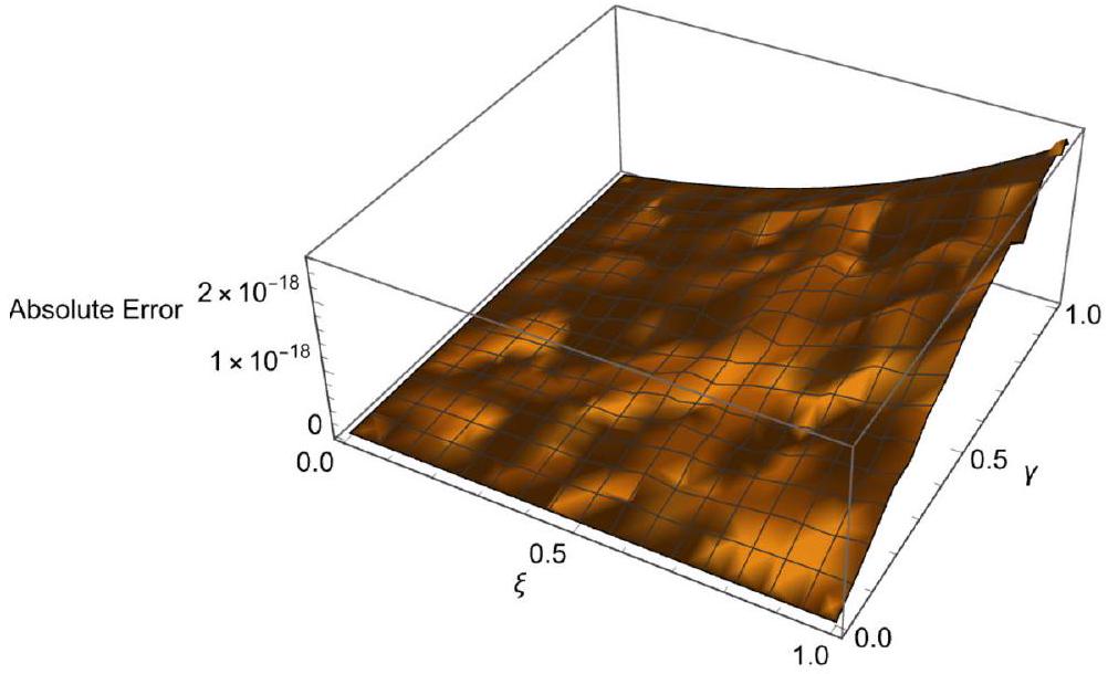
في الجدول 1، نقارن بين AEs لطريقة 3KMSCPs عندإلى طرق أخرى في [33،34]. تقدم الجدول 2 الأخطاء النظرية لقيم مختلفة من M. يوفر الجدول 3 الأخطاء المطلقة لمختلف و القيم عند. ل و معنوضح AEs التي تم إنشاؤها بواسطة طريقتنا في الشكل 1.
مثال 2 لـ، مع الدوائر المتكاملة والدوائر الأساسية المعطاة كما يلي:
الجدول 3 الأحداث الضائرة باستخدام طريقة (3KMSCPs) مع و إلى المثال 1
0
0.00
0.00
0.00
0.125
0.250
0.00
0.375
0.500
0.00
0.625
0.750
0.875
1.000
0.00
0.00
0.00
الشكل 1 الآثار الجانبية مع، و للمثال 1
الجدول 4 AE في، و للمثال 2
0.01
0.00
0.02
0.03
0.04
0.05
0.06
0.07
0.08
0.09
الحل الدقيق موضح في [35] كـ
الجدول 4 يعرض الأحداث الضائرة لـ، و يوضح الجدول 5 الأخطاء النظرية لقيم مختلفة من M. نقوم بتحليل الحد الأقصى للخطأ المطلق (MAE) بين طريقتنا في والطريقة في [35] عند مع و في الجدول 6. يمثل الجدول 7 أيضًا الأخطاء النظرية لقيم مختلفة من M. توضح الشكل 2 الفرق بين الحلول الدقيقة والتقريبية مع، ، و .
الجدول 5 الخطأ النظري AEs للتمرين 2 باستخدام طريقتنا
أيه إي
الجدول 6 فحص MAE للتمرين 2 لـ و
3KMSCPs ( )
الطريقة في [35] ( )
0.5
1.0
الجدول 7 الخطأ النظري AEs للتمرين 2 باستخدام طريقتنا
الشكل 2 التباين بين الحلول الدقيقة والحلول التقريبية لـ، و أكثر من المثال 2
مثال 3 لـ، مع الدوائر المتكاملة التالية ودوائر التبديل:
الحل التحليلي موضح في [25,35] كـ
نقارن بين النتائج التي تم الحصول عليها من خلال طريقتنا عندما نستفيد من مجموعة متنوعة من و لـ في الجدول 8. يقدم الجدول 9 الأخطاء النظرية لقيم مختلفة من M مع 0.5. الجدول 10 يقارن طريقتنا مع طرق أخرى [25،35] من خلال حساب MAEs عند، ، و تظهر الجدول 11 الأخطاء النظرية مع“، وقيم مختلفة من M. بالإضافة إلى ذلك، تقارن الجدول 12 3KMSCPs ( ) والطريقة
الجدول 8 مقارنة الآثار الجانبية بواسطة طريقة 3KMSCPs مع و للمثال 3
0.01
0.02
0.03
0.04
0.05
0.06
0.07
0.08
0.09
الجدول 9 الخطأ النظري AEs للتمرين 3 باستخدام طريقتنا
الجدول 10 مقارنة بين متوسطات الخطأ المطلق و لـ مثال 3 مع
3KMSCPs
طريقة في
طريقة في
0.5
1.0
1.5
–
الجدول 11 الخطأ النظري AEs للتمرين 3 باستخدام طريقتنا
أيه إي
0
الجدول 12 مقارنة بين MAEs لـ Ex. و
3KMSCPs
طريقة في
0.5
في [35] ( ) مع و للحصول على أقصى الأخطاء المطلقة. الجدول 13 يقدم الأخطاء النظرية لقيم مختلفة من، و تظهر الشكل 3 تأثير AE لـ، و .
الجدول 13 الخطأ النظري AEs للتمرين 3 باستخدام طريقتنا
أيه إي
0
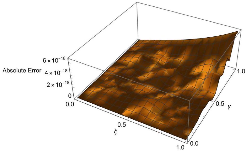
الشكل 3 توضيح رسومي لـ AE باستخدام، و للمثال 3
الجدول 14 متوسط الأخطاء المطلقة لمثال 4 مع
3KMSCPs ( )
الطريقة في [25] ( )
الطريقة في [36] ( )
1
2
٣
مثال 4 لـ، فإن الدوائر المتكاملة (ICs) والدوائر الأساسية (BCs) هي كما يلي:
الحل التحليلي موضح في [25، 36] كـ
يتم توضيح المقارنة في الجدول 14، حيث تظهر قيم الخطأ المطلق المتوسط بين 3KMSCPs ( ) وآخرون تم حسابها باستخدام، و تقدم الجدول 15 الأخطاء النظرية لقيم مختلفة من M ويوفر الجدول 16 نتائج MAE في، و لـالجدول 17 يوضح الأخطاء النظرية لقيم مختلفة من M،، و أرقام، و 8 توضح AEs لمختلف، و .
الجدول 15 الخطأ النظري AEs للتمرين 4 باستخدام طريقتنا
أيه إي
0.0147245
0
الجدول 16 متوسط الأخطاء المطلقة مع، و للمثال 4
0.0001
0.0002
0.0003
0.0004
0.0005
0.0006
0.0007
0.0008
0.0009
الجدول 17 الخطأ النظري AEs للتمرين 4 باستخدام طريقتنا
أيه إي
الشكل 4 AE مع، و للمثال 4
مثال 5 لـدع الدوائر المتكاملة والدوائر الأساسية تكون كما يلي:
الشكل 5 AE مع، و للمثال 4
الشكل 6 AE مع، و للمثال 4
الحل الدقيق موضح في [25,36] كالتالي
في الجدول 18، نقارن بين متوسطات الخطأ المطلق في حالات، و بين طريقة 3kMSCPs والطرق في [25، 36]. توضح الجدول 19 الأخطاء النظرية لقيم مختلفة من، و . مع ، وفي الجدول 20، نقوم بإدراج AEs بواسطة طريقة 3KMSCPs باستخدام القيم التالية:، ، و تقدم الجدول 21 الأخطاء النظرية مع قيم مختلفة من، و توضح الأشكال 9 و 10 سلوك AEs لـ و مع، و .
6 الاستنتاجات
في الدراسة الحالية، حصلنا على تقريبات عددية لمعادلات التلغراف الهايبرولية في بعد واحد وبعدين باستخدام طريقة 3KMSCPs من خلال الطرق الطيفية. الخطأ
الشكل 7 AE مع، و للمثال 4
الشكل 8 AE مع، و للمثال 4
الجدول 18 متوسط الأخطاء المطلقة للتمرين 5 مع، و
3KMSCPs ( )
الطريقة في [25] ( )
الطريقة في [36] ( )
1
2
٣
٥
الجدول 19 الخطأ النظري AEs للتمرين 5 باستخدام طريقتنا
أيه إي
0
0
تم تقييمه لضمان قابلية مقارنة النتائج، وتُعرض النتائج في كل من التنسيقات الجدولية والرسومية. أسفرت النتائج العددية عن أخطاء قريبة من الصفر. الـ
الجدول 20 AEs مع، و للمثال 5 بواسطة طريقة 3KMSCPs
0.0001
0.0002
0.0003
0.0004
0.0005
0.0006
0.0007
0.0008
0.0009
الجدول 21 الخطأ النظري AEs للتمرين 5 باستخدام طريقتنا
0
الشكل 9 AE مع، و للمثال 5
الشكل 10 AE مع، و للمثال 5
يثبت الخوارزم الحالي أنه أكثر فعالية في حل المعادلات التفاضلية الجزئية المعقدة وسهل التنفيذ.
مساهمات المؤلفين
لقد قبل جميع المؤلفين المسؤولية عن المحتوى الكامل لهذا المخطوط، ووافقوا على تقديمه إلى المجلة، وراجعوا جميع النتائج، ووافقوا على النسخة النهائية. قام SMS وYHY بتصميم وإجراء التجارب. طور SMS كود النموذج وأجرى المحاكاة. راجع ASM وEMA النص بالكامل. أعد YHY المخطوط بمساهمات من جميع المؤلفين المشاركين.
تمويل
تم توفير تمويل الوصول المفتوح من قبل هيئة تمويل العلوم والتكنولوجيا والابتكار (STDF) بالتعاون مع البنك المصري للمعرفة (EKB). لم يتلق المؤلفون أي دعم مالي للبحث.
توفر البيانات
لم يتم إنشاء أو تحليل أي مجموعات بيانات خلال الدراسة الحالية.
الإعلانات
المصالح المتنافسة
يعلن المؤلفون عدم وجود مصالح متنافسة.
تفاصيل المؤلف
قسم الرياضيات، كلية العلوم، جامعة حلوان، القاهرة 11795، مصر.قسم الرياضيات، كلية العلوم، جامعة القاهرة، الجيزة 12613، مصر.
تاريخ الاستلام: 18 نوفمبر 2024 تاريخ القبول: 22 ديسمبر 2024 تاريخ النشر على الإنترنت: 16 يناير 2025
References
Marin, M., Öchsner, A., Bhatti, M.M.: Some results in Moore-Gibson-Thompson thermoelasticity of dipolar bodies. Z. Angew. Math. Mech. 100(12), e202000090 (2020)
Sharma, S., Khator, S.: Power generation planning with reserve dispatch and weather uncertainties including penetration of renewable sources. Int. J. Smart Grid Clean Energy 10(4), 292-303 (2021)
Vlase, S., Marin, M., Scutaru, M.L., Munteanu, R.: Coupled transverse and torsional vibrations in a mechanical system with two identical beams. AIP Adv. 7(6), 065301 (2017)
Marin, M., Abbas, I., Kumar, R.: Relaxed Saint-Venant principle for thermoelastic micropolar diffusion. Struct. Eng. Mech. 51(4), 651-662 (2014)
Groza, G.H., Ali Khan, S.M., Pop, N.: Approximate solutions of boundary value problems for ODEs using Newton interpolating series. Carpath. J. Math. 25, 73-81 (2009)
Atta, A.G., Soliman, J.F., Elsaeed, E.W., Elsaeed, M.W., Youssri, Y.H.: Spectral collocation algorithm for the fractional Bratu equation via Hexic shifted Chebyshev polynomials. Comput. Methods Differ. Equ. (2024)
Youssri, Y.H., Hafez, R.M., Atta, A.G.: An innovative pseudo-spectral Galerkin algorithm for the time-fractional Tricomi-type equation. Phys. Scr. 99(10), 105238 (2024)
Atta, A.G., Abd-Elhameed, W.M., Youssri, Y.H.: Approximate collocation solution for the time-fractional Newell-Whitehead-Segel equation. J. Appl. Math. Comput. Mech. (2024)
Youssri, Y.H., Atta, A.G.: Radical Petrov-Galerkin approach for the time-fractional KdV-Burgers’ equation. Math. Comput. Appl. 29(6), 107 (2024)
Youssri, Y.H., Atta, A.G., Abu Waar, Z.Y., Moustafa, M.O.: Petrov-Galerkin method for small deflections in fourth-order beam equations in civil engineering. Nonlinear Eng. 13(1), 20240022 (2024)
Yassin, N.M., Aly, E.H., Atta, A.G.: Novel approach by shifted Schröder polynomials for solving the fractional Bagley-Torvik equation. Phys. Scr. (2024)
Youssri, Y.H., Abd-Elhameed, W.M., Mohamed, A.S., Sayed, S.M.: Generalized Lucas polynomial sequence treatment of fractional pantograph differential equation. Int. J. Appl. Comput. Math. 7, 1-16 (2021)
Youssri, Y.H., Sayed, S.M., Mohamed, A.S., Aboeldahab, E.M., Abd-Elhameed, W.M.: Modified Lucas polynomials for the numerical treatment of second-order boundary value problems. Comput. Methods Differ. Equ. 11(1), 12-31 (2023)
Youssri, Y.H., Abd-Elhameed, W.M., Sayed, S.M.: Generalized Lucas tau method for the numerical treatment of the one and two-dimensional partial differential heat equation. J. Funct. Spaces 2022(1), 3128586 (2022)
Sayed, S.M., Mohamed, A.S., Abo-Eldahab, E.M., Youssri, Y.H.: Legendre-Galerkin spectral algorithm for fractional-order BVPs: application to the Bagley-Torvik equation. Math. Syst. Sci. 2(1), 2733 (2024)
Ahmed, H.M., Youssri, Y.H., Abd-Elhameed, W.M.: Recursive and explicit formulas for expansion and connection coefficients in series of classical orthogonal polynomial products. Contemp. Math. 5(4), 4836-4873 (2024)
Youssri, Y.H., Ismail, M.I., Atta, A.G.: Chebyshev Petrov-Galerkin procedure for the time-fractional heat equation with nonlocal conditions. Phys. Scr. 99(1), 015251 (2023)
Pascal, H.: Pressure wave propagation in a fluid flowing through a porous medium and problems related to interpretation of Stoneley’s wave attenuation in acoustical well logging. Int. J. Eng. Sci. 24(9), 1553-1570 (1986)
Evans, D.J., Bulut, H.: The numerical solution of the telegraph equation by the alternating group explicit (age) method. Int. J. Comput. Math. 80(10), 1289-1297 (2003)
Jordan, P.M., Meyer, M.R., Puri, A.: Causal implications of viscous damping in compressible fluid flows. Phys. Rev. E 62(6), 7918 (2000)
Mohanty, R.K.: New unconditionally stable difference schemes for the solution of multi-dimensional telegraphic equations. Int. J. Comput. Math. 86(12), 2061-2071 (2009)
Kapoor, M.: Numerical solution of one-and two-dimensional hyperbolic telegraph equation via cubic-quartic hyperbolic B-spline DQM: a statistical validity. J. Math. Chem., 1-34 (2024)
Youssri, Y.H., Abd-Elhameed, W.M., Ahmed, H.M.: New fractional derivative expression of the shifted third-kind Chebyshev polynomials: application to a type of nonlinear fractional pantograph differential equations. J. Funct. Spaces 2022(1), 3966135 (2022)
Mazya, V.: Sobolev Spaces. Springer, Berlin (2013)
Magdy, E., Atta, A.G., Moatimid, G.M., Abd-Elhameed, W.M., Youssri, Y.H.: Enhanced fifth-kind Chebyshev polynomials Petrov-Galerkin algorithm for time-fractional Fokker-Planck equation. Int. J. Mod. Phys. C (2024)
Youssri, Y.H.: A new operational matrix of Caputo fractional derivatives of Fermat polynomials: an application for solving the Bagley-Torvik equation. Adv. Differ. Equ. 2017, 73, 1-17 (2017)
Atta, A.G., Abd-Elhameed, W.M., Moatimid, G.M., Youssri, Y.H.: Advanced shifted sixth-kind Chebyshev tau approach for solving linear one-dimensional hyperbolic telegraph type problem. Math. Sci. 17(4), 415-429 (2023)
Abdelghany, E.M., Abd-Elhameed, W.M., Moatimid, G.M., Youssri, Y.H., Atta, A.G.: A tau approach for solving time-fractional heat equation based on the shifted sixth-kind Chebyshev polynomials. Symmetry 15(3), 594 (2023)
Rainville, E.D.: Special Functions. Macmillan Co., New York (1960)
Saadatmandi, A., Dehghan, M.: Numerical solution of hyperbolic telegraph equation using the Chebyshev tau method. Numer. Methods Partial Differ. Equ. 26(1), 239-252 (2010)
El-Azab, M.S., El-Gamel, M.: A numerical algorithm for the solution of telegraph equations. Appl. Math. Comput. 190(1), 757-764 (2007)
Jiwari, R., Pandit, S., Mittal, R.C.: A differential quadrature algorithm for the numerical solution of the second-order one dimensional hyperbolic telegraph equation. Int. J. Nonlinear Sci. 13(3), 259-266 (2012)
Mittal, R.C., Bhatia, R.: A numerical study of two dimensional hyperbolic telegraph equation by modified B-spline differential quadrature method. Appl. Math. Comput. 244, 976-997 (2014)
ملاحظة الناشر
تظل شركة سبرينجر ناتشر محايدة فيما يتعلق بالمطالبات القضائية في الخرائط المنشورة والانتماءات المؤسسية.
Spectral framework using modified shifted Chebyshev polynomials of the third-kind for numerical solutions of one- and two-dimensional hyperbolic telegraph equations
Correspondence: youssri@cu.edu.eg Department of Mathematics, Faculty of Science, Cairo University, Giza 12613, Egypt
Full list of author information is available at the end of the article
Abstract
This investigation discusses a numerical approach to solving the hyperbolic telegraph equation in both one and two dimensions. Applying the Galerkin method is the basis of this approach. We use appropriate combinations of third-kind modified shifted Chebyshev polynomials (3KMSCPs) as basis functions to transform the governing partial differential equations into a collection of algebraic equations. Through spectral Galerkin techniques, we establish the convergence error to demonstrate that our algorithm is more effective and efficient. Five examples are examined to verify the effectiveness and resilience of the applied method by comparing errors and illustrating the results. Our results show that the current numerical solutions align closely with exact solutions. The current algorithm is simple to set up and is better suited to solving certain difficult partial differential equations.
Numerical solutions for boundary value problems (BVPs) and other real-life models (as, e.g., in [1-4]) play an important role in modern mathematics research. Computer systems are built by evaluating BVPs, computing numerical solutions, and determining convergent alternatives. Recently, various strategies for finding numerical answers have been proposed [5].
Spectral methods are numerical methods for handling differential equations [6-11], especially partial differential equations (PDEs). They vary from other numerical methods, such as finite difference and finite element methods, in that they depend on global basis functions and are derived from orthogonal polynomials to arrive at the approximate solution of a differential equation. Spectral methods have gained popularity in scientific computing due to their ability to produce extremely accurate solutions with few degrees of
freedom, even when the solution is smooth. This makes spectral methods ideal for problems including quantum mechanics, fluid dynamics, and a wide range of other fields that demand precise numerical solutions to PDEs. The main benefit of spectral methods is the exponential convergence over smooth problems. While finite difference methods typically converge at a polynomial rate, spectral methods converge much faster, especially for smooth solutions. The calculation error decreases as , where represents the number of basis functions applied, and is a constant. This means that with only a single basis function, spectral methods can yield greatly accurate approximations of the solution. There are generally four spectral methods: Galerkin, tau, collocation (pseudospectral), and Fourier spectral methods (a specific kind of collocation). The choice of the Galerkin, tau, or collocation methods is determined by the specific problem, the boundary conditions, and the smoothness of the calculated solution. Each method achieves great accuracy, frequently with exponential convergence; for more detail about the spectral methods, see [12-17].
Chebyshev polynomials are a group of orthogonal polynomials that are useful in numerical analysis, approximations theory, and differential equations. These polynomials are named after the Russian mathematician Pafnuty Chebyshev and are commonly employed due to their helpful qualities, which include minimizing the impacts of Runge’s phenomenon in the interpolation of polynomials and achieving quick convergence in approximations. Chebyshev polynomials have developed as a highly effective approximation for numerical analysis with orthogonality restrictions. They are essential in approximation theory because of their minimality qualities and their links to the Laurent and Fourier series with continuous and discrete orthogonality function spaces [18, 19].
The hyperbolic partial differential equations that describe structural vibrations serve as the foundation for fundamental equations in atomic physics. The telegraph equation is used in the study of wave phenomena and electrical signal propagation along a transmission line wire [20,21]. The equation of viscous Maxwell fluids governs processes such as acoustic wave propagation in Darcy-type porous media and parallel flows. See [22, 23] for more detail. Biologists use these equations to investigate pulsed blood flow in arteries and 1D random migration of bugs along a hedge [24]. In this research, we are interested in establishing an algorithm to find a semianalytic solution to the hyperbolic telegraph equations.
Hyperbolic telegraph equation in one dimension [25]
with the initial conditions (ICs) for :
and the boundary conditions (BCs) for :
Hyperbolic telegraph equation in two dimensions [25]
with ICs for :
and BCs for and :
where , and are given functions.
The basic framework of the current study: Sect. 2 introduces how to convert the nonhomogeneous boundary conditions to homogeneous ones. In Sect. 3, we discuss an outline of the third-kind shifted and modified shifted Chebyshev polynomials. We focus on the convergence and error analysis and construct a new algorithm for solving hyperbolic telegraph equations in Sect. 4. Finally, we solve hyperbolic telegraph equations by comparing our 3KMSCPs method to other research in Sect. 5.
2 The conversion of the nonhomogeneous conditions to homogeneous ones
We employ homogeneous initial and boundary conditions in our basis function. Hence we need to convert the nonhomogeneous conditions to homogeneous ones via the following transformation.
1D hyperbolic telegraph equations. Let
With the aid of the converter equation
Equation (1) converts into
which in turn is simplified to
where
with the ICs
and the BCs
2D hyperbolic telegraph equations. Let the aid converter equation be given as
Using it and applying the ICs and BCs, we get
Using Equations (14) and (15) in Eq. (4), the latter becomes
which can be simplified to
where
Applying the ICs and BCs, we can express as
based on ICs for ,
and BCs for and ,
3 Outline of the 3KMSCPs method
In this section, we review 3KCPs, 3KSCPs, 3KMSCPs, power forms, and some useful relations.
3.1 3rd-kind of Chebyshev polynomials (3KCPs)
Chebyshev polynomials of the third kind are well known in the region and have the following recurrence relation [26]:
with
The zeros of the recurrence relation (22) are supplied as
The Rodrigues representation of the third-kind Chebyshev polynomials is denoted in [26] by
In addition, by noting that the third-kind Chebyshev polynomials is a particular case of Jacobi polynomials, it is easy to demonstrate that
where is the hypergeometric function of order .
The power (analytical) form of 3KCPs is [26]
Another analytical form for 3KCPs is given in [26] by
where is the lowest integer greater than or equal to .
The polynomials are orthogonal on in terms of the inner product with weight function :
with and the Kronecker delta determined by
3.2 3rd-kind of shifted Chebyshev polynomials (3KSCPs)
The range is generally more convenient to utilize than the range . We can convert the independent variable into the variable in by using the transformation , which gives 3 KSCPs , of degree .
These polynomials are orthogonal along the interval :
with the weight function . They can also be defined by the recurrence relation [26]
with Jacobi polynomials .
Theorem 1 The polynomials are orthogonal on with respect to the weight function :
Proof To begin, we insert and into the left-hand side, simplify the results, and then integrate the result from 0 to 1 :
Theorem 2 The polynomials , are orthogonal with respect to the weight function :
Proof Follow the same steps as in Theorem 1.
The approximate solution for 1D hyperbolic telegraph equations. Consider the pair of basis functions and . Assume the following two spaces:
where the Sobolev space , with , is defined as
The associated norm is given by
and the inner product in is defined as
For more detail, we refer to the book [27].
Now we obtain the approximate solution of Eq. (1) by integrating both sides twice for :
where
Also, we can obtain the approximate solution from Eq. (10), which is Eq. (1) after converting it to homogeneous BCs and ICs. The result is as follows:
where
The approximate solution of in Eq. (10) is denoted by
where and are defined in Eq. (35). Substitute into Eq. (10) to get the residual
Applying the Galerkin method to the last equation, we get
where
and the weight function is defined as
We arrange Eq. (46) as
The following expression is identical to (50):
Having the unknown expansion coefficients , Eq. (51) provides a nonlinear system of algebraic equations of dimension that can be handled by a suitable solver.
The following theorem defines , and , and is given by
Theorem 3 The elements and are
Proof Using the orthogonality relation of and the power form of , we can derive :
We leverage the orthogonality property and Eq. (35) to derive :
We employ the orthogonality property to derive the elements , and :
where yield the Jacobi polynomials.
The elements of are given as
and as
The approximate solution for 2D hyperbolic telegraph equations. We provide an approximate solution in the form
Integrating twice both sides of Eq. (17) with respect to , we get the residual of Eq. (17):
Now we substitute into Eq. (60) to get the approximate solution
Then, employing the Galerkin method on Eq. (61), we have
where
Arranging Eq. (62), we have
To simplify the last equation, we denote
and . Then we can rewrite Eq. (64) as
with
and the elements , and are given in Theorem 3. Then the unknown coefficients in Eq. (65) from that equation, which has a nonlinear system of algebraic equations of dimension , can be determined by any algebraic method.
4 Convergence analysis
In this section, we study the convergence of the employed basis functions. The Mathematica program estimates the following values.
Lemma 1 For , and , the polynomials and fulfill that following inequalities:
Proof Applying the recurrence relation (32) for as in Eq. (67) and using the triangle inequality, we get
To prove the second relation in Eq. (67), using the definition of in Eq. (35) and the relation of in Eq. (67), we derive
This concludes the proof of the lemma.
Theorem 4 Let and be attached to the space , and . Let and be enlarged as
Then
Proof To prove this theorem, follow the steps outlined in [28-31].
Theorem 5 With and , we have the following estimate of the absolute error:
Proof Using the definition of the absolute error, Lemma 1, and Theorem 4, we get
Utilizing the properties of the exponential function, we obtain
where , and are, respectively, the upper incomplete gamma, gamma, and lower incomplete gamma functions. For more information about them, we refer to [32].
Theorem6 With , and , we have the following estimate of the absolute error in two dimensions:
Algorithm 1 Solving Hyperbolic Telegraph Equations Using Spectral 3KMSCPs Method
Input Set constants $epsilon$ and $rho$ for the hyperbolic telegraph equation.
Put the value of $M$.
Step 1. Convert nonhomogeneous boundary conditions to homogeneous conditions:
- Define transformation functions (e.g., $E(xi, eta)$ for 1D and $S(xi, Upsilon, eta)$ for 2D)
to handle boundary terms.
- Express the hyperbolic telegraph equation using the transformed function $omega$
with homogeneous boundary conditions.
Step 2. Construct the basis functions of the 3KMSCPs method
$varphi_{i}(xi)=xi(1-xi) Im_{i}^{star}(xi)$ and $psi_{j}(eta)=V_{j}^{left(-frac{1}{2}, frac{1}{2}right)}left(frac{2 eta}{T}-1right)$ for problems (10) and (17).
Step 3. Express the solution as a series expansion:
- Represent the approximate solutions $U(xi, eta)$ and $U(xi, Upsilon, eta)$ as finite series
$U(xi, eta)=sum_{i=0}^{M} sum_{j=0}^{M} c_{i j} varphi_{i}(xi) psi_{j}(eta)$,
$U(xi, Upsilon, eta)=sum_{j=0}^{M} sum_{l=0}^{M} sum_{i=0}^{M} c_{i l j} varphi_{i}(xi) varphi_{l}(Upsilon) psi_{j}(eta)$.
- Determine the coefficients $c_{i j}$ and $c_{i l j}$ applying the spectral Galerkin method.
Step 4. Apply the spectral Galerkin method:
- Substitute the series expansion into the transformed hyperbolic telegraph
equation.
- Minimize the residuals $Z(xi, eta)$ and $Z(xi, Upsilon, eta)$ by ensuring the orthogonality
with the basis functions, leading to a system of algebraic equations in terms
of the coefficients $c_{i j}$ and $c_{i l j}$.
Step 5. Solve the algebraic system equations:
Solve the resulting system using an appropriate numerical method, such as
Gaussian elimination or an iterative solver.
Output Display the computed solution $U(xi, eta)$ and $U(xi, Upsilon, eta)$ to provide errors, which
exist in their definition in Step 3.
Proof Following the same steps as in the proof of Theorem 5, but in 2D, we have the final relations
5 Solving hyperbolic telegraph problems in 1D and 2D
In this section, we evaluate one- and two-dimensional hyperbolic telegraph problems using the 3KMSCPs method to quantify the absolute error (AE) and make helpful comparisons. All examples were computed using Mathematica version 14. The basic equation discussed in these cases is Eq. (1).
Example 1 For the function , with the ICs and BCs
the exact solution is given in [33,34] as
With , we get the approximate solution
with residual (51) given by
Applying the spectral Galerkin method, the corresponding algebraic system of equations is
Table 1 AEs for Ex. 1 with
3KMSCPs ( )
Method in [33] ( )
Method in [34]
0
0.00
0.00
0.00
0.125
0.250
0.375
0.500
0.625
0.750
0.875
1.000
0.00
0.00
Table 2 The theoretical error AEs for Ex. 1 using our method
1.186703056
with the coefficients , and -0.00313475 . Finally, the approximate solution is
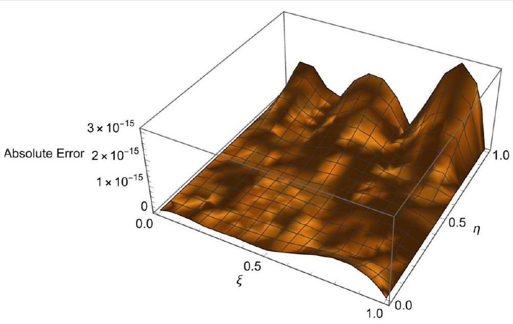
In Table 1, we compare AEs of the 3KMSCPs method at to other methods in [33,34]. Table 2 presents the theoretical errors for different values of M . Table 3 provides the absolute errors for various and values at . For and with , we illustrate AEs generated by our method in Fig. 1.
Example 2 For , with the ICs and BCs given as follows:
Table 3 AEs using (3KMSCPs) method with and to Ex. 1
0
0.00
0.00
0.00
0.125
0.250
0.00
0.375
0.500
0.00
0.625
0.750
0.875
1.000
0.00
0.00
0.00
Figure 1 AEs with , and for Ex. 1
Table 4 AE at , and for Ex. 2
0.01
0.00
0.02
0.03
0.04
0.05
0.06
0.07
0.08
0.09
The exact solution is given in [35] as
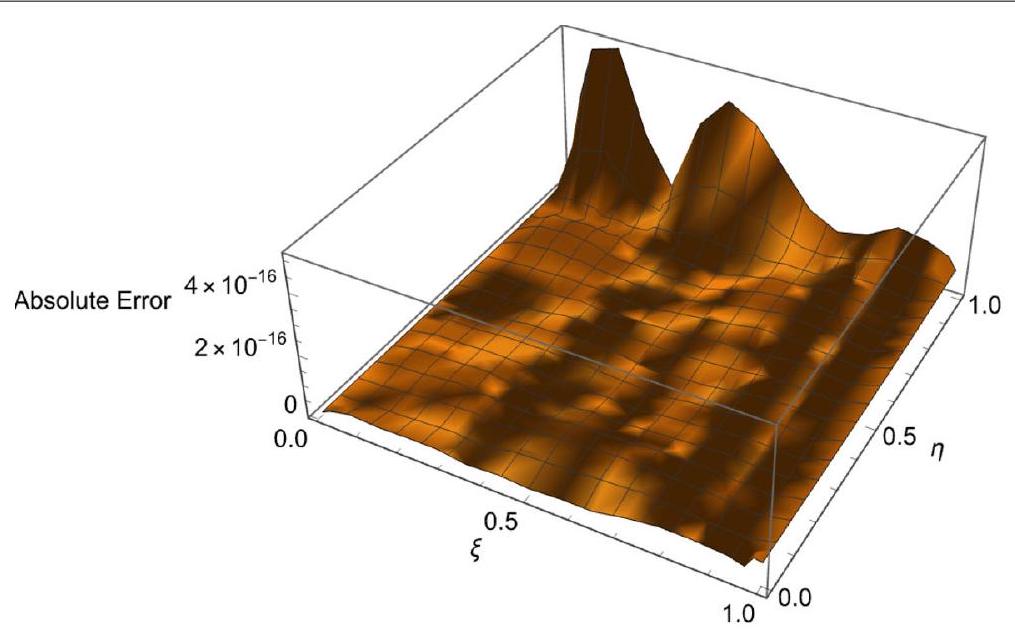
Table 4 presents AEs for , and . Tab. 5 shows the theoretical errors for different values of M. We analyze the maximum absolute error (MAE) between our method at and the method in [35] at with and in Table 6. Tab. 7 also represents the theoretical errors for different values of M. Figure 2 demonstrates the difference between exact and approximate solutions with , , and .
Table 5 The theoretical error AEs for Ex. 2 using our method
AEs
Table 6 Examination of MAE for Ex. 2 for and
3KMSCPs ( )
Method in [35] ( )
0.5
1.0
Table 7 The theoretical error AEs for Ex. 2 using our method
Figure 2 The variation between exact and approximate solutions for , and over Ex. 2
Example 3 For , with the following ICs and BCs:
The analytical solution is given in [25,35] as
We compare the AEs obtained via our method when we harness a variety of and for in Tab. 8. Table 9 presents the theoretical errors for different values of M with 0.5 . Table 10 compares our method with others [25,35] by computing MAEs at , , and . Tab. 11 shows the theoretical errors with , and different values of M. In addition, Tab. 12 compares 3KMSCPs ( ) and the method
Table 8 Comparison of AEs by 3KMSCPs method with and for Ex. 3
0.01
0.02
0.03
0.04
0.05
0.06
0.07
0.08
0.09
Table 9 The theoretical error AEs for Ex. 3 using our method
Table 10 Comparison of MAEs for and for Ex. 3 with
3KMSCPs
Method in
Method in
0.5
1.0
1.5
–
Table 11 The theoretical error AEs for Ex. 3 using our method
AEs
0
Table 12 Comparison of MAEs for Ex. and
3KMSCPs
Method in
0.5
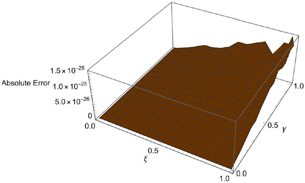
in [35] ( ) with and to obtain the maximum absolute errors. Table 13 presents the theoretical errors for different values of , and . Figure 3 shows the action of AE for , and .
Table 13 The theoretical error AEs for Ex. 3 using our method
AEs
0
Figure 3 Graphical illustration of AE using , and for Ex. 3
Table 14 MAEs for Ex. 4 with
3KMSCPs ( )
Method in [25] ( )
Method in [36] ( )
1
2
3
Example 4 For , the ICs and BCs are as follows:
The analytical solution is given in [25, 36] as
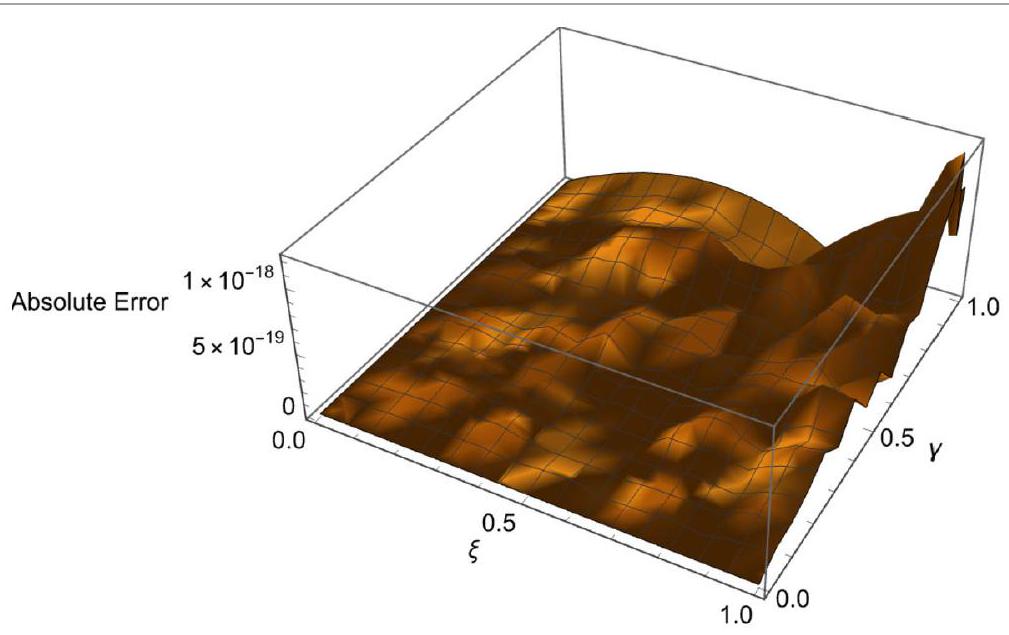
The comparison is demonstrated in Table 14, the MAEs between 3KMSCPs ( ) and others were calculated using , and . Tab. 15 presents the theoretical errors for different values of M and . Table 16 provides the MAE findings at , and for . Table 17 expounds the theoretical errors for different values of M , , and . Figures , and 8 depict the AEs for various , and .
Table 15 The theoretical error AEs for Ex. 4 using our method
AEs
0.0147245
0
Table 16 The MAEs with , and for Ex. 4
0.0001
0.0002
0.0003
0.0004
0.0005
0.0006
0.0007
0.0008
0.0009
Table 17 The theoretical error AEs for Ex. 4 using our method
AEs
Figure 4 AE with , and for Ex. 4
Example 5 For , let the ICs and BCs be as follows:
Figure 5 AE with , and for Ex. 4
Figure 6 AE with , and for Ex. 4
The exact solution is given in [25,36] as
In Table 18, we compare the MAEs in cases of , and between the 3kMSCPs method and the methods in [25, 36]. Table 19 illustrates the theoretical errors for different values of , and . With , and 8, in Table 20, we list the AEs by the 3KMSCPs method using the following values: , , and . Table 21 presents the theoretical errors with different values of , and . Figures 9 and 10 depict the behavior of the AEs for and with , and .
6 Conclusions
In the current study, we obtained numerical approximations for 1D and 2D hyperbolic telegraph equations using the 3KMSCPs method through spectral methods. The error
Figure 7 AE with , and for Ex. 4
Figure 8 AE with , and for Ex. 4
Table 18 The MAEs for Ex. 5 with , and
3KMSCPs ( )
Method in [25] ( )
Method in [36] ( )
1
2
3
5
Table 19 The theoretical error AEs for Ex. 5 using our method
AEs
0
0
was evaluated to ensure the comparability of results, and the findings are presented in both tabular and graphical formats. The numerical results yielded errors close to zero. The
Table 20 The AEs with , and for Ex. 5 by 3KMSCPs method
0.0001
0.0002
0.0003
0.0004
0.0005
0.0006
0.0007
0.0008
0.0009
Table 21 The theoretical error AEs for Ex. 5 using our method
0
Figure 9 AE with , and for Ex. 5
Figure 10 AE with , and for Ex. 5
current algorithm proves more effective for solving complex partial differential equations and is straightforward to implement.
Author contributions
All authors have accepted responsibility for the entire content of this manuscript, consented to its submission to the journal, reviewed all results, and approved the final version. SMS and YHY designed and conducted the experiments. SMS developed the model code and performed the simulations. ASM and EMA reviewed the entire text. YHY prepared the manuscript with contributions from all co-authors.
Funding
Open access funding provided by The Science, Technology & Innovation Funding Authority (STDF) in cooperation with The Egyptian Knowledge Bank (EKB). The authors received no financial support for the research.
Data Availability
No datasets were generated or analysed during the current study.
Declarations
Competing interests
The authors declare no competing interests.
Author details
Department of Mathematics, Faculty of Science, Helwan University, Cairo 11795, Egypt. Department of Mathematics, Faculty of Science, Cairo University, Giza 12613, Egypt.
Received: 18 November 2024 Accepted: 22 December 2024 Published online: 16 January 2025
References
Marin, M., Öchsner, A., Bhatti, M.M.: Some results in Moore-Gibson-Thompson thermoelasticity of dipolar bodies. Z. Angew. Math. Mech. 100(12), e202000090 (2020)
Sharma, S., Khator, S.: Power generation planning with reserve dispatch and weather uncertainties including penetration of renewable sources. Int. J. Smart Grid Clean Energy 10(4), 292-303 (2021)
Vlase, S., Marin, M., Scutaru, M.L., Munteanu, R.: Coupled transverse and torsional vibrations in a mechanical system with two identical beams. AIP Adv. 7(6), 065301 (2017)
Marin, M., Abbas, I., Kumar, R.: Relaxed Saint-Venant principle for thermoelastic micropolar diffusion. Struct. Eng. Mech. 51(4), 651-662 (2014)
Groza, G.H., Ali Khan, S.M., Pop, N.: Approximate solutions of boundary value problems for ODEs using Newton interpolating series. Carpath. J. Math. 25, 73-81 (2009)
Atta, A.G., Soliman, J.F., Elsaeed, E.W., Elsaeed, M.W., Youssri, Y.H.: Spectral collocation algorithm for the fractional Bratu equation via Hexic shifted Chebyshev polynomials. Comput. Methods Differ. Equ. (2024)
Youssri, Y.H., Hafez, R.M., Atta, A.G.: An innovative pseudo-spectral Galerkin algorithm for the time-fractional Tricomi-type equation. Phys. Scr. 99(10), 105238 (2024)
Atta, A.G., Abd-Elhameed, W.M., Youssri, Y.H.: Approximate collocation solution for the time-fractional Newell-Whitehead-Segel equation. J. Appl. Math. Comput. Mech. (2024)
Youssri, Y.H., Atta, A.G.: Radical Petrov-Galerkin approach for the time-fractional KdV-Burgers’ equation. Math. Comput. Appl. 29(6), 107 (2024)
Youssri, Y.H., Atta, A.G., Abu Waar, Z.Y., Moustafa, M.O.: Petrov-Galerkin method for small deflections in fourth-order beam equations in civil engineering. Nonlinear Eng. 13(1), 20240022 (2024)
Yassin, N.M., Aly, E.H., Atta, A.G.: Novel approach by shifted Schröder polynomials for solving the fractional Bagley-Torvik equation. Phys. Scr. (2024)
Youssri, Y.H., Abd-Elhameed, W.M., Mohamed, A.S., Sayed, S.M.: Generalized Lucas polynomial sequence treatment of fractional pantograph differential equation. Int. J. Appl. Comput. Math. 7, 1-16 (2021)
Youssri, Y.H., Sayed, S.M., Mohamed, A.S., Aboeldahab, E.M., Abd-Elhameed, W.M.: Modified Lucas polynomials for the numerical treatment of second-order boundary value problems. Comput. Methods Differ. Equ. 11(1), 12-31 (2023)
Youssri, Y.H., Abd-Elhameed, W.M., Sayed, S.M.: Generalized Lucas tau method for the numerical treatment of the one and two-dimensional partial differential heat equation. J. Funct. Spaces 2022(1), 3128586 (2022)
Sayed, S.M., Mohamed, A.S., Abo-Eldahab, E.M., Youssri, Y.H.: Legendre-Galerkin spectral algorithm for fractional-order BVPs: application to the Bagley-Torvik equation. Math. Syst. Sci. 2(1), 2733 (2024)
Ahmed, H.M., Youssri, Y.H., Abd-Elhameed, W.M.: Recursive and explicit formulas for expansion and connection coefficients in series of classical orthogonal polynomial products. Contemp. Math. 5(4), 4836-4873 (2024)
Youssri, Y.H., Ismail, M.I., Atta, A.G.: Chebyshev Petrov-Galerkin procedure for the time-fractional heat equation with nonlocal conditions. Phys. Scr. 99(1), 015251 (2023)
Pascal, H.: Pressure wave propagation in a fluid flowing through a porous medium and problems related to interpretation of Stoneley’s wave attenuation in acoustical well logging. Int. J. Eng. Sci. 24(9), 1553-1570 (1986)
Evans, D.J., Bulut, H.: The numerical solution of the telegraph equation by the alternating group explicit (age) method. Int. J. Comput. Math. 80(10), 1289-1297 (2003)
Jordan, P.M., Meyer, M.R., Puri, A.: Causal implications of viscous damping in compressible fluid flows. Phys. Rev. E 62(6), 7918 (2000)
Mohanty, R.K.: New unconditionally stable difference schemes for the solution of multi-dimensional telegraphic equations. Int. J. Comput. Math. 86(12), 2061-2071 (2009)
Kapoor, M.: Numerical solution of one-and two-dimensional hyperbolic telegraph equation via cubic-quartic hyperbolic B-spline DQM: a statistical validity. J. Math. Chem., 1-34 (2024)
Youssri, Y.H., Abd-Elhameed, W.M., Ahmed, H.M.: New fractional derivative expression of the shifted third-kind Chebyshev polynomials: application to a type of nonlinear fractional pantograph differential equations. J. Funct. Spaces 2022(1), 3966135 (2022)
Mazya, V.: Sobolev Spaces. Springer, Berlin (2013)
Magdy, E., Atta, A.G., Moatimid, G.M., Abd-Elhameed, W.M., Youssri, Y.H.: Enhanced fifth-kind Chebyshev polynomials Petrov-Galerkin algorithm for time-fractional Fokker-Planck equation. Int. J. Mod. Phys. C (2024)
Youssri, Y.H.: A new operational matrix of Caputo fractional derivatives of Fermat polynomials: an application for solving the Bagley-Torvik equation. Adv. Differ. Equ. 2017, 73, 1-17 (2017)
Atta, A.G., Abd-Elhameed, W.M., Moatimid, G.M., Youssri, Y.H.: Advanced shifted sixth-kind Chebyshev tau approach for solving linear one-dimensional hyperbolic telegraph type problem. Math. Sci. 17(4), 415-429 (2023)
Abdelghany, E.M., Abd-Elhameed, W.M., Moatimid, G.M., Youssri, Y.H., Atta, A.G.: A tau approach for solving time-fractional heat equation based on the shifted sixth-kind Chebyshev polynomials. Symmetry 15(3), 594 (2023)
Rainville, E.D.: Special Functions. Macmillan Co., New York (1960)
Saadatmandi, A., Dehghan, M.: Numerical solution of hyperbolic telegraph equation using the Chebyshev tau method. Numer. Methods Partial Differ. Equ. 26(1), 239-252 (2010)
El-Azab, M.S., El-Gamel, M.: A numerical algorithm for the solution of telegraph equations. Appl. Math. Comput. 190(1), 757-764 (2007)
Jiwari, R., Pandit, S., Mittal, R.C.: A differential quadrature algorithm for the numerical solution of the second-order one dimensional hyperbolic telegraph equation. Int. J. Nonlinear Sci. 13(3), 259-266 (2012)
Mittal, R.C., Bhatia, R.: A numerical study of two dimensional hyperbolic telegraph equation by modified B-spline differential quadrature method. Appl. Math. Comput. 244, 976-997 (2014)
Publisher’s Note
Springer Nature remains neutral with regard to jurisdictional claims in published maps and institutional affiliations.
Submit your manuscript to a SpringerOpen journal and benefit from: