III. استخدام كتل العناقيد وأشعاعها ودينامياتها لإنشاء كتالوج منظم للعناقيد المفتوحة
إميلي ل. هانتوسابين ريفرتالمرصد الوطني، مركز الفلك بجامعة هايدلبرغ، كونيغشتول 12، 69117 هايدلبرغ، ألمانياالبريد الإلكتروني: ehunt@lsw.uni-heidelberg.de
استلم في 17 نوفمبر 2023؛ قبل في 5 مارس 2024
الملخص
السياق. لقد انفجر تعداد العناقيد المفتوحة في الحجم بفضل بيانات من قمر Gaia الصناعي. ومع ذلك، من المحتمل أن العديد من هذه العناقيد المبلغ عنها ليست مرتبطة جاذبيًا، مما يجعل تعداد العناقيد المفتوحة غير عملي للعديد من التطبيقات العلمية. الأهداف. نهدف إلى اختبار طرق مختلفة مدفوعة جسديًا للتمييز بين العناقيد المرتبطة وغير المرتبطة، باستخدامها لإنشاء كتالوج منظم للعناقيد النجمية. الطرق. قمنا باشتقاق كتل فوتومترية مصححة من حيث الاكتمال لـ 6956 عنقودًا من عملنا السابق. ثم استخدمنا هذه الكتل لحساب حجم سطح روش لهذه العناقيد (نصف قطر جاكوب) وتمييز بين العناقيد المرتبطة وغير المرتبطة. النتائج. نجد أن فقطمن العناقيد في كتالوجنا السابق متوافقة مع العناقيد المفتوحة المرتبطة، مما ينخفض إلى مجردالعناقيد ضمن 250 فرسخ فلكي. يحتوي كتالوجنا على 3530 عنقود مفتوح في عينة ذات جودة عالية مقطوعة بشكل أقوى. تظهر المجموعات المتحركة في عينتنا اتجاهات مختلفة في حجمها كدالة للعمر والكتلة، مما يشير إلى أنها غير مرتبطة وتخضع لعمليات ديناميكية مختلفة. تشكل قياسات كتلة العناقيد لدينا أكبر كتالوج لكتل عناقيد درب التبانة حتى الآن، والذي نستخدمه أيضًا لأغراض علمية أخرى. أولاً، استنتجنا حد الاكتمال المعتمد على الكتلة لعد العناقيد المفتوحة، مما يظهر أن العد مكتمل ضمن 1.8 كيلوبارسيك فقط للأجسام الأثقل من. بعد ذلك، قمنا باشتقاق دالة العمر والكتلة المصححة للاكتمال لكتالوج العناقيد المفتوحة لدينا، بما في ذلك تقدير أن مجرة درب التبانة تحتوي على إجمالي العناقيد المفتوحة، فقطالتي تعرف حاليًا. أخيرًا، نوضح أن معظم العناقيد المفتوحة لها دوال كتلة متوافقة مع دالة الكتلة الأولية لكروب. الاستنتاجات. نوضح أنصاف أقطار جاكوبى للتمييز بين العناقيد النجمية المرتبطة وغير المرتبطة، وننشر كتالوجًا محدثًا للعناقيد النجمية مع الكتل وتصنيفات محسّنة للعناقيد.
الكلمات الرئيسية. العناقيد المفتوحة والجمعيات: عام – الطرق: تحليل البيانات – الفهارس – علم الفلك القياسي
1. المقدمة
أحدثت بيانات الأقمار الصناعية غايا ثورة كاملة في إحصاء العناقيد المفتوحة (OCs) (كانت غودين 2022). منذ أول إصدار كامل لبيانات غايا (براون وآخرون 2018)، تم إحراز تقدم في العديد من جوانب الإحصاء، بما في ذلك استبعاد العديد من العناقيد المفتوحة التي تم الإبلاغ عنها قبل غايا كأشكال نجمية (كانت غودين وأندرس 2020، بياتي وآخرون 2023، هانت وريفيرت 2021، 2023)، واكتشاف العديد من الآلاف من الأجسام الجديدة بفضل قياسات غايا الدقيقة (مثل ليو وبانغ 2019؛ كاسترو-جينارد وآخرون 2020)، وتحديد معلمات العناقيد بدقة أعلى مما كان ممكنًا سابقًا (مثل بوسيني وآخرون 2019، كانت غودين وآخرون 2020). ومع ذلك، لا يزال إحصاء العناقيد المفتوحة بحاجة إلى تحسين، حيث تكمن المشكلة الرئيسية في أن التعريفات الرصدية الحالية للعناقيد المفتوحة لا تبدو قوية بما يكفي لتمييزها عن المجموعات المتحركة غير المرتبطة (MGs) (هانت وريفيرت 2023).
تحسن كانت-غودين وأندرس (2020) على أول كتالوج رئيسي لمجموعات النجوم المفتوحة في عصر غايا، (كانت-غودين وآخرون 2018)، من خلال البحث عن مجموعات نجوم مفتوحة إضافية في بيانات غايا واستخدام
مجموعة من المعايير الرصدية للتمييز بين التجمعات النجمية المحتملة والأسترزمات. معاييرهم كالتالي: أولاً، يجب أن يكون التجمع النجمي المرشح كثافة واضحة، بما في ذلك أنه يحتوي على ما لا يقل عن عشرة نجوم أعضاء تقريبًا؛ ثانيًا، يجب أن يكون لديه مخطط لون-قدر (CMD) يتبع خط إيزوكرون واضح، مما يشير إلى أن التجمع المعين هو مجموعة من النجوم تتطور معًا بنفس العمر والتركيب الكيميائي؛ وأخيرًا، يجب أن يمر التجمع النجمي المرشح بمعايير تميز الأسترزمات التي لا يمكن أن تكون مرتبطة جاذبيًا من التجمعات النجمية المحتملة المرتبطة: وهي، نصف قطر وسطي.أقل من 15 في المئة، وتشتت الحركة المناسبة الذي يتوافق مع تشتت السرعة الداخلية أقل من (أو للمجموعات البعيدة حيث تكون عدم اليقين في قياسات غايا هي السائدة.
تعتبر المعايير المتعلقة بكثافة (أو عدد النجوم) وجودة CMD لمرشح العنقود المفتوح ممارسة شائعة في الأدبيات. على سبيل المثال، يتطلب Froebrich وآخرون (2007)، وCantat-Gaudin وآخرون (2019)، وHunt & Reffert (2021) (المشار إليه فيما بعد بالورقة I) أن يكون المرشح لعنقود جديد كثافة واضحة، بينما تعتبر أعمال مثل Platais وآخرون (1998)، وCastro-Ginard وآخرون (2018)، وLiu & Pang (2019) أمثلة على الأعمال التي تستخدم CMDs للعنقود للتحقق من صحة الكائنات الجديدة المرشحة. كما تم اعتماد معايير Cantat-Gaudin & Anders (2020) بشأن إمكانية أن يكون العنقود مرتبطًا في الأدبيات، مع أعمال مثل Hunt &
ريفيرت (2021) وكاسترو-جينارد وآخرون (2022) يستخدمونها للتحقق من صحة مرشحين جدد للمواد العضوية.
في Hunt & Reffert (2023) (المشار إليه فيما بعد بـ Paper II)، استخدمنا بيانات Gaia DR3 (تعاون Gaia وآخرون 2023) لإنشاء كتالوج كبير ومتجانس لمجموعات النجوم. ومع ذلك، على الرغم من أن منهجيتنا كانت تهدف في الأصل إلى اكتشاف OCs فقط، فإن العديد من المجموعات التي اكتشفناها تبدو MGs، وغالبًا ما تكون لها توزيعات نجمية متناثرة أو ‘مسطحة’ – على عكس المظهر المتجمع لـ OCs المرتبطة تقليديًا مثل الثريا. العديد من MGs المشتبه بها التي اكتشفناها تتماشى مع كونها مجموعات سكانية فردية من النجوم المتطورة بشكل مشترك بناءً على مصنف CMD الخاص بنا في Paper II، ولا يزال معظم MGs التي اكتشفناها تمر بالمعايير الرصدية المتعلقة بارتباط OC المقترحة في CantatGaudin & Anders (2020). في Paper II، اقترحنا أن هذه المعايير متساهلة جدًا لتصنيف العديد من مجموعات النجوم المتناثرة التي يمكننا اكتشافها بالقرب من الشمس بدقة. إن عدم القدرة على التمييز بدقة بين المجموعات المرتبطة وغير المرتبطة يحد من الاستخدام العلمي للكتالوجات مثل الكتالوج الموجود في Paper II، مع احتمال أن تكون نسبة كبيرة من محتوى الكتالوج MGs – خاصة ضمن حوالي 1 كيلوبارسيك من الشمس.
في هذا العمل، نهدف إلى إنشاء طريقة جديدة للتمييز بين العناقيد المرتبطة وغير المرتبطة، مستفيدين من العلاقة بين الكتلة ونصف قطر جاكوبى لعناقيد الجاذبية الذاتية. من خلال هذه الطريقة، نهدف إلى تصنيف جميع الأجسام في الورقة الثانية إلى أجسام مرتبطة وغير مرتبطة، بالإضافة إلى إظهار قابلية تطبيق هذه الطريقة على الدراسات المستقبلية لعناقيد درب التبانة، مثل البيانات القادمة مثل Gaia DR4. أولاً، نقدم نظرة عامة على بعض النظرية الأساسية في القسم 2. في القسم 3، نوضح كيفية حساب كتل العناقيد وأشعاعها، بما في ذلك كيفية تصحيح تأثيرات الاختيار والنجوم الثنائية غير المحلولة. يوضح القسم 4 نتائج هذا العمل، بما في ذلك عدد العناقيد في الورقة الثانية التي هي عناقيد مرتبطة وكيفية توزيعها. نستكشف نتائج هذا العمل بشكل أعمق في القسم 5، بما في ذلك استخدام كتل العناقيد لدينا لتقدير اكتمال التعداد المعتمد على الكتلة لعناقيد Gaia DR3، ودوال العمر والكتلة لتعداد العناقيد، وتوافق العناقيد مع دالة الكتلة لكروب (Kroupa 2001). القسم 6 يختتم هذا العمل.
2. العلاقات النظرية حول حدود مجموعة
في هذا القسم، نستعرض بعض النظريات حول كيفية قياس ارتباط مجموعة النجوم. نهدف إلى إيجاد علاقات يمكن تطبيقها بسهولة على بيانات غايا لمجموعات النجوم.
2.1. نظرية الفيريل
واحدة من أكثر العلاقات شيوعًا واستخدامًا في الفيزياء الفلكية هي نظرية الفيريل، التي تنص على أن نظامًا تحت تأثير الجاذبية وفي حالة توازن يجب أن يمتلك ضعف كمية الطاقة الحركية.لأن لديها طاقة كامنةلنجمة تجمع نجمي يتبع دالة توزيع نموذج بلومر (1911)، فإن هذا يعني أن تجمع النجوم في توازن فيريالي يجب أن يكون له تباين سرعة أحادي الأبعاد.مساوي لتشتت سرعة فيريال المثاليالمقدمة من (Portegies Zwart et al. 2010): للكتلة المرتبطة، أين هو ثابت الجاذبية، هو كتلة العنقود، هو نصف قطر الكتلة للمجموعة، و هو ثابت يساوي لعنقود نموذجي – على الرغم من أنه يمكن أن يكون منخفضًا كماأو مرتفعًا كمااعتمادًا على التوزيع المكاني للعناقيد (Portegies Zwart et al. 2010). يتم استخدام هذه العلاقة لتحليل ديناميات مجموعة صغيرة من العناقيد المفتوحة القريبة في أعمال تشمل Bravi et al. (2018)، Kuhn et al. (2019)، و Pang et al. (2021).
قد تقدم المعادلة 1 بعض التفسير حول سبب عدم كفاية القطوع التجريبية الفردية المقدمة في كانت-غودين وأندرس (2020) للتمييز بين العناقيد المفتوحة (OCs) والمجموعات النجمية (MGs) من الورقة الثانية. كمثال، اعتبر مجموعة صغيرة بنصف قطروتشتت السرعة حواليتتنبأ المعادلة 1 بأن هذا العنقود سيحتاج إلى كتلة منلكي يتم تحقيق التوازن – قيمة أعلى بكثير من معظم العناقيد المفتوحة في مجرة درب التبانة، ومن الواضح أنها غير واقعية بالنسبة للعناقيد الصغيرة النموذجية التي نكتشفها في الورقة الثانية. بدلاً من اعتماد حدود فردية لنصف القطر وتشتت السرعة، يبدو أن نصف القطر المتوقع وتشتت السرعة للعناقيد المفتوحة يجب أن يتم ‘معايرته’ بشكل فردي بناءً على كتلة العنقود.
ومع ذلك، خلال إعداد هذا العمل، وجدنا أن هذه العلاقة من المستحيل تطبيقها بنجاح على جميع العناقيد في الورقة الثانية. يتم بسهولة تلوث تباينات السرعة بعيوب قياس غايا، والنجوم الثنائية، والنجوم غير المرتبطة (بما في ذلك النجوم في ذيول المد والجزر للعناقيد)، والتوسع المنظوري، والنجوم المتداخلة من الحقل. على سبيل المثال، وجدنا أن النجوم الثنائية (المحللة أو غير المحللة) غالبًا ما تساهمأو أكثر لتجمع تباينات السرعة المستمدة باستخدام الحركات الصحيحة، ويمكن أن تساهم الإزالة غير الصحيحة للذيل المدّي بما يصل إلىفي أسوأ الحالات. بالإضافة إلى ذلك، تصبح عدم اليقين في قياسات غايا سائدة في تشتت الحركة المناسبة لمعظم العناقيد فوق بضعة كيلومترات، مما يجعل من الصعب إجراء قياس ذو مغزى لـلعديد من المجموعات. أخذ جميع هذه التأثيرات في الاعتبار لجميع المجموعات في الورقة الثانية والوصول إلى قياسات دقيقة لـلم يكن ذلك ممكنًا. بالإضافة إلى ذلك، يُتوقع نظريًا أن تجمعات النجوم غالبًا ما تكون فوق حيوية، مثلما يحدث خلال مراحل التوسع لتجمعات النجوم الشابة (بانيرجي وكروب 2017، كراوس وآخرون 2020) – مما يجعل من الصعب إجراء قطع مدفوع علميًا علىفي العديد من الحالات، يمكن توقع أن يكون تشتت السرعة للعديد من العناقيد المرتبطة فوق الفيرالي، مع قياسات في دراسات متعددة تدعم هذه الفرضية (على سبيل المثال، برافى وآخرون 2018، كوهين وآخرون 2019، بانغ وآخرون 2021).
2.2. أنصاف أقطار جاكوبى
باستخدام البيانات المتاحة حاليًا، وجدنا أنه كان من الأكثر نجاحًا الاعتماد فقط على كتل المجموعات وأشعاعها للتمييز بين العناقيد المفتوحة والمجموعات النجمية. يجب أن تحتوي المجموعة المرتبطة بشكل فوري على سطح روش، حيث يكون فيها جاذبيتها أقوى من جاذبية مجرتها المضيفة. من حيث المبدأ، فإن المجموعة التي لا يوجد لديها شعاع تكون فيه جاذبيتها أقوى من جاذبية درب التبانة لن يكون لديها سطح روش، وبالتالي فهي ليست ذات جاذبية ذاتية. يمكن قياس سطح روش لمجموعة معينة من خلال النظر في شعاع جاكوب.، وهو المسافة من مركز العنقود إلىنقطة لاغرانج. يتم إعطاؤها بواسطة (بورتجيز زوارت وآخرون 2010، إرنست وآخرون 2011): ، الذي يتعلقإلى الجماهيرمن مجموعة، موزونة بتردد دائريوتردد الإهليلجيمدار العنقود حول مجرته المضيفة، على افتراض أن المدار دائري. خارج، فإن إمكانيات المجرة المضيفة هي السائدة – مثل
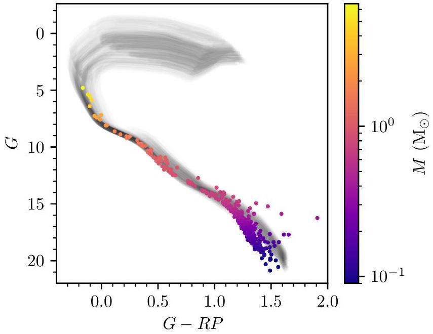
الشكل 1. CMD للنجوم الأعضاء في NGC 2451A مظللة بكتلتها النجمية المحسوبة. تم عرض 100 خط عزل مأخوذ من الورقة الثانية باللون الأسود. (مقتبس من هانت 2023)
للنجوم في ذيول المد والجزر لمجموعة، التي لم تعد مرتبطة بمجموعة الوالد (ماينغاست وآخرون 2021). بافتراض أن المجموعة تملأ سطح روش،من نموذج كينغ (1962) الملائم (بينى وتريمان 1987)، حيث تم استخدام هذه العلاقة في أعمال مثل بيسكونوف وآخرون (2008) لاستنتاج كتل العناقيد المفتوحة بناءً على حجمها.
على الرغم من أن بعض العناقيد المفتوحة، مثل الهيديس، قد أظهرت أن لديها تشتت سرعات نجمية أعلى من المتوقع وهي فوق الحد الحراري وتتفكك، إلا أن هذه العناقيد المتفككة لا تزال كثيفة بما يكفي لتكون ذات جاذبية ذاتية حالياً (أوه وإيفانز 2020، مينغاست وآخرون 2021). وينطبق نفس الشيء على العناقيد الشابة التي تم رصدها مؤخراً في مراحل توسع فوق حرارية محتملة بعد فترة قصيرة من تشكيلها الأولي (كون وآخرون 2019). من ناحية أخرى، فإن المجموعات النجمية من جميع الأنواع (بما في ذلك الجمعيات النادرة من نوع OB) ليست مرتبطة، وتتفكك بنشاط في القرص، مما يعني أنه يجب ألا يكون لديها نصف قطر حيث تمتلك كرة روش، والتي يجب أن تكون قابلة للقياس باستخدام المعادلة 2. في بقية هذا العمل، نهدف إلى تطبيق هذه المعادلة للتمييز بين العناقيد النجمية المرتبطة وغير المرتبطة.
3. حسابات الكتلة ونصف القطر
في هذا القسم، نصف كيف قمنا بحساب الكتل الضوئية وأشعة جاكوب لجميع المجموعات ضمن 15 كيلوبك من الورقة الثانية. تم وصف الكثير من هذه الطريقة في الأصل في هانت (2023)، ولكن تم توضيحها مرة أخرى هنا لتسهيل قراءة هذا العمل. تحتوي هذه الطريقة على خمس خطوات نناقشها في الفقرات الفرعية التالية. أولاً، قمنا باشتقاق الكتل الضوئية للنجوم الأعضاء في كل مجموعة. بعد ذلك، قمنا بتصحيح تأثيرات الاختيار. ثم طبقنا تصحيحًا للنجوم الثنائية غير المحلولة. بعد ذلك، تم ملاءمة دوال الكتلة ودمجها لحساب الكتلة الإجمالية للمجموعة. أخيرًا، تم تكرار هذه العملية عند أشعة مختلفة للعثور على شعاع جاكوب لكل مجموعة.
3.1. حساب الكتل النجمية
اتباعًا لطريقة مشابهة لتلك المستخدمة في أعمال مثل Meingast et al. (2021) و Cordoni et al. (2023)، بدأنا باستخدام ملاءمات الإيزوكرون PARSEC (Bressan et al. 2012) من الورقة الثانية لـ تقدير كتل النجوم الأعضاء في كل تجمع. لحساب كتل النجوم، استخدمنا الكتلة المتوقعة للنجوم كدالة لـ-مقدار النطاق من النماذج التي قمنا بتناسبها في ورقتنا الثانية،“، التي كانت دقيقة لمعظم أعضاء العنقود. ومع ذلك، فإن أقدم العناقيد في عينتنا تحتوي غالبًا على نجوم عملاقة متطورة.-مقدار -باند أقل من قمة التسلسل الرئيسي في العنقود – مما يعني أنليس هناك تطابق واحد لواحد من السطوع إلى الكتلة لبعض أعضاء العنقود. لذلك، في المناطق التي لا تحتوي فيها منحنيات العمر التي قمنا بتناسبها من PARSEC على تطابق واحد لواحد من السطوع إلى الكتلة، استخدمنا أيضًامؤشرات اللون لتحديد أفضل كتلة نجمية لعضو معين في العنقود. قررنا عدم استخدام الـفهرس معظم النجوم كـ و غالبًا ما يتم التقليل من تقدير اللمعان للنجوم الحمراء أو الزرقاء جدًا ذات اللمعان (رييلو وآخرون 2021). المناطق التي نستخدم فيها كانت مؤشرات اللون ليست ضمن النطاقات حيث و تُعتبر مُقللة من قيمتها، ومع ذلك، بسبب اللون الأزرق لهذه المناطق وبسبب وجود العناقيد التي درسناها ضمن 15 كيلوبارسيك.
لدمج عدم اليقين في ملاءمات الإيزوكرون لدينا من الورقة الثانية، قمنا بتكرار هذه العملية 100 مرة لـ 100 إيزوكرون مأخوذ من شبكة الأعصاب الاستدلالية المتغيرة في الورقة الثانية. وقد شمل ذلك عدم اليقين في العمر، والانقراض، والمسافة إلى النجوم في تقديرات الكتلة لدينا لها. توضح الشكل 1 هذه العملية لـ NGC 2451A، حيث تعرض 100 إيزوكرون مأخوذ من الورقة الثانية وكتل النجوم المقدرة لكل نجم مع تظليل النقاط.
من الجدير مناقشة المزيد من القيود والافتراضات لهذه الطريقة. أولاً، نظرًا لأن معلماتنا الضوئية في الورقة الثانية لا تشمل المعدنيات، فإن كتلنا متحيزة للعناقيد ذات المعدنيات المنخفضة أو العالية بشكل خاص. لتحديد هذا النظام، قمنا بتكرار كامل خط أنابيبنا على 143 عنقودًا مختارًا عشوائيًا ولكن مع افتراض معدنياتو -0.5 دكس، اختبار كيفية تغير الكتل المعطاةالقيم عند الحدين الأعلى والأدنى لتلك الملاحظة في الكواكب الخارجية (خارشنكو وآخرون 2013؛ بوسيني وآخرون 2019). بافتراض وجود معدنية عالية، فإن ذلك يزيد الكتل بمعدلبينما يقلل انخفاض المعدنية من الكتل بمعدلالمتوسط المعدني للعناقيد المفتوحة (OCs) يقارب المعدن الشمسي (خارشنكو وآخرون 2013)، لذا فإن هذه القيم هي حدود حالة حافة ستؤثر بشكل رئيسي على العناقيد التي تقع عند أنصاف أقطار مجرية مرتفعة أو منخفضة بشكل خاص والتي من المرجح أن تحتوي على معدنيات غير شمسية (سبينا وآخرون 2022). في المستقبل، سيكون من المهم تضمين تقديرات المعدن الطيفي في استنتاج معلمات العناقيد المفتوحة باستخدام التعلم الآلي لتحسين دقة كتل العناقيد المفتوحة بشكل أكبر.
النقطة التالية التي يجب ملاحظتها هي أن تأثيرات النجوم الثنائية لم تُدرج في نظام الاستيفاء الخاص بنا. وبالتالي، فإن تقديرات كتلة النجوم لدينا هي فقط تقديرات لكتلة النجم الرئيسي في أي نظام ثنائي. للتخفيف من هذا التأثير، قمنا بتطبيق تصحيح على دالة كتلة العنقود الكلية للثنائيات غير المحلولة في القسم 3.3.
أخيرًا، يؤثر استخدامنا لخطوط العمر PARSEC أيضًا على الكتل النجمية المستمدة لدينا، وقد تختلف تقديرات الكتلة لدينا عن تلك المستمدة باستخدام نماذج تطور نجمي أخرى. لقد بحثنا في كيفية تأثير استخدام خطوط العمر MIST (تشوي وآخرون 2016) على تقديرات الكتلة لدينا، من خلال إجراء مقارنات محدودة بين خطوط العمر PARSEC التي قمنا بتناسبها وخطوط العمر MIST في نفس العمر.لـ PARSEC و MIST، فإن الإيزوكرونات عمومًا متشابهة جدًا لـفي جميع الأعمار، ومن ثمللمجموعات عند مسافات أكبر من 1 كيلوبارسيك (حيث أن معظم النجوم المرصودة أكبر من هذه الكتلة) ستكون مشابهة. نحن نقدر أن الكتل الإجمالية المستمدة من MIST ستظل أقل من تلك المستمدة من PARSEC لمثل هذه المجموعات، على الرغم من أنه لا يزيد عنأقل. ومع ذلك،أقل بشكل ملحوظ في MIST مقارنة بـ PARSEC للنجوم ذات الكتل الأقل منفي جميع الأعمار
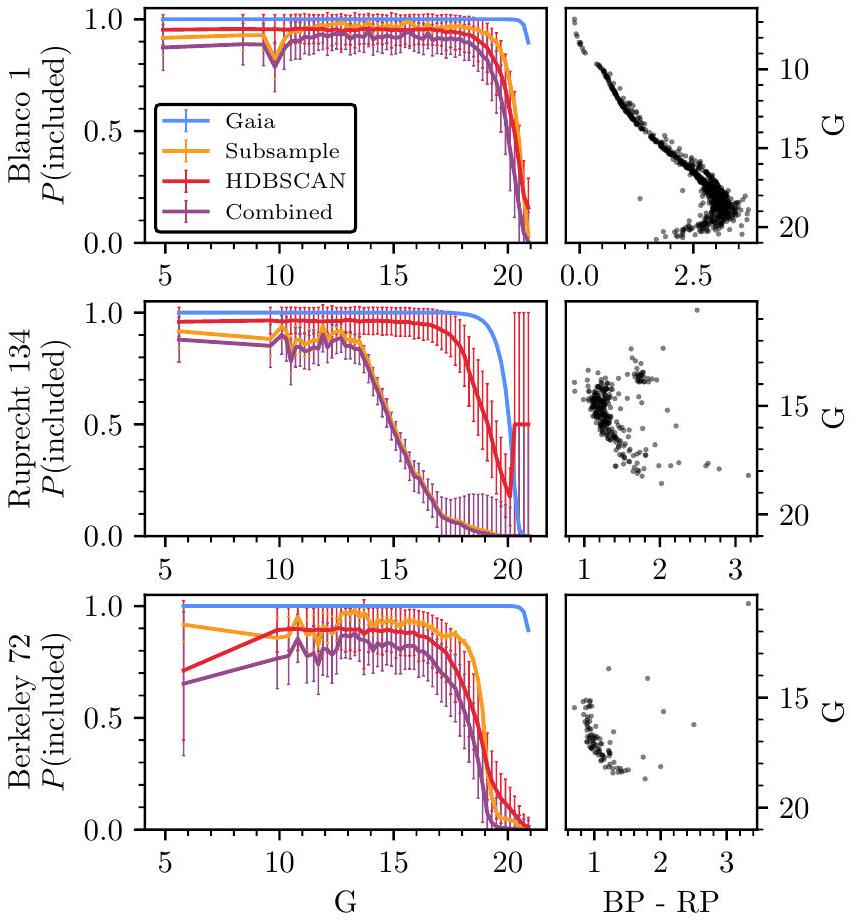
الشكل 2. دوال اختيار الكتل المحسوبة لبلانكو 1 (الصف العلوي)، روبرت 134 (الصف الأوسط)، وبيركلي 72 (الصف السفلي). تُظهر اللوحة اليسرى في كل صف دوال اختيار غايا المعتمدة لدينا (بالأزرق)، العينة الفرعية (بالبرتقالي)، والخوارزمية (HDBSCAN، بالأحمر) كدالة للسطوع لكل كتلة، بالإضافة إلى دالة الاختيار الكلية المضاعفة (بالأرجواني). يتم عرض CMD لكل كتلة كمرجع في اللوحات اليمنى. (مقتبس من هانت 2023)
مما يعني أن النجوم ذات الكتلة المنخفضة ستُعطى كتلًا أقل بواسطة مخططات MIST الإيزوكرونية عند نفس السطوع. نحن نقدر أن هذا سيؤدي إلى كتل إجمالية للعناقيد لا تزيد عنأقل للمجموعات ضمن 300 فرسخ فلكي (التي تتأثر دوال الكتلة فيها بشكل أكبر بالنجوم منخفضة الكتلة حيث يكون هناك أقل توافق بين خطوط العمر MIST وPARSEC).
3.2. تصحيح لتأثيرات الاختيار
على الرغم من أن قوائم عضوية مجموعة ورقتنا الثانية كانت تهدف إلى أن تكون شاملة قدر الإمكان، مع قوائم عضوية تشمل نجومًا خافتة تصل إلىلا تزال هناك عدد من تأثيرات الاختيار التي تحد من اكتمال قوائم عضويتنا والتي يجب أخذها في الاعتبار لاستنتاج كتل المجموعات بدقة. من خلال فحص CMDs للمجموعات التي يصعب استعادتها، مثل تلك الموجودة في مناطق الازدحام العالي حيث تصبح بيانات Gaia غير مكتملة (تعاون Gaia وآخرون 2021) أو المجموعات البعيدة حيث يمكن أن تفوت تقنيتنا المعتمدة في التجميع نجوم الأعضاء (الورقة الثانية)، هناك بوضوح تأثيرات اختيار ستؤثر خلاف ذلك على دوال الكتلة المستنتجة لدينا. في هذا القسم الفرعي، نصف كيف نقوم بنمذجة تأثيرات الاختيار التي تؤثر على كل من قوائم عضوية مجموعاتنا. نشير إلى القراء إلى Hunt (2023) لمزيد من التفاصيل حول طريقتنا.
نعتبر ثلاثة تأثيرات مختلفة قد تؤدي إلى عدم وجود نجم حقيقي في قوائم عضويتنا. أولاً، هناك احتمال أن يكون نجم معين بمعاييريظهر في كتالوج Gaia DR3 الذي يحتوي على 1.8 مليار مصدر،. ثم، هناك الاحتمالية الشرطية بأن يكون مصدر في Gaia DR3 قد تم تضمينه في مجموعة بيانات Gaia التي استخدمناها لتحليل التجميع، وهي جميع النجوم البالغ عددها 729 مليون نجم مع قياسات فلكية كاملة- حل ريك و الضوء، وعلم الفوتومترية، وعلم جودة Rybizki وآخرون (2022) v1 أكبر منفي غايا). أخيرًا، هناك احتمال إضافي أن خوارزمية التجميع المعتمدة لدينا في الورقة الثانية، HDBSCAN (كامبيلو وآخرون 2013، مكينيس وآخرون 2017)، تصنف هذه النجمة كعضو في العنقود،في العينة الفرعية) – والتي تقل احتمالية حدوثها بشكل متزايد اعتمادًا على مدى وضوح فصل مجموعة عن المجال المحيط. هذه التأثيرات مضاعفة (Rix et al. 2021، Castro-Ginard et al. 2023)، مما يعطي احتمالًا إجماليًاأن نجمًا بمعاييريظهر في قائمة عضوية المجموعة المعتمدة لدينا:
المصطلحان الأولان، و في غايا)، يتم حسابها مباشرة من أعمال كانت-غودان وآخرون (2023) وكاسترو-جينارد وآخرون (2023). في العمل الأول، يستنتج كانت-غودان وآخرون (2023) احتمالاً تجريبياً لظهور مصدر في غايا DR3 من خلال مقارنة مجموعة بيانات غايا مع المسوحات الضوئية الأعمق من غايا نفسها. يصفون الاحتمال بأن يكون مصدر ما مدرجًا في غايا بناءً على موقعه، وهو مؤشر جيد على مدى الازدحام في منطقة معينة، بالإضافة إلى…-مقدار النطاق، الذي يعد مؤشراً قوياً على مدى جودة معالجته بواسطة تلسكوب غايا وخط معالجة البيانات. قيم كوظيفة للموقع والحجم تم الاستعلام عنها مباشرة من حزمة بايثون gaiaunlimited (كانت-غودان وآخرون 2023).
بعد ذلك، يوضح كاسترو-جينارد وآخرون (2023) طريقة لتحديد احتمال ظهور مصدر ما في عينة فرعية معينة من مجموعة بيانات غايا.في غايا)، باستخدام طريقة من ريك وآخرون (2021). قمنا بتنفيذ الطريقة التجريبية لكاسترو جينارد وآخرون (2023) كدالة للموقع ومقدار الفرقة وحده، الذي وجدناه مؤشراً جيداً لاحتمالية وجود مصدر في العينة الفرعية المعتمدة لدينا من مجموعة بيانات غايا. كانت العينة الفرعية من بيانات غايا التي استخدمناها في الورقة الثانية تهدف بشكل كبير إلى تقييد تحليلنا ليشمل فقط المصادر ذات الحلول الفلكية عالية الجودة، والتي تتأثر بشدة بالموقع والسطوع. ) لمصدر. نظرًا لأن الطريقة في كاسترو-جينارد وآخرون (2023) تقوم بتجميع المصادر لحساب في غايا)، اخترنا جميع النجوم في المنطقة السماوية التي يغطيها تجمع معين وقمنا بتجميعها حسب-مقدار الباند في صناديق بحجم 0.2 مغ. لمنع نقص العينة في الصناديق للمصادر الساطعة، تم دمج الصناديق حتى تحتوي كل صندوق على عشرة نجوم على الأقل.
أخيرًا، لنمذجة تأثير النقص الناتج عن خوارزمية التجميع التي استخدمناها في الورقة الثانية، قمنا بتطوير تقنية عشوائية لمحاكاة احتمال أن يكون نجمًا حقيقيًا من مجموعة معينة قد تم تعيينه كعضو بواسطة الخوارزمية. تعتمد فرصة تعيين نجم بشكل صحيح كعضو في المجموعة بشكل كبير على دقته الفلكية (الورقة الثانية). بالنسبة لنجم ذو دقة فلكية أقل، ستكون موقعه في الفضاء الخماسي الذي قمنا بالتجميع من أجله أبعد من مركز المجموعة، مما يعني أنه من المرجح أن يتم تفويته بواسطة خوارزمية التجميع لدينا. وهذا ينطبق بشكل خاص على المجموعات البعيدة، حيث تكون عدم اليقين في قياسات غايا غالبًا أكبر من التباين الحقيقي في المنظر أو الحركة المناسبة للمجموعة. نظرًا لأن المجموعات في هذا العمل عمومًا ليست أصغر منفي النطاق الزاوي، فإن الأخطاء الفلكية في موقع النجوم في بيانات غايا الإصدار الثالث (Gaia DR3) تعتبر ضئيلة مقارنةً بحجم العناقيد، لذا فإن هذا التأثير يعتمد فقط على دقة الحركة المناسبة والبارالاكس لأعضاء العنقود.
تم نمذجة هذا التأثير من خلال إجراء محاكاة لما إذا كانت النجوم ذات القياسات الفلكية المحاكية ستظهر داخل تجمع. لكل تجمع، قمنا بمحاكاة 100000 نجم بتوزيع موحد في نطاقتم تعيين أخطاء قياسات الفلك لكل نجم من خلال اختيار نجوم عشوائيًا ذات سطوع مشابه في محيط العنقود الحقيقي واستخدام أخطائها مباشرة. ثم تم إجراء عشرة عينات عشوائية من الحركات المناسبة والبارالاكس لكل نجم. لتقدير ما إذا كان سيتم تصنيف كل نجم محاكى كعضو في عنقود معين أم لا، قمنا بتناسب شكل بيضاوي ثلاثي الأبعاد مع الحركات المناسبة والبارالاكس لأعضاء عنقود ورقتنا الثانية لكل عنقود، ثم حسبنا مدى تكرار ظهور كل نجم محاكى داخل كل شكل بيضاوي مناسب لحساب احتمال أن يكون نجم معين مدرجًا في قائمة عضويتنا.
تظهر وظائف الاختيار المقدرة وCMDs لثلاثة تجمعات نجمية في الشكل 2، موضحة كيف أن تجمعات نجمية مختلفة لها CMDs تهيمن عليها تأثيرات مختلفة. في الحالة الأولى، بلانكو 1 هو تجمع نجمي ذو ارتفاع مجري عالٍ، قريب ( )، سهل الكشف عنه ومنفصل بوضوح عن المجال. لديه CMD مكتظ بصريًا إلى درجات سطوع أضعف حتى من . ينعكس هذا في وظيفة الاختيار المقدرة له، والتي تكون مكتملة إلى حد كبير لـ . من ناحية أخرى، روبرت 134 هو تجمع في مجال مزدحم للغاية بالقرب من مركز المجرة ()، ويعتبر واحدًا من أكثر التجمعات نقصًا في كتالوج ورقتنا الثانية. يتأثر بشدة بتأثير الاختيار من عينة فرعية لدينا، والتي تزيل عددًا كبيرًا من المصادر ذات القياسات الفلكية الشاذة بسبب الازدحام – بالإضافة إلى وظيفة الاختيار لـ Gaia DR3، التي تنخفض بشكل حاد عند في هذه المنطقة. أخيرًا، بيركلي 72 هو تجمع أكثر بعدًا (). نظرًا لبعده وندرة نسبية، فإن وظيفة اختياره تهيمن عليها في الغالب وظيفة الاختيار لخوارزمية التجميع لدينا، على الرغم من أن وظيفة اختيار العينة الفرعية تساهم أيضًا بسبب موقع التجمع في منطقة مزدحمة إلى حد ما من القرص المجري. من هذه الأمثلة الثلاثة فقط، من الواضح أن جميع تأثيرات الاختيار الثلاثة تؤثر على كل تجمع بطرق مختلفة يجب أخذها بعين الاعتبار.
بالإضافة إلى ذلك، من الجدير بالذكر أنه لا يُقدّر أن أي تجمع يكون مكتملًا عند أي درجة سطوع. نقترح أن العديد من هذه النجوم المفقودة المحتملة من المحتمل أن تكون نجومًا متعددة. خلال معالجة Gaia DR3، تم افتراض أن جميع النجوم فردية؛ ومع ذلك، فإن الثنائيات ذات الانحرافات الكبيرة عن القياسات الفلكية المثالية للنجوم الفردية ستعاني من أخطاء أعلى في ملاءمتها الفلكية (ليندغرين وآخرون 2021)، ومن غير المرجح أن تظهر في العينة الفرعية من النجوم ذات القياسات الفلكية الجيدة التي تم بناء كتالوج ورقتنا الثانية منها.
3.3. تصحيح للثنائيات غير المحلولة
كانت الخطوة التالية في طريقتنا تصحيح الثنائيات غير المحلولة. نظرًا لأن كتل النجوم المستنتجة لدينا في القسم 3.2 افترضت أن النجوم فردية، فإن التصحيح الإضافي للثنائيات غير المحلولة مهم لتجنب تحيز كتل التجمع النهائية لدينا إلى قيم منخفضة.
من الناحية المثالية، سيكون من الممكن الكشف مباشرة عن جميع الثنائيات في تجمع معين وقياس نسبة الكتلة لكل نظام ثنائي، باستخدام ذلك كتصحيح لكتلة كل نجم المقدرة. ومع ذلك، فإن مثل هذه القياسات المباشرة ليست ممكنة بناءً على بيانات Gaia DR3 وحدها، وخاصة ليس لجميع 7167 تجمعًا في ورقتنا الثانية. درست بعض الأعمال مؤخرًا نسبة النجوم الثنائية في مجموعة فرعية من التجمعات النجمية الموثوقة، بما في ذلك كوردوني وآخرون (2023) الذين يقيسونها لـ 78 تجمعًا و دونادا وآخرون (2023) الذين يقيسونها لـ 202 تجمع ضمن 1.5 كيلوبارسيك. ومع ذلك، فإن كلا العملين قادران فقط على قياس نسبة الثنائيات لنسب الكتلة ,
نظرًا لصعوبة التمييز بين النجوم الثنائية ذات نسبة الكتلة المنخفضة والنجوم الفردية على التسلسل الرئيسي، خاصة في وجود احمرار تفاضلي. خاصةً منذ أن تم إظهار أن نسبة النجوم الثنائية في الجوار الشمسي قد بلغت ذروتها عند لمعظم النجوم التي تقل عن 2 إلى (مو وآخرون 2017)، مما يعني أن العديد من النجوم من المرجح أن تحتوي على ثنائيات مع أقل من القيم التي يمكن قياسها باستخدام Gaia DR3، نستنتج أن القياسات المباشرة القوية لنسبة الكتلة لمعظم الثنائيات في التجمعات النجمية غير ممكنة، وبدلاً من ذلك استخدمنا تصحيحًا تقريبيًا لكتل النجوم المعتمدة لدينا يأخذ في الاعتبار الثنائيات عند جميع القيم.
استخلصنا تصحيحات لتطبيقها على وظائف كتل التجمع النهائية لدينا باستخدام نسبة التعددية المصححة لتأثير الاختيار، وتكرار النجوم المصاحبة، وتوزيع نسبة الكتلة للنجوم الميدانية من مو وآخرون (2017). تم محاكاة النجوم الثنائية لكل تجمع بناءً على هذه التوزيعات. لمحاكاة ما إذا كان الثنائي محلولًا، وهو ما يحدث كثيرًا للتجمعات القريبة (دونادا وآخرون 2023)، تم استخدام توزيعات الفترة والانحراف من مو وآخرون (2017) لمحاكاة متوسط الفصل بين كل ثنائي محاكى، والذي تمت مقارنته بعد ذلك مع الدقة الزاوية لـ Gaia DR3 (تعاون Gaia وآخرون 2021). اعتمادًا على المسافة إلى تجمع ونطاق الكتلة لكتلة الدالة التي يجب تصحيحها، يزيد هذا التصحيح للنجوم الثنائية من صناديق الكتلة بمقدار إلى ، بينما يضخم أيضًا عدم اليقين المقتبس لدينا على كتل التجمعات بشكل كبير، بسبب الطبيعة التقريبية لهذه الطريقة. نقدر أنه في أسوأ الحالات، يمكن أن تسهم الأخطاء الناتجة عن افتراضنا لوجود مجموعة من النجوم الثنائية الشبيهة بالميدان في إضافات نظامية تصل إلى على كتل التجمع النهائية لدينا. في المستقبل، سيكون من المهم تحسين الطرق لتحديد أي النجوم هي ثنائيات لتحسين دقة كتل التجمعات النجمية أكثر.
3.4. ملاءمات دالة الكتلة
كانت الخطوة النهائية في خط أنابيب قياس كتلة التجمع لدينا هي ملاءمة دالة كتلة لكل تجمع ودمجها لاشتقاق كتلة تجمع إجمالية، بما في ذلك النجوم الضعيفة جدًا التي لا يمكن ملاحظتها. هناك عدد من الأشكال الوظيفية المختلفة لدوال الكتلة التي يمكن اعتمادها (كراوس وآخرون 2020)، مع شكل شائع هو قانون القوة المكسور مع نقطة كسر عند قيمة مثل (كروب 2001). بعض الأعمال، مثل كوردوني وآخرون (2023)، تستخلص كتل التجمعات بينما تقوم بملاءمة دوال الكتلة لقانون القوة المكسور لكل تجمع. ومع ذلك، نظرًا لأن معظم التجمعات في عينتنا أكثر بعدًا من 1 كيلوبارسيك، أو لديها ، فإنها تحتوي على عدد قليل أو لا تحتوي على نجوم تحت نقطة كسر دالة الكتلة النموذجية البالغة ، مما يجعل من المستحيل ملاءمة دوال الكتلة ذات الجزئين لها. إن استقراء دوال الكتلة لقانون القوة المفردة المقاسة للنجوم عالية الكتلة إلى كتل النجوم المنخفضة سيؤدي إلى تقديرات مفرطة لكتل التجمعات لدينا في هذه الحالات، حيث تم قياس أن التجمعات تتشكل بدوال كتلة أقل انحدارًا بشكل ملحوظ عند كتل حوالي وأقل (كراوس وآخرون 2020). بدلاً من ذلك، اعتمدنا نهجًا ‘أكثر أمانًا’، وقمنا بملاءمة فقط دالة كروب (2001) IMF (المشار إليها فيما بعد بـ IMF كروب) لكل تجمع.
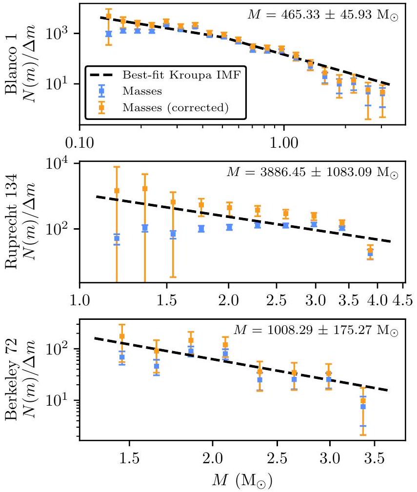
لملاءمة دوال كتل التجمعات، استخدمنا حزمة imf بايثونوأجرينا ملاءمة المربعات الصغرى لسعة كل دالة كتلة تجمع بعد تصحيحها لتأثيرات الاختيار والثنائيات غير المحلولة. بشكل عام، وجدنا أن الغالبية العظمى من التجمعات كانت لديها دوال كتلة تقريبًا بواسطة IMF كروب، على الرغم من أنه فقط بعد تصحيح الكتل لتأثيرات الاختيار والثنائيات. يظهر الشكل 3 دوال الكتلة للتجمعات الثلاثة من الشكل 2، جميعها لها انحدارات تقريبًا بواسطة
الشكل 3. دوال الكتلة للتجمعات الثلاثة من الشكل 2. تُظهر الكتل النجمية الأصلية المجمعة بواسطة المربعات الزرقاء، بينما تُظهر الكتل المجمعة المصححة لتأثيرات الاختيار والثنائيات غير المحلولة بواسطة المربعات البرتقالية. تُظهر الخط الأسود المتقطع IMF كروب الملاءمة لدينا، مع كتلة التجمع الإجمالية المحسوبة لدينا وعدم اليقين المقابل في الزاوية العليا اليمنى. (مقتبس من هانت 2023)
IMFs كروب بعد دمج التصحيحات. يقارن القسم 5.3 دوال كتل التجمعات لدينا بـ IMF كروب بشكل أكبر.
أخيرًا، لتحويل IMF الملاءمة لدينا إلى كتلة تجمع إجمالية، تم دمج كل IMF ملاءمة من حد أدنى قدره إلى أعلى كتلة نجمية تم ملاحظتها في التجمع. هذا الحد الأدنى أقل قليلاً من الحد الأدنى البالغ المستخدم في بعض الأعمال الأخرى (مثل مينغاست وآخرون 2021) والذي يتوافق مع الحد الأدنى للكتلة الذي لا يزال يحدث فيه الاندماج النووي. يشمل حدنا الأدنى البالغ عمدًا أيضًا الأقزام البنية، التي تُلاحظ أيضًا في التجمعات النجمية (موراكس وآخرون 2003) – ولكن يتوقف عن الدمج من ، حيث تعتبر الأجسام المصاحبة حول النجوم ذات الكتل أقل من غالبًا كواكب ولها IMF غير محدد بشكل جيد (أكيزون وآخرون 2013)، وكمية هذه الأجسام التي تطفو بحرية أيضًا غير محددة بشكل جيد. ومع ذلك، فإن اختيار الحد الأدنى يحدث فرقًا ضئيلًا على الكتلة النهائية للتجمع بقدر .
3.5. استنتاج نصف قطر جاكوب
كانت الخطوة الأخيرة من طريقتنا هي حساب كتلة كل تجمع عند جميع الأشعة، والتي تمت مقارنتها بعد ذلك مع نصف القطر الجاكوبى المتوقع نظريًا لتجمع بتلك الكتلة ونصف القطر. وقد نتج عن ذلك احتمال أن يكون لتجمع معين نصف قطر ما حيث يكون فيه الجاذبية أقوى من جاذبية درب التبانة، وبالتالي قياس ما إذا كان تجمع معين يجذب نفسه و(حاليًا) مرتبط.
أولاً، كررنا خط أنابيب قياس الكتلة لدينا عند جميع أشعة التجمع، مستخلصين كتلة التجمع كدالة لنصف قطر التجمع . لم نأخذ في الاعتبار أشعة التجمع حيث كان لدى التجمع أقل من عشرة نجوم أعضاء، حيث يتم تعريف التجمعات المفتوحة عادةً على أنها تحتوي على عشرة نجوم أعضاء على الأقل لتمييزها عن أنظمة النجوم المتعددة (Cantat-Gaudin & Anders 2020، Portegies Zwart et al. 2010). بالإضافة إلى ذلك، قمنا بحساب الكتلة الإجمالية للتجمع بما في ذلك جميع النجوم الأعضاء المعينة (مثل ذيول المد والجزر) .
بعد ذلك، استخدمنا طريقة Meingast et al. (2021) لحساب الكتلة الجاكوبية النظرية كدالة لنصف القطر لكل تجمع، ، من خلال عكس المعادلة 2 يجب افتراض نموذج للجاذبية لحساب و ضمن المعادلة 2. حيث استخدمنا نموذج MWPotential2014 من galpy لجاذبية درب التبانة (Bovy 2015). هذه الجاذبية سلسة، ولا تشمل الأذرع الحلزونية أو السحب الجزيئية العملاقة (GMCs)، ولكن تم ملاءمتها لمجموعة واسعة من البيانات ويجب أن تكون دقيقة بما يكفي لظروفنا. في الممارسة العملية، يعتمد بشكل ضعيف نسبيًا على نموذج الجاذبية المفترض، بسبب اعتماده على الجذر التكعيبي للكمية المحسوبة من الجاذبية. ضمن نموذج الجاذبية المعتمد لدينا، هذه الكمية أكبر فقط بمقدار أربعة أضعاف بين التجمعات عند أدنى الأشعة المجاورة للمجرة في هذه الدراسة ( ) والأعلى ( ). بالإضافة إلى ذلك، نحن مهتمون في هذا العمل بتمييز بين التجمعات المفتوحة والتجمعات المغلقة في الجوار الشمسي، حيث نتوقع أن تكون الجاذبية المجاورة محددة بشكل جيد من قبل هذا النموذج. يمكن أن تكون هذه الترددات بالطبع أقل دقة عند المسافات البعيدة من الشمس، حيث لا تكون الجاذبية المجاورة محددة بشكل جيد.
ومع ذلك، فإن سلاسة نموذج الجاذبية المعتمد لدينا قد تكون مصدرًا للتحيز. نظرًا لكثافتها الغازية المتزايدة مقارنة ببقية المجرة، ستتمتع GMCs والأذرع الحلزونية بجاذبية أقوى، حيث أن الاصطدامات مع GMCs والأذرع الحلزونية تعتبر من المساهمين الرئيسيين في فقدان الكتلة وتدمير التجمعات المفتوحة (Krause et al. 2020). نظرًا للاعتماد الضعيف للمعادلة 2 على نموذج الجاذبية المفترض لدينا، من المحتمل أن يكون هذا التأثير صغيرًا بالنسبة للأذرع الحلزونية، التي تم قياسها لتكون لديها زيادة حوالي في كتلة الغاز (Colombo et al. 2022) – مما يؤدي إلى تغيير صغير فقط في الجاذبية المحلية، حيث ستظل الجاذبية المحلية المؤثرة على تجمع مفتوح في ذراع حلزوني مهيمنة من قبل هالة المادة المظلمة (المفترضة) لدرب التبانة (Bovy 2015، Cautun et al. 2020). ومع ذلك، بسبب كثافتها الغازية الأعلى بشكل ملحوظ، ستكون الجاذبية في GMC نموذجية أعلى بشكل ملحوظ (Krause et al. 2020). نظرًا لأننا مهتمون بشكل خاص بتصنيف المرشحين الجدد المشبوهين للتجمعات المفتوحة في الجوار الشمسي، فمن المحظوظ بعض الشيء أن الشمس تقع داخل فقاعة تحتوي على القليل من الغاز (Zucker et al. 2023). كتحقق إضافي، قمنا بمطابقة كتالوجنا مع كتالوج السحب الجزيئية القريبة في (Cahlon et al. 2024). يوجد تجمع واحد فقط (HSC 598) ضمن 25 فرسخ فلكي من سحابة جزيئية، على بعد 8 فرسخ فلكي. ومع ذلك، تم تصنيف هذا التجمع بالفعل كـ MG بواسطة خط أنابيبنا أدناه، وبالتالي فإن تأثير سحابة الجزيئية المجاورة له على نتائجنا النهائية ضئيل. من المحتمل أن تعمل الأعمال المستقبلية باستخدام مجموعات بيانات أعمق (مثل Gaia DR4 أو DR5) مع كتالوج أعمق يتضمن المزيد من التجمعات حتى مسافات أكبر، وبالتالي قد يتعين أخذ تأثير GMCs والأذرع الحلزونية على الجاذبية المحلية المحيطة بالتجمعات في الاعتبار.
أخيرًا، مع القيم النظرية لـ المحسوبة لكل تجمع، و تمت مقارنتها لتحديد نصف القطر الجاكوبى المحتمل لكل تجمع. إذا كان لدى تجمع ما نصف قطر حيث تكون الكتلة المحصورة ضمن هذا نصف القطر ، فإن يؤخذ كنصف القطر الجاكوبى للتجمع ، مع الكتلة المحصورة المقابلة . في الحالات التي يكون فيها عند جميع الأشعة، يعتبر التجمع أنه ليس لديه نصف قطر جاكوبى صالح وهو MG. بالإضافة إلى ذلك، تحتوي بعض التجمعات على عند جميع الأشعة، مما يعني أن التجمع المرصود أصغر من
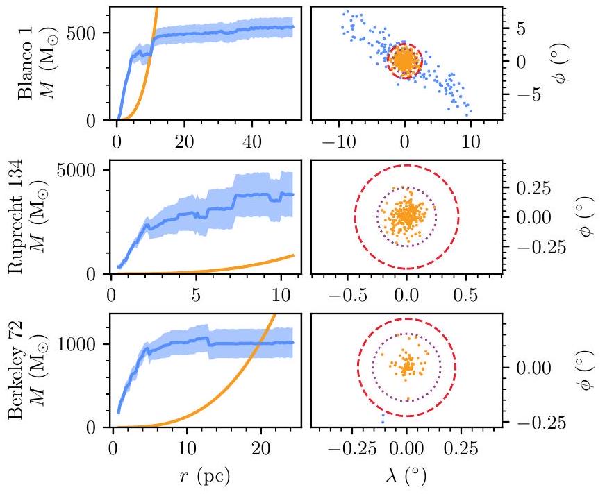
الشكل 4. طريقة حساب نصف القطر الجاكوبى موضحة للتجمعات الثلاثة من الشكل 2. مع كل صف يتوافق مع كل تجمع مفتوح. ضمن كل صف، تُظهر اللوحة اليسرى كتلة التجمع كدالة لنصف القطر من مركز التجمع، حيث الخط الأزرق هو كتلة التجمع الإجمالية المحسوبة لدينا مع منطقة عدم اليقين المظللة، والخط البرتقالي هو الكتلة الجاكوبية النظرية لتجمع بهذا الحجم وفقًا للمعادلة 2. تقاطع هذه الخطوط هو للتجمع. تُظهر اللوحة اليمنى في كل صف التجمع في إطار إحداثي عشوائي مركزي على مركز التجمع. تُظهر النجوم الأعضاء ضمن باللون البرتقالي، مع النجوم الأعضاء خارج باللون الأزرق. يتم الإشارة إليه بواسطة الخط الأحمر المتقطع. الخط البنفسجي المنقط يدل على نصف القطر المداري التقريبي المحسوب لدينا (King 1962) لكل تجمع من الورقة الثانية. (معدل من Hunt 2023)
نصف القطر الجاكوبى للتجمع بناءً على كتلته المرصودة. هذه هي الحالة لبعض التجمعات البعيدة أو الصعبة الكشف، حيث من المحتمل أننا نلاحظ فقط الأجزاء الداخلية من التجمع، ولا نكتشف النجوم حتى نصف القطر الحقيقي للتجمع . في هذه الحالات، استخدمنا النظرية لجميع النجوم المرصودة في التجمع كنصف القطر للتجمع، على الرغم من أن هذه القيم ربما تقلل من تقدير نصف القطر الحقيقي للتجمع . و موضحتان في الشكل 4 لتجمعات بلانكو 1، روبرت 134، وبركلي 72. كما كان متوقعًا لهذه التجمعات الموثوقة، فإن جميعها لديها بوضوح أشعة تكون فيها كتلها المحصورة أعلى من الكتلة الجاكوبية النظرية، مما يعني أنها تجمعات مرتبطة ذات جاذبية ذاتية. كما تم مناقشته سابقًا، يعتبر روبرت 134 تجمعًا صعب الكشف، حيث نجد عند جميع الأشعة، مما يعني أن النجوم الأعضاء الإضافية في أطراف هذا التجمع لم يتم اكتشافها بعد.
ومع ذلك، نظرًا لأننا مهتمون باستخدام أنصاف الأقطار الجاكوبية لتمييز بين التجمعات المرتبطة وغير المرتبطة، فإن أداء هذه الطريقة على التجمعات المشبوهة هو الأكثر صلة. في القسم قبل الأخير من الورقة الثانية، أبرزنا ثلاثة أمثلة على المرشحين الجدد للتجمعات المفتوحة – اثنان منهما بدوا مشبوهين بشكل خاص بسبب توزيعاتهم على السماء التي لا تظهر نواة تجمع ‘كتلية’ واضحة كما هو متوقع لتجمع مفتوح (King 1966). الشكل 5 يُظهر الكتلة كدالة لنصف القطر لهذه التجمعات الثلاثة. التجمعان اللذان أبرزناهما على أنهما لا يشبهان التجمعات المفتوحة، HSC 1131 وHSC 2376، لديهما عند جميع الأشعة، مما يشير بقوة إلى أنهما في الواقع تجمعات غير مرتبطة. من ناحية أخرى، HSC 1186، وهو تجمع لديه كتلة مركزية صغيرة، يبدو متوافقًا مع كونه تجمعًا صغيرًا مرتبطًا بكتلة مرتبطة قدرها ، كما كان متوقعًا أيضًا في الورقة الثانية.
في المجموع، استغرق الأمر أقل من من إجمالي وقت وحدة المعالجة المركزية لإجراء حسابات الكتلة ونصف القطر كما هو الحال مع التجمع الأصلي-
الشكل 5. نفس الشكل 4 ولكن لثلاثة مرشحين جدد للتجمعات المفتوحة من الورقة الثانية: HSC 1131 (الصف العلوي)، HSC 2376 (الصف الأوسط)، وHSC 1185 (الصف السفلي). على الرغم من أن HSC 1131 وHSC 2376 لا يبدو أنهما لديهما نصف قطر جاكوبى، إلا أن نصف القطر الجاكوبى الأكثر احتمالًا لهما لا يزال موضحًا في الرسوم البيانية في العمود الأيمن. (معدل من Hunt 2023)
الشكل 6. توزيع لجميع التجمعات في هذا العمل، وهو احتمال أن يكون للتجمع نصف قطر جاكوبى صالح. (معدل من Hunt 2023)
تحليل الورقة الثانية استغرق. لا يبدو أن هذه الطريقة قابلة للتطبيق لتمييز بين التجمعات المفتوحة والتجمعات المغلقة فحسب، بل إنها أيضًا ليست تحديًا حسابيًا خاصًا، مما يعني أنه يمكن دمجها بشكل معقول في أي بحث مستقبلي عن التجمعات.
4. النتائج
قمنا باشتقاق أنصاف أقطار جاكوبى والكتل لـ 6956 تجمعًا ليست تجمعات كروية وتقع على بعد أقل من 15 كيلوبكسل. نظرًا لأن التجمعات التي تبعد أكثر من 15 كيلوبكسل لم تُدرج في بيانات التدريب لشبكة الأعصاب في ورقتنا الثانية، كانت تقديرات أعمارها وانقراضها غير موثوقة للغاية للاستخدام. تم إجراء محاولة لتناسب الإيزوكرونات مع فوتومترية التجمع باستخدام طرق أخرى، على الرغم من أن معظم هذه التجمعات البعيدة كانت ذات جودة منخفضة في مخططات CMD، مما جعل من المستحيل اشتقاق تقديرات دقيقة لبارامترات هذه التجمعات باستخدام بيانات غايا فقط. يجب التحقيق في هذه التجمعات البعيدة بشكل منفصل في عمل آخر، خاصةً منذ أن تم استخدام نموذجنا المعتمد لإمكانات درب التبانة لحساب
الجدول 1. كتالوج تجمعات النجوم مع الكتل، تصنيفات الأجسام، وأشعة جاكوب.
اسم
نوع
بلانكو 1
0
710
841
1.00
2.97
10.65
465.33 (45.93)
٥٢٩.٠٩ (٥٧.٦٧)
HSC 1142
م
–
159
0.00
–
–
–
١٠٩.٧٣ (٢٠.٠٢)
HSC 180
م
–
٢٤
0.00
–
–
–
٢٤.٨٣ (٥.٣٥)
إتش إس سي 2068
م
–
٢٨
0.01
–
–
–
14.87 (4.32)
HSC 2327
م
١٣
91
0.99
1.83
3.04
10.75 (3.79)
64.43 (13.20)
HSC 242
م
–
62
0.00
–
–
–
٣٦.٦٥ (٦.٤٥)
HSC 2603
م
–
26
0.00
–
–
–
17.67 (4.35)
HSC 2907
أو
229
٣٤٩
1.00
3.07
6.96
132.83 (13.41)
184.66 (22.60)
HSC 719
م
–
٢٩
0.00
–
–
–
16.69 (2.32)
HSC 782
م
٢٢
٤٧
1.00
0.84
٣.٣٠
١٣.٦٦ (٣.٢٨)
٢٥.٩٠ (٦.٩٩)
IC 2391
أو
316
٣٧٦
1.00
1.98
7.66
١٦٩٫٤٣ (٢٥٫٣٩)
203.89 (27.55)
IC 2602
أو
٤٤٠
٦٣٨
1.00
٣.٤٦
8.52
٢٣٧٫٢٥ (٣٢٫٤٥)
344.16 (42.26)
ماماجيك 2
0
٩٨
226
1.00
3.10
6.10
90.56 (4.21)
205.71 (14.24)
ميلوت 20
0
738
938
1.00
٤.٢٨
10.30
٣٩١.٦٢ (٥٤.١١)
٥٠٢.٨٠ (٦٥.٩١)
ميلوت 22
أو
١٦٣٩
1721
1.00
3.61
13.69
946.51 (86.77)
984.55 (92.36)
ميلوت 25
0
569
927
1.00
٤.٠٨
8.06
193.04 (42.64)
٤٠٩.٠٠ (٥٦.٩٥)
إن جي سي 2632
أو
١٢٢٤
1314
1.00
3.95
13.73
945.01 (72.73)
١٠١٢.٠١ (٧٣.٧١)
OCSN 49
م
–
٢٦٥
0.31
–
–
–
218.82 (23.91)
بلاتيس 10
أو
٥٨
١٩٧
1.00
٢.٥٠
٤.٧٤
42.94 (8.73)
١٦٦٫٧٩ (١٩٫٧٧)
UPK 612
م
٢٨
228
1.00
1.57
٣.٢٠
٢٨.٦٠ (٦.٢٨)
١١٢.٧٩ (٢٨.٦١)
ملاحظات. موضحة لاختيار عشوائي من عشرة كائنات أصلية وعشرة كائنات مجمعة في العينة عالية الجودة ضمن 250 فرسخ. الأخطاء في الكتل موجودة بين الأقواس. الجدول الكامل متاح في المواد عبر الإنترنت، ويشمل جميع المعلمات المستمدة في الورقة الثانية. وقد تكون أقل دقة عند المسافات التي تزيد عن 15 كيلوبارسيك. في القسم التالي، نقدم هذه النتائج العامة ونقارن كتل المجموعات لدينا مع القيم الموجودة في الأدبيات.
4.1. تعريفات محدثة للتجمعات من الورقة الثانية
بفضل طريقة استنتاج نصف قطر جاكوبى، نحن الآن قادرون على تقديم تعريفات محدثة للتجمعات في كتالوج ورقتنا الثانية. في القسم التالي، نناقش كيف تؤثر إضافة هذه الطريقة على كتالوجنا.
قمنا بحساب احتمال أن يكون للعنقود نصف قطر جاكوبي صالح.، حيث يتم عرض التوزيع في الشكل 6.827، فإن العناقيد غير متوافقة بشدة مع وجود مكون مقيد، مع. من ناحية أخرى، حوالي 5733 مجموعة تتوافق بشكل قوي مع وجود نصف قطر جاكوبى صالح، مع 397 تجمعًا تحتوي على قيم بين هذين الحدين. تبدو الكتل وأشعة جاكوبى طريقة ناجحة للتفريق بين الأجسام المرتبطة وغير المرتبطة. على عكس المحاولات السابقة لاستخدام نظرية الفيريل للتمييز بين العناقيد المفتوحة والمجموعات النجمية أثناء إعداد هذا العمل (انظر القسم 2)، فإن احتمال أن يكون لتجمع معين شعاع جاكوبى صالح هو أكثر نجاحًا في التمييز بين التجمعات المرتبطة وغير المرتبطة.
ومع ذلك، لا يزال يبدو أن طريقتنا الحالية تعاني من قيود في نهاية الكتلة المنخفضة. بعض المجموعات النجمية من الورقة الثانية، مثل المنطقة الأكثر كثافة منتُقاس كتلة جاكوبى الصغيرة لمجموعة توكاناى MG – عادة أقل من، ولكن غالبًا ما يكون أقل من. بينما يشير هذا إلى أن هذه المجموعات تحتوي على مناطق مرتبطة منخفضة الكتلة مضغوطة تقع في مكان ما بين تعريفات نظام النجوم المتعددة أو تجمع النجوم، هناك أيضًا عدة أسباب تجعل هذه الأشعة جاكوبى المنخفضة قد تكون أخطاء. أولاً، من خلال افتراض دالة الكتلة الأولية لكروب، ستكون تقديراتنا للكتلة متحيزة نحو قيم أعلى محافظة للمجموعات النجمية المتطورة ديناميكيًا التي فقدت نجومًا منخفضة الكتلة على مدى فترة طويلة من التفاعلات الثنائية. في هذه الحالات، ستظهر مجموعة كثيفة من اثني عشر نجمًا عالي الكتلة كتلة إجمالية مبالغ فيها باستخدام طريقتنا، وهو ما سيكون صحيحًا بشكل خاص للمجموعات النجمية التي تعاني من تمييز الكتلة. ثانيًا، هناك افتراض ضمني في استخدامنا للمعادلة 2 وهو أن مجموعة النجوم متجانسة كرويًا (بينى وتريمان 1987). قد ينهار هذا الافتراض لمجموعات صغيرة من اثني عشر نجمًا في أكثر المناطق كثافة في مجموعة النجوم. بعض الأمثلة على المكونات منخفضة الكتلة من المجموعات النجمية التي يبدو أنها تمتلك نصف قطر جاكوبى صالح تنتهك بوضوح هذا الافتراض، وبالتالي قد يتم قياسها بشكل خاطئ على أنها تمتلك نصف قطر جاكوبى صالح.
وبالتالي، نوصي أيضًا باستخدام حد أدنى إضافيمنعند اتخاذ القرار بين حبوب منع الحمل والأجهزة داخل الرحم. هذا الحد الأدنى أعلى من حتى أصغر الكتل المعترف بها على نطاق واسع، مثل ميلوت 111 (كومه بير) أو بلاتيس 9، ولكنها تستثني الحالات الحدودية التي تبدو كأنها مناطق كثيفة من MGs حيث تتعطل طريقتنا، أو الحالات التي قد تكون أفضل تصنيفًا كنظام نجمي متعدد مُحلل. الكتل التي تقل عن حد الكتلة هذا والتي لديها قيمة عالية مقاسة منستظل كائنات مثيرة للاهتمام لدراسة متابعة حول سبب ظهور بعض المجرات القزمة بقلوب كثيفة. يمكن أن تكون هذه القلوب الكثيفة، على سبيل المثال، بقايا لكتلة مفتوحة تم حلها.
في المجموع، يحتوي كتالوج ورقتنا الثانية على 5647 عنقودًا ) مع كتلة دنيا من، وعشر نجوم مرصودة على الأقل ضمنفي الجوار الشمسي، يتم تصنيف معظم المجموعات من الورقة الثانية على أنها MGs، مع (26 من 234) تجمعات ضمن 250 فرسخ فلكي تتوافق مع تعريفنا للكتل المفتوحة. ضمن 100 فرسخ فلكي، هناك فقط كتلتي OCs: ميلوت 25 (الهيدس) وميلوت 111 (كومه بير). من بين التجمعات الجديدة المبلغ عنها في الورقة الثانية، 1441 من 2387 تتوافق مع كونها كتل مفتوحة، أو 487 من 739 تجمعًا جديدًا عالي الجودة من الورقة الثانية. هذا يتماشى مع اعتقادنا في الورقة الثانية بأن نسبة كبيرة من التجمعات الجديدة المبلغ عنها لم تبدُ ككتل مفتوحة. من المدهش أن سبعة تجمعات جديدة تم الإبلاغ عنها في الورقة الثانية ضمن 250 فرسخ فلكي تتوافق.
الجدول 2. نجوم الأعضاء في المجموعات المفتوحة والمجموعات الكروية ضمن 15 كيلوبارسيك بكتل نجمية فردية.
اسم
معرّف المصدر
في
القداس )
بلانكو 1
٢٣٨٠٥٧١٩٣٥٤٧١٣٣٠٥٦٠
0
بلانكو 1
2320987858469300864
1
بلانكو 1
2320786540467288320
1
بلانكو 1
٢٣٣٢٩٠٨٧٢٩١٧٨٢٥٨٥٦٠
1
بلانكو 1
2320757850084772480
1
بلانكو 1
2320550046683235328
1
بلانكو 1
2332928451667849856
1
بلانكو 1
2314778985026776320
1
بلانكو 1
2334068503491984896
0
بلانكو 1
2330660983812933376
0
ملاحظات. موضحة لعشرة نجوم أعضاء من بلانكو 1. الجدول الكامل متاح في المواد عبر الإنترنت، ويشمل جميع المعلمات المدرجة في جدول النجوم الأعضاء في الورقة الثانية من بيانات غايا DR3.
الجدول 3. إجمالي عدد أنواع المجموعات.
نوع
ملصق
معايير
عد
(عالي الجودة)
OC
أو
و
5647
٣٥٣٠
إم جي
م
أو
1309
539
– لا
992
٣٠١
– لديه
317
238
جي سي
ج
التطابق المتقاطع
132
٢٥
بعيد جداً
د
62
٦
مرفوض
ر
دليل
17
–
ملاحظات.عدد الكتل من نوع معين الموجودة أيضًا في العينة عالية الجودة من الكتل من الورقة الثانية، وهي تلك التي لديها فئة CMD متوسطة أكبر من 0.5 ونسبة إشارة إلى ضوضاء فلكية (CST) أكبر منالعناقيد المعرفة كعناقيد كروية في فاسيلييف وباومغارت (2021)، خارشينكو وآخرون (2013)، أو غران وآخرون (2022).تمت مطابقة الكتل لاحقًا مع المجرات أو المجرات القزمة، أو تمت إزالتها بسبب كونها أخطاء واضحة في خوارزمية التجميع (انظر القسم 4.1). مع كونها كائنات أصلية، على الرغم من أن جميعها باستثناء واحدة لها كتل منخفضة منأو أقل.
تم تقديم نسخة محدثة من كتالوج الورقة الثانية تشمل تصنيفات الأجسام والكتل في الجدول 1. بالإضافة إلى ذلك، تم تقديم نسخة محدثة من قوائم العضوية النجمية للورقة الثانية لكل تجمع (بما في ذلك الكتل النجمية الفردية) في الجدول 2. يوضح الجدول 3 الإحصائيات العامة حول العدد الإجمالي للتجمعات حسب نوع الجسم والعينة.
بالإضافة إلى ذلك، تم دمج بعض التحديثات على الأسماء في الكتالوج. أولاً، تم تحديث أحد عشر تجمعًا إضافيًا ليتم تصنيفها كعناقيد كروية: أولاً، HSC 134 وHSC 2890، اللذان هما في الواقع Gran 3 وGran 4 وقد تم الإبلاغ عنهما بالفعل في Gran et al. (2022). بالإضافة إلى ذلك، تم تحديث Palomar 2 و6 و8 و10 و11 و12، وIC 1276، و1636-283 (الذي تم تغيير اسمه إلى ESO 452-11 الأكثر استخدامًا)، وPismis 26 ليتم تصنيفها كعناقيد كروية كما في Kharchenko et al. (2013) وPerren et al. (2023).
بعد ذلك، تم تمييز 17 مجموعة تتوافق بوضوح مع المجرات أو المجرات القزمة، أو الأخطاء في خوارزمية التجميع لدينا في الكتالوج (النوع ). تم تسليط الضوء على هذه المجموعات من قبل أعضاء المجتمع في الأشهر التي تلت نشر حسب II (غروشفيدل، اتصال خاص؛ أليسي، اتصال خاص- الاتصالات)، ويجب عدم استخدامها في دراسات تجمعات النجوم المجرية.
أخيرًا، قمنا بإدراج عدد من تصحيحات الأسماء من بيرين وآخرون (2023)، وتويتش (تواصل خاص)، ورورسر وشيلباخ (تواصل خاص). هذه التصحيحات مدرجة في الجدول A.1 وتشمل تصحيحات للأخطاء المطبعية، وتغييرات في بعض الأسماء لتكون متسقة مع مجموعات أخرى تحمل نفس التسمية، وتغييرات في المجموعات من ليو وبانغ (2019) لتكون التسمية الأكثر شيوعًا ‘LP’ بدلاً من ‘FoF’، وإدراج ورقة تم تفويتها من المطابقة المتقاطعة في الورقة II ومن قبل كتالوجات OC الأخرى (كرونبرغر وآخرون 2006). تحتفظ المجموعات بنفس رقم الهوية بين هذا العمل والورقة II، والأسماء السابقة من الورقة II مدرجة في الكتالوج الكامل على الإنترنت.
4.2. التوزيعات العامة للفهرس
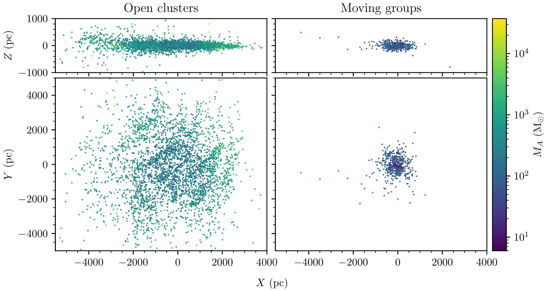
في هذا القسم الفرعي، نقارن الفروق بين التوزيعات المكانية والمعاملات لـ OCs و MGs. توضح الشكل 7 التوزيع في الإحداثيات الكارتيزية الشمسية لعينة عالية الجودة من OCs و MGs. في الورقة الثانية، أشرنا إلى أن كتالوجنا كان لديه قمة غير طبيعية في الكثافة بالقرب من الشمس، مع وجود مئات من العناقيد الإضافية مقارنة بكتالوجات مثل كتالوج كانت-غودين وأندرس (2020)، والتي اقترحنا أنها MGs. يؤكد الشكل 7 هذه الفرضية، حيث يظهر أن الأجسام التي تم تصنيفها الآن على أنها MGs كانت مسؤولة عن قمة الكثافة بالقرب من الشمس، حيث أن MGs جميعها تقع على مسافات أقل بكثير. كما تم الاشتباه به في الورقة الثانية، تهيمن MGs على توزيع العناقيد في الكتالوج بالقرب من الشمس.
توزيعات الكتل للأجسام المفتوحة (OCs) والمجموعات النجمية (MGs) في هذا العمل لها توزيعات مختلفة للمعلمات، مع وجود فرق قوي بشكل خاص في كتلها. تُظهر توزيعات كتل الأجسام المفتوحة والمجموعات النجمية في الشكل 8 أن المجموعات النجمية في هذا العمل أقل كتلة بشكل عام، مع كتلة إجمالية نموذجية تساوي. عادةً ما تكون الكائنات الأصلية (OCs) أثقل بكثير، بكتلة نموذجية تبلغ حوالي.
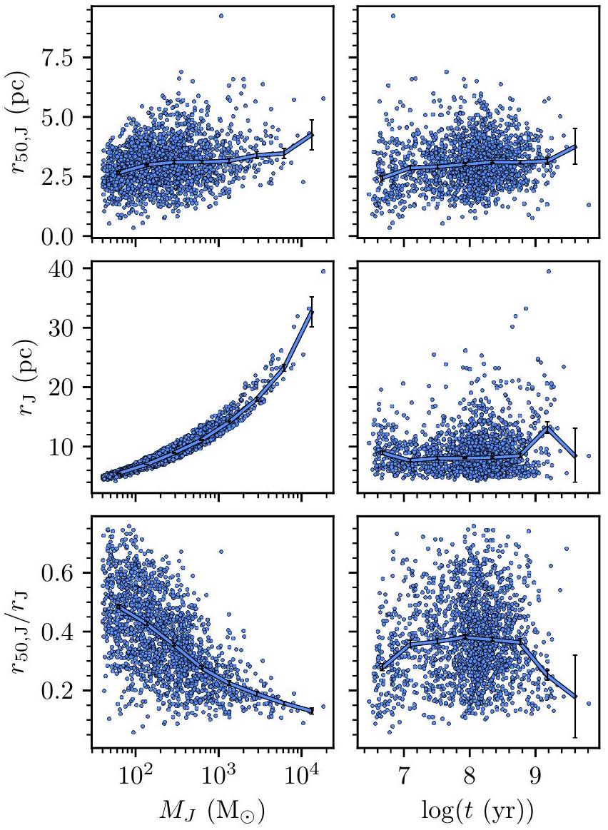
تظهر أشعة OC و MG أيضًا عددًا من الاختلافات والارتباطات المثيرة للاهتمام التي يمكن مقارنتها بالتنبؤات النظرية. توضح الشكل 9 أشعة OC وتركيزاتها مقابل الكتلة والعمر: أي، الشعاع الذي يحتوي علىمن الأعضاء داخلنفسه، ونسبة بين هذين الشعاعين (المماثلة لتركيز العنقود). يتم عرض هذه فقط للأجسام الأصلية في العينة عالية الجودة من الأجسام التي تقع ضمن 2 كيلو فرسخ؛ أي تلك التي تم قياس نصف أقطارها وكتلها وأعمارها بشكل موثوق. كدالة للكتلة، مرتبط بشكل طفيف، حيث أن الكتل ذات الكتلة الأكبر عادة ما تحتوي على نوى أكبر قليلاً.مرتبط ارتباطًا وثيقًا بالكتلة على الرغم من أن هذا متوقع، حيثيتم حسابه مباشرة من كتلة العنقود باستخدام المعادلة 2. كما أن تركيزات العنقود مرتبطة بقوة بكتلة العنقود، حيث أن العنقود الأقل كتلة هو الأقل تركيزًا في المركز، مما يشير بقوة إلى أن العناقيد المفتوحة أقل تركيزًا في المركز كدالة للكتلة، على الأرجح بسبب العمليات الديناميكية داخلها (Portegies Zwart et al. 2010، Krause et al. 2020). ومع ذلك، كدالة للعمر، فإن أشعة وتركيزات العنقود عمومًا غير مرتبطة، على الرغم من أن العناقيد الأصغر سنًا (قد تكون أصغر قليلاً وأكثر تركيزًا، وهو ما يتماشى مع النظرية الحالية التي تفيد بأن الأجسام الكونية تمر بمرحلة من التوسع (Krause et al. 2020). نظرًا لأن الحد الأدنى من العمر الذي يمكن أن يقيسه الشبكة العصبية من الورقة الثانية هوقد لا تكون أعمار العناقيد الشابة مقاسة بشكل كافٍ لتمثيل هذه النطاق من تشكيل العناقيد بشكل مناسب.
على الرغم من أن منهجيتنا لم تكن مخصصة في الأصل لاكتشاف المجموعات النجمية (الورقة الأولى)، إلا أن المجموعات النجمية في كتالوجنا لا تزال نقطة مقارنة مثيرة للاهتمام ضد المجموعات النجمية التي اكتشفناها. الشكل 10 يظهر متوسط أنصاف أقطار المجموعات.إجمالي الأشعة بما في ذلك جميع الأعضاء
الشكل 7. مقارنة التوزيع المكاني للكتل المفتوحة والمجموعات النجمية. العمود الأيسر: التوزيع في إحداثيات هليوسنتريك الكارتيزية لـ 3530 كتلة مفتوحة في العينة عالية الجودة من الكتل المفتوحة من الجدول 3. الشمس في الكمبيوتر، المركز المجري على اليمين، و المحور يدل على الارتفاع فوق أو تحت المستوى. يتم تظليل OCs بواسطة كتلة العنقود المكتشف بالكامل، بما في ذلك الذيل المدّي. العمود الأيمن: رسم بياني مماثل، ولكن لـ 539 MGs في العينة عالية الجودة.
الشكل 8. هيستوغرام الكتل الكلية للمجموعاتلكل المجموعات مقسمة إلى عينات مختلفة. يتم عرض ذلك لجميع المجموعات (خط منقط أسود)، تلك التي مع (خط متقطع أزرق)، وأولئك الذين لديهم (خط متقطع برتقالي). تُظهر النسخ المتقطعة والصلبة من هذه الخطوط توزيع الكتلة لهذه المجموعات ولكن مقصورة فقط على تلك الموجودة في عينة الأجسام عالية الجودة. (مقتبس من هانت 2023)
النجوم وأي ذيول مديةنسبة نصف قطر العنقود الوسيط إلى نصف القطر الكليلـ OCs و MGs عالية الجودة في عينتنا ضمن 2 كيلوبارسيك. حجم MGs المكتشفة يرتبط بقوة بكتلتها – على الرغم من أن هذا قد يكون تأثير اختيار، حيث قد يكون من الأسهل اكتشاف نجوم الأعضاء في MGs على مسافات أكبر إذا كانت أيضًا ذات كتلة أعلى. من الواضح أن MGs تشغل منطقة مختلفة من معلمة نصف القطر-الكتلة. الفضاء بين النجوم، عمومًا يكون أكبر بكثير من العناقيد المفتوحة عند كتلة معينة. لا يبدو أن تركيز المجرات يتغير كدالة للكتلة، وهو ما يختلف عن العناقيد المفتوحة التي يقود تطورها الهيكلي دينامياتها الداخلية (المقيدة) والانحلال التدريجي بسبب جاذبية درب التبانة (كراوس وآخرون 2020).
تختلف MGs و OCs بشكل كبير حسب العمر. تمتلك OCs و MGs أحجامًا مشابهة في الأعمار الصغيرة لـ، مما يشير إلى أصل مشابه. ومع ذلك، بينما تخضع OCs لمرحلة صغيرة من التوسع، فإن MGs تتوسع بشكل أقوى بكثير، مما يجعلها في النهاية أكبر بكثير من OCs في جميع الأعمار الأكبر (خصوصًا لـ.) هذه الزيادة في الحجم الملحوظ تتماشى مع المجموعات النجمية في كتالوجنا التي تعتبر مجموعات غير مرتبطة من النجوم المعاصرة التي تتوسع مع مرور الوقت. ومع ذلك، فإن العديد من المجموعات النجمية المعاصرة أقدم من الوقت المتوقع الذي سيستغرقه تشتتها (زوكير وآخرون 2022). إذا كانت هذه المجموعات النجمية المعاصرة هي مجموعات حقيقية من النجوم المتطورة معًا، فقد تكون بقايا غير مرتبطة من العناقيد النجمية المرتبطة. يجب التحقيق في هذه الأجسام (وتطورها الديناميكي، مثل ما إذا كانت نجومها الأعضاء تتوسع من أصل مشترك أم لا) بشكل أعمق في عمل مستقبلي.
4.3. مقارنة الكتل مع نتائج الأدبيات
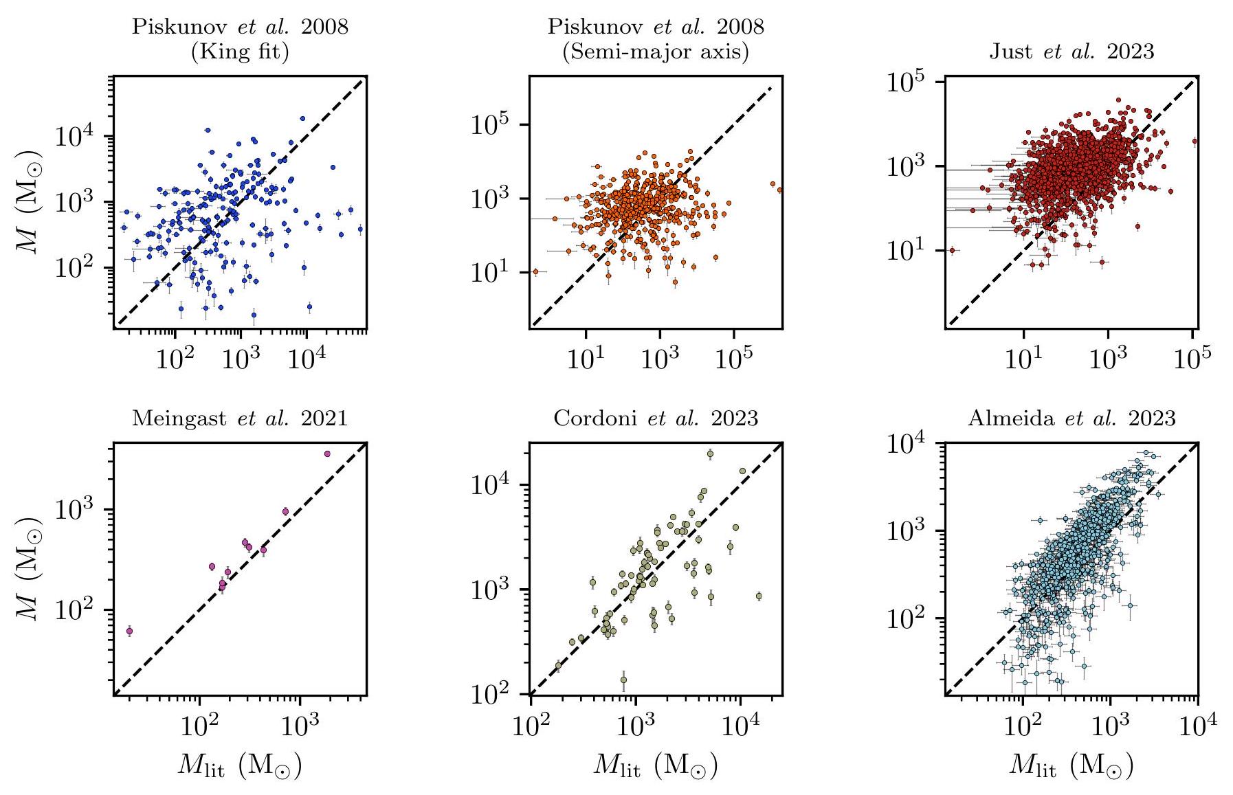
أخيرًا، خطوة مهمة في التحقق من نتائجنا هي مقارنة كتل المجموعات المستمدة لدينا مع النتائج من الأدبيات، على الرغم من أن كتل المجموعات عمومًا لا تقاس بشكل متكرر في الأدبيات وأن المنهجيات المختلفة يمكن أن تنتج نتائج مختلفة تمامًا. يتم مقارنة كتل المجموعات من الأدبيات مع الكتل المستمدة في هذا العمل في الشكل 11. نقارن كتلنا مع الكتل المستمدة بدون بيانات غايا واستخدام تقنيات ملاءمة الملف الشخصي في بيزكونوف وآخرون (2008) وجوست وآخرون (2023)؛ باستخدام فوتومترية غايا DR2 في مينغاست وآخرون (2021)؛ و-
الشكل 9. أنصاف أقطار جاكوبى وتركيزات الكواكب الصغيرة عالية الجودة ضمن 2 كيلوبارسيك، موضحة لـ (الصف العلوي)، (الصف الأوسط)، وتركيزات الكتل (الصف السفلي) مقابل كتلة مجموعة جاكوبى (العمود الأيسر) وعمر المجموعة (العمود الأيمن). في كل لوحة، يتم عرض خط الاتجاه للوسائط المجمعة باللون الأزرق، مع أشرطة الخطأ التي تظهر الخطأ القياسي.
قياس الضوء في Gaia DR3 في كوردوني وآخرون (2023) وألميدا وآخرون (2023).
نجد أن كتلنا تشبه إلى حد كبير العينة الصغيرة المكونة من عشرة تجمعات قريبة التي تم دراستها في Meingast et al. (2021)، الذين طبقوا منهجية مشابهة من خلال افتراض دالة الكتلة لكروب وملاءمتها لدالة الكتلة لتجمع. تقديرات كتلنا أعلى من تقديراتهم، مع كون هذا الاختلاف أكبر بالنسبة لبلاتيس.عنقود يقدره مينغاست وآخرون (2021) أن له كتلة تبلغ فقط، مقارنةً بقياسنا لـفي الواقع، تقديراتنا للكتلة عمومًا أعلى من تقديرات جميع الأعمال المعتمدة على بيانات غايا. من المحتمل أن يكون ذلك بسبب إدراجنا لتصحيحات لتأثيرات الاختيار والنجوم الثنائية غير المحلولة، وكلاهما سيؤدي إلى أن تكون تقديراتنا للكتلة أعلى من الأعمال الحالية المعتمدة على غايا التي لا تصحح لكلا التأثيرين. حتى بين الأعمال المعتمدة على غايا، هناك حاليًا القليل من الاتفاق العام على كتل معظم العناقيد.
لدينا تشابه محدود في قياسات الكتلة لبعض المجموعات مع كتالوج كتلة OC لكوردوني وآخرين (2023)، الذين قاموا بتناسب دوال الكتلة المخصصة للمجموعات في عينتهم ولكن دون تصحيح لعدم الاكتمال. بعض المجموعات في عملهم لديها كتل مجموعات أعلى بكثير من هذا العمل، وهو ما يرجح أن يكون بسبب دوال الكتلة المخصصة التي يستخدمونها. المجموعة التي لديها أكبر تباين هي هافنر 26، التي نقيس أنها تملك كتلة قدرها، مقارنةً بكتلتهم من . بالنسبة لـ Haffner 26، الكتلة الملائمة لـ Cordoni وآخرون (2023)
الشكل 10. أنصاف الأقطار وتركيزات الكواكب الخارجية عالية الجودة (باللون الأزرق) والنجوم عالية الجودة (باللون البرتقالي) ضمن 2 كيلوبارسيك، موضحة لـ (الصف العلوي)، (الصف الأوسط)، وتركيزات الكتل (الصف السفلي) مقابل الكتلة الإجمالية للتجمع (العمود الأيسر) وعمر التجمع (العمود الأيمن). تم رسم خطوط الاتجاه بنفس التنسيق كما في الشكل 9
تتمتع الدالة بمؤشرات قانون القوة تبلغ 3.37 و 4.78 فوق وتحت نقطة الانكسار عند. هذه الدالة الكتلية أكثر حدة بكثير من دالة كروب IM المستخدمة في هذا العمل، والتي لها مؤشرات 2.3 و 1.3 فوق وتحت نقطة الانكسار. ومع ذلك، بعد تصحيح تأثيرات الاختيار، فإن دالة الكتلة لدينا لـ Haffner 26 متوافقة للغاية مع IMF كروب، وغير متوافقة بشدة مع مؤشرات القوة القوية التي تم ملاءمتها في Cordoni et al. (2023). بالإضافة إلى ذلك، نظرًا لأن Haffner 26 يقع على بعد حوالي 3 كيلوبارسيك من الشمس، فإن القليل من نجومه منخفضة الكتلة تم حلها بواسطة غايا. قد تكون طريقتنا في افتراض IMF كروب أقل دقة لبعض العناقيد القريبة التي يمكن حل دالة الكتلة الخاصة بها بوضوح، لكنها على الأقل طريقة آمنة ومتسقة للعناقيد على جميع المسافات. الاستقراء لدالة كتلة شديدة تبلغ 4.78 أدناهفي دراسة كوردوني وآخرون (2023) من المحتمل أن تسهم معظم الكتلة نحو هذا العنقود في قياسهم، على الرغم من أن عددًا قليلاً من النجوم التي تقل كتلتها عن تلك الكتلة تم رصدها فعليًا بواسطة غايا في هافنر 26.
أخيرًا، نشر ألميدا وآخرون (2023) كتالوجًا لكتل المجموعات استنادًا إلى بيانات Gaia DR3، تم إنشاؤه من خلال استخراج الكتل النجمية المقدرة (بما في ذلك الأخذ في الاعتبار الثنائيات) من خلال المقارنة مع المجموعات المحاكاة، ثم ملاءمة دوال الكتلة المخصصة لكل مجموعة. تتطابق الاتجاهات العامة لنتائجنا مع نتائجهم، على الرغم من أن تقديرات كتلنا مرة أخرى أعلى عمومًا، وهو ما يرجح أن يكون بسبب تصحيحاتنا الإضافية لعدم اكتمال بيانات Gaia. مشابهًا لما قام به كوردوني وآخرون (2023)، بعض من
الشكل 11. كتل المجموعات في هذا العمل مقارنة بتلك الموجودة في الأدبيات.-المحاور تظهر قيم الكتلة الأدبية بينما -المحاور تظهر كتل جاكوبي العنقودية المستمدة من هذا العمل. الخط المنقطتظهر الخطوط المكان الذي ستكون فيه قياسات الكتلة التي تتفق تمامًا. (مقتبس من هانت 2023)
تقديرات الكتلة للتجمعات أقل بكثير من تقديراتهم، وهو ما قد يكون مرة أخرى بسبب الاختلافات الناتجة عن استقراء دوال الكتلة المستمدة من النجوم عالية الكتلة عبر النطاق الكتلي الكامل (غير المرصود) لتجمع ما، أو بسبب الاختلافات في قائمة عضوية التجمع.
تظهر نتائجنا توافقًا ضعيفًا مع الكتل المستمدة من الأعمال السابقة على ما قبل غايا. قدم بيسكونوف وآخرون (2008) أكبر كتالوج لكتل العناقيد الذي كان متاحًا قبل إصدار غايا. تم حساب كتلهم بطريقتين: أولاً، عن طريق ملاءمة نموذج كينغ (1962) للعناقيد ويفترضون أن نصف القطر المداري لكينغ، ثم عكس المعادلة 2 لاشتقاق كتلة العنقود بناءً على نصف قطره؛ وثانيًا، من خلال ملاءمة المحاور شبه الكبرى فقط للعناقيد واشتقاق كتلة بنفس الطريقة. ومع ذلك، فإن هذه الطرق حساسة للغاية لقائمة عضوية العنقود المستخلصة ونصف قطر العنقود، حيث في المعادلة 2، خاصةً حيث اعتمد بيسكونوف وآخرون (2008) على قوائم عضوية العنقود التي لا تستخدم بيانات قياس الحركة من غايا، وبالتالي يصعب تنظيفها من النجوم الميدانية، بالإضافة إلى كونها أقل اكتمالاً (كانت غودين 2022)، يمكن أن تفسر الاختلافات في عضوية العنقود وحدها سبب عدم توافق قياسات الكتلة لدينا مع قياساتهم. تحتوي قوائم عضوية العنقود في خارشينكو وآخرون (2013) على أربعة أضعاف عدد النجوم الأعضاء مقارنةً بكاتالوج ورقتنا الثانية، وعلى الرغم من أن أشعة كينج المدارية التقريبية في ورقتنا الثانية كانت فقط أكبر من نصف القطر المدّي المستمد في بيشكينوف وآخرون (2008)، وهذا يتوافق بالفعل معزيادة في كتلة العنقود بناءً على المعادلة 2. ومن ثم، من المحتمل أن الاختلافات في البيانات والمنهجيات وحدها يمكن أن تفسر التناقضات الكبيرة بين كتل العنقود في غايا وما قبل غايا. فقط استخدم نت وآخرون (2023) أيضًا طريقة مشابهة تعتمد على قوائم عضوية المجموعات المفتوحة قبل غايا، والتي لدينا أيضًا توافق ضعيف مع نتائجهم.
باختصار، تتفق بعض نتائج الكتلة لدينا بشكل جيد مع كتالوجات الأدبيات، على الرغم من أن الغالبية لا تتفق. يمكن تفسير ذلك من خلال الاختلافات في المنهجية، وخاصة الاختلافات في احتساب تأثيرات الاختيار مما يعني أن تقديرات الكتلة لدينا عمومًا أعلى، بالإضافة إلى الاختلافات في الوظائف الكتلية المعتمدة وقوائم عضوية العناقيد. الكتل المشتقة من قوائم عضوية العناقيد قبل غايا تتفق عمومًا بشكل ضعيف مع الكتل باستخدام بيانات غايا.
5. المناقشة
حسب أفضل معرفة المؤلفين، يمثل هذا العمل أكبر كتالوج لكتل النجوم في مجرة درب التبانة تم اشتقاقه على الإطلاق، بالإضافة إلى كونه الأول الذي يصنف الكتل بشكل موثوق إلى كائنات مرتبطة وغير مرتبطة. في هذا القسم، نناقش عددًا من حالات الاستخدام العلمية المثيرة للاهتمام لهذا العمل، بدءًا من اشتقاق تقدير الاكتمال المعتمد على الكتلة لكتالوجنا.
5.1. اكتمال تعداد العناقيد المفتوحة في بيانات غايا DR3
إن اكتمال تعداد الكتلة العضوية (OC) هو كمية مهمة ولكن يصعب قياسها. على سبيل المثال، على الرغم من أن خارشينكو وآخرين (2013) استنتجوا أن كتالوج الكتلة العضوية الخاص بهم كان مكتملًا ضمن 1.8 كيلو فرسخ، إلا أن هذا الادعاء تم دحضه منذ ذلك الحين من قبل العديد من الدراسات التي
الشكل 12. تقديرات كثافة النواة للمسافة ثنائية الأبعاد من الشمستوزيع الكتل في نطاقات الكتلة المختلفة. جميع المنحنيات مُعَدلَة لتكون لها قمة واحدة لتسهيل المقارنة بين المنحنيات. (مقتبس من هانت 2023)
الشكل 13. تقدير كثافة النواة لـ-توزيع الكتل في هذا العمل. لتعزيز وضوح ذروة هذا التوزيع، يتم تطبيع تقدير الكثافة عند كل كتلة ليكون له ذروة واحدة. يتم عرض نموذج الاكتمال اللوجاريتمي الخطي الأفضل ملاءمة (انظر القسم 5.1) بواسطة الخط المنقط الأحمر. (مقتبس من هانت 2023)
الإبلاغ عن الأجسام الجديدة ضمن هذه المسافة باستخدام بيانات غايا (مثل كاسترو جينارد وآخرون 2018، 2019، 2020، 2022، ليو وبانغ 2019، سيم وآخرون 2019؛ هانت وريفيرت 2021، 2023). يجب إجراء أي تحقيق في تعداد الأجسام بعناية. في عصر غايا، يستنتج أندرس وآخرون (2021) تقديرًا للاكتمال لتعداد الأجسام، على الرغم من أن هذا تم دون النظر في كتل المجموعات، حيث أنه غير معروف كيف يمكن أن تؤثر الكتل على اكتمال تعداد الأجسام. في هذا القسم، باستخدام كتالوج كتل المجموعات لدينا، سنستنتج تقديرًا تقريبيًا للاكتمال يعتمد على الكتلة لكتالوجنا، مما يوضح أهمية كتل المجموعات في استنتاج اكتمال تعداد الأجسام.
من المفيد أولاً أن نأخذ في الاعتبار كيف يجب أن تكون توزيع العناقيد المفتوحة كدالة لنصف القطر من الشمس. نظرًا لأن ارتفاع المقياس للعناقيد المفتوحة في القرص صغير ( بالمقارنة مع مقاييس الكيلوبارسيك التي تُلاحظ حتىها، يمكن للمرء أن يقارب توزيع OC المتوقع في بعدين و النظر إلى المجرة من الأعلى. بالنظر إلى كثافة سطحية موحدة من الكتل لكل فرسخ فلكي مربععدد المجموعات المتوقعضمن نطاق معين وبالتالي يُعطى بـ:
مع مشتق من:
مما يعني أن توزيع نصف القطر في تعداد الكائنات العضوية يجب أن يزداد بشكل خطي، على افتراض أنثابت وأنلا تتجاوز المسافة إلى حافة قرص درب التبانة.
في الممارسة العملية، من غير المحتمل أن تتبع التوزيعة الفعلية الملاحظة للمجموعات المفتوحة هذا النموذج البسيط بدقة. إن تقدير الاكتمال الحقيقي لتعداد المجموعات المفتوحة يمثل تحديًا، حيث يعتمد توزيع المجموعات المفتوحة على بعض دالة التوزيع للمجموعات المفتوحة في مجرة درب التبانة، ولا يمكن افتراض أنه موحد (أندرس وآخرون 2021). على سبيل المثال، من المعروف أن توزيع المجموعات المفتوحة الشابة مرتبط بأذرع مجرة درب التبانة الحلزونية (كاسترو-جينارد وآخرون 2021). إن اشتقاق مثل هذا النموذج للمجموعات المفتوحة يتجاوز نطاق هذا العمل؛ ومع ذلك، يمكننا إنتاج تقدير تقريبي لتوزيع اكتمال المجموعات المفتوحة كدالة للكتلة كدليل على المفهوم.
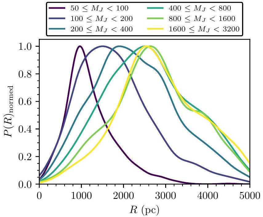
كاختبار أولي، الـ توزيع الكتل عند تقسيمها إلى صناديق كتلة منفصلة في الشكل 12 يظهر علامات واضحة على عدم الاكتمال اعتمادًا على كتلة الكتلة، حيث من المرجح أن تحدث الكتل ذات الكتلة المنخفضة عند مسافات منخفضة في كتالوجنا. في أدنى صندوق كتلة ( ، تصل ذروة توزيع الكتل عند بينما يصل إلى ذروته عندلأعلى فئتين من الكتلة و ). في أربع فئات الكتلة الأدنى، يبدو أنه خطي تقريبًا حتى يصل إلى ذروته، بعد ذلك تنخفض التوزيعة بشكل أسي. هذا هو النموذج المتوقع لتوزيع OC كما هو موضح في المعادلتين 4 و 5، مع الأخذ في الاعتبار بعض الحدود.نصف قطر الاكتمالفي كل كتلة معينة. من ناحية أخرى، لا تبدو أعلى صناديق الكتلة خطية حتى تصل إلى نصف قطرها الأقصى. قد يكون ذلك لأن العناقيد عالية الكتلة تبدو أكثر احتمالاً أن توجد في اتجاه مركز المجرة (انظر الشكل 7)، وأن افتراض أنافتراض أن التوزيع متساوٍ هو افتراض ضعيف.
لتحقيق توزيع الكتل دون تقسيم الكتلة، يوضح الشكل 13 الكتلة الكاملة- توزيع الكتل السماحية (OCs) تم تنعيمه باستخدام تقدير كثافة النواة. تم تطبيع تقديرات كثافة النواة بناءً على الكتلة، مما يعني فعليًا أن كل شريط عمودي في الشكل له قمة عند الواحد، مما يساعد على توضيح مكان ذروة التوزيع عند كتلة مجموعة معينة. تُظهر الاتجاهات في القمم علاقة لوغاريتمية خطية حتى كتلة ، بعد ذلك لا يرتفع التوزيع أكثر. وهذا يشير إلى أن هو الحد الأعلى التقريبي لـ Gaia الكمال. قد يكون ذلك بسبب عدة قيود في بيانات Gaia DR3 الحالية، مثل حد السطوع، ودقة القياسات الفلكية، والانقراض.
لتحديد هذه العلاقة، قمنا بتطبيق نموذج لوغاريتمي خطي مع نقطة انكسار بعده يصبح النموذج مسطحًا على قمم هذا التوزيع من. هذا يعطي التقريبحد الاكتمال لتعدادنا السكاني في OC، مع النموذج الذي يتخذ الشكل:
الشكل 14. دالة العمر المصححة من حيث الاكتمال للأجسام القريبة (OCs) في هذا العمل (نقاط سوداء) مقارنةً مع دوال العمر المختلفة في الأدبيات. الخطوط المتقطعة تظهر ملاءمات قانون القوة المكسور بينما الخطوط المنقطة تظهر ملاءمات دالة شكتير. تم تطبيع دوال العمر في الأدبيات إلى أعمار أقل من 0.2 مليار سنة لتسهيل تصور الفروق في شكل الطرف العلوي من التوزيعات. الخطوط الزرقاء تظهر الملاءمات من كرمولز وآخرون (2019)، والخطوط البرتقالية من أندرس وآخرون (2021)، والخطوط الحمراء هي الملاءمات من هذا العمل. تشير أشرطة الخطأ إلى عدم اليقين بواسون في البيانات. ملاءمات دالة شكتير من كرمولز وآخرون (2019) وأندرس وآخرون (2021) لها أعمار نموذجية مقاسة بعامللتصحيح خطأ في أكواد ملاءمة دالة شختير.
حيث القيدتم تطبيقه أيضًا أثناء التركيب. كانت أفضل ملاءمة لدينا تحتوي على قيم 39.5٪ ، و .
هذا النموذج يتعارض بوضوح مع ادعاء خارشينكو وآخرين (2013)، الذين زعموا أن تعداد العناقيد المفتوحة مكتمل ضمن 1.8 كيلو فرسخ. ضمن 1.8 كيلو فرسخ، فإن تعدادنا للعناقيد المفتوحة في السماء بالكامل مكتمل فقط للعناقيد الأثقل من – كتلة عنقودية مشابهة لتلك الخاصة بـ Melotte 25 (الهيديس). كتالوجنا مكتمل فقط ضمن 1 كيلوبارسيخ للعناقيد الأثقل من.
5.2. تقدير وظائف العمر والكتلة للعناقيد المفتوحة في درب التبانة
باستخدام تقدير الاكتمال التقريبي في القسم 5.1، من الممكن أيضًا تقدير دوال العمر والكتلة للعناقيد المفتوحة في مجرة درب التبانة من كثافة عدد العناقيد المفتوحة كدالة للعمر أو الكتلة، بالإضافة إلى العدد الإجمالي للعناقيد المفتوحة في مجرة درب التبانة. للقيام بذلك، يتم حساب عدد العناقيد المفتوحة على مسافات أقل منتم عد الكتلة المعطاة في صناديق، ثم قُسمت على المساحة الكلية ثنائية الأبعاد لدائرة نصف قطرهافي الكتلة المركزية لكل حاوية.
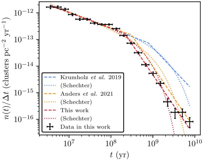
تم رسم دالة العمر المصححة للكمال للتجمعات النجمية في مجرة درب التبانة في الشكل 14. على عكس كرمولز وآخرون (2019) وأندرس وآخرون (2021)، الذين وجدوا أن دالة عمر التجمعات تُقارب بشكل جيد بواسطة قانون القوة المكسور أو دالة شكتير، نجد أن دالة عمر تجمعاتنا تتناسب بشكل جيد فقط مع قانون القوة المكسور، مع وجود ‘ركبة’ أكثر حدة في دالة عمر تجمعاتنا مقارنة بتلك الخاصة بأندرس وآخرون (2021) أو كرمولز وآخرون (2019). قد يكون هذا بسبب تعريفنا المختلف للتجمع النجمي من حيث إمكانيته الجاذبية، مما قد يعني أن كتالوجنا قد تم تنظيفه بشكل أقوى من التجمعات النجمية القديمة غير المرتبطة. ومع ذلك، نؤكد نتائج أندرس وآخرون.
الشكل 15. دالة الكتلة للأجسام المفتوحة في هذا العمل. الأعلى: دالة الكتلة المصححة من حيث الاكتمال للأجسام المفتوحة في هذا العمل (نقاط سوداء) مقارنةً بـقانون القوة (Krumholz et al. 2019، الخط المنقط الأزرق) مناسب للتجمعات ذات الكتل الأكبر من. الأسفل: دوال الكتلة المصححة للكمال للتجمعات، مفصولة حسب فئات العمر وتتضمن ملاءمات القوة لكل فئة عمرية.
(2021)، الذين وجدوا أن عدد العناقيد القديمة في غايا أقل بكثير من النتائج السابقة قبل غايا مثل بيشكينوف وآخرون (2018). بناءً على نتائجنا في الورقة الثانية، من المحتمل أن العدد المنخفض من العناقيد القديمة المستخلصة من غايا (بما في ذلك هذا العمل) يرجع إلى أن العديد من العناقيد القديمة المبلغ عنها قبل غايا من غير المحتمل أن تكون حقيقية. إن ملاءمتنا لقانون القوة المكسور لبياناتنا تعطي، ومع نقطة توقف عند تمتاز انحدارات هذا التوزيع بالتوافق ضمن حدود عدم اليقين مع نتائج أندرس وآخرين (2021)، على الرغم من أنأقل قليلاً من قيمتهم لـ.
الرسم العلوي من الشكل 15 يظهر دالة الكتلة المصححة من حيث الاكتمال للعناقيد المفتوحة في درب التبانة. فوق كتلة تبلغ حوالي، يتم تقريب هذه الدالة الكتلية بشكل جيد بواسطة قانون القوة مع مؤشر، وهو مطابق لدالة الكتلة الأولية للتجمعات الموجودة في العديد من المجرات الأخرى التي يتم تقريبها بشكل جيد بواسطة قانون القوة مع ميلللمجموعات ذات الكتل الأقل من (Portegies Zwart وآخرون 2010، Krumholz وآخرون 2019)، مما يعني معدل تشكيل العناقيد بشكل لوغاريتمي موحد كدالة للكتلة. ومع ذلك، بالنسبة للعناقيد التي تقل كتلتها عن نجد أن دالة القوة الأقل انحدارًا قليلاً هي أفضل ملاءمة للبيانات. يبدو أن هذا اتجاه يعتمد على العمر. يُظهر الرسم البياني السفلي من الشكل 15 الكتلة المجمعة حسب العمر.
الشكل 16. ميل التناسبات ذات القوة في الشكل 15 كدالة للعمر. ملاءمة لهذا الميل معمثبت عند -2 يظهر باللون الأزرق، مع ملاءمة معمجاني موضح باللون البرتقالي.
الشكل 17. العدد الإجمالي المقدر للأجسام القابلة للاكتشاف في درب التبانة مصححًا من حيث الاكتمال كدالة للكتلةبما في ذلك عدم اليقين من بواسون على الحاويات، مقارنة بتوزيع كتل OC في هذا العمل (باللون البرتقالي).
وظيفة نفس الكتل، بما في ذلك التناسبات بواسطة قوانين القوة غير المنكسرة. بالنسبة لأحدث الكتل، فإن دالة الكتلة الخاصة بها قريبة منقانون القوة، وهو التنبؤ للمجموعات الشابة في كرمولز وآخرون (2019). مع زيادة العمر، يبدو أن دالة كتلة المجموعة تتسطح، بالإضافة إلى انخفاضها عند جميع الكتل. قد تشير هذه التسطيحات في انحدارات دالة الكتلة مع العمر إلى تسريع في انحلال المجموعات ذات الكتلة المنخفضة كدالة للعمر مقارنة بالمجموعات ذات الكتلة العالية، ويجب التحقيق في ذلك من خلال دراسات نظرية.
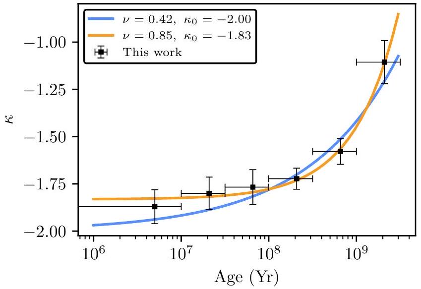
تظهر الشكل 16 انحدارات ملاءمات قانون القوة لدالة الكتلة المجمعة حسب العمر. نحن نلائم قوانين القوة المنحرفة بالشكللهذا التوزيع؛ أولاً، من أجلثابت عند -2، كما تم التنبؤ به لمجموعات العمر الصفري (كرومهولز وآخرون 2019)؛ وثانيًا، مع جميع المعلمات حرة. في الأولى (الحالة (ثابتة) ، نجد; في الحالة الثانية، نجد و يجب مقارنة هذه الملاحظات بمحاكاة N-body على نطاق واسع لذوبان العناقيد في المستقبل.
كما استخدمنا كثافة عدد الكتل المستمدة لدينا لحساب تقدير لإجمالي عدد العناقيد المفتوحة في درب التبانة عند كتلة معينة،، بافتراض توزيع قرصي مسطح للكتل المفتوحة بقطر 12.5 كيلو فرسخ فلكي، والذي يتوافق مع الحد التقريبي الذي تُلاحظ فيه الكتل المفتوحة في القرص المجري (انظر على سبيل المثال، الشكل 7). يوضح الشكل 17 العدد الإجمالي للكتل النجمية في هذا العمل مقارنةً بالتقدير الإجمالي للكتل النجمية في مجرة درب التبانة بعد تصحيح الاكتمال. من خلال جمع هذه التوزيعة، نقدر أن مجرة درب التبانة تحتوي على إجماليالأجسام السماوية ذات الكتل في النطاقالذي يمكن مقارنته بـتُقدّر الكتل النجمية في درب التبانة التي قد توجد وفقًا لدياز وآخرين (2002). هذا العدد الإجمالي المقدر يعني أن حوالي فقطعدد العناقيد المفتوحة في مجرة درب التبانة المعروف في الوقت الحالي، مع كون هذه النقصان أقوى بالنسبة للعناقيد ذات الكتلة المنخفضة.
جمع توقعاتناالتوزيع، نقدر أن درب التبانة تحتوي علىمن النجوم التي ترتبط حاليًا بالعناقيد المفتوحة. استخدم كاوتون وآخرون (2020) بيانات غايا DR2 لتقدير أن مجرة درب التبانة تحتوي علىمن الكتلة النجمية؛ مقارنة بتوقعاتنا، يشير هذا إلى أن حواليمن نجوم درب التبانة موجودة حاليًا في تجمع مفتوح. هذا مشابه للنسبة بين إجمالي عدد النجوم المدخلة لدينا في الورقة الثانية والعدد النهائي من النجوم التي نجد أنها مرتبطة حاليًا بتجمع مفتوح. في الورقة الثانية، استخدمنا قائمة مدخلة تضم 729 مليون نجم من بيانات غايا DR3 لبناء كتالوجنا. في هذا العمل، نجد أن 614358 من تلك النجوم موجودة حاليًا ضمن نصف قطر جاكوبى لتجمع مفتوح، والذي يبلغ حواليمن النجوم التي تم اعتبارها في تحليل التجميع في ورقتنا الثانية.
5.3. مقارنة بين دوال كتلة العنقود و IMF كروب
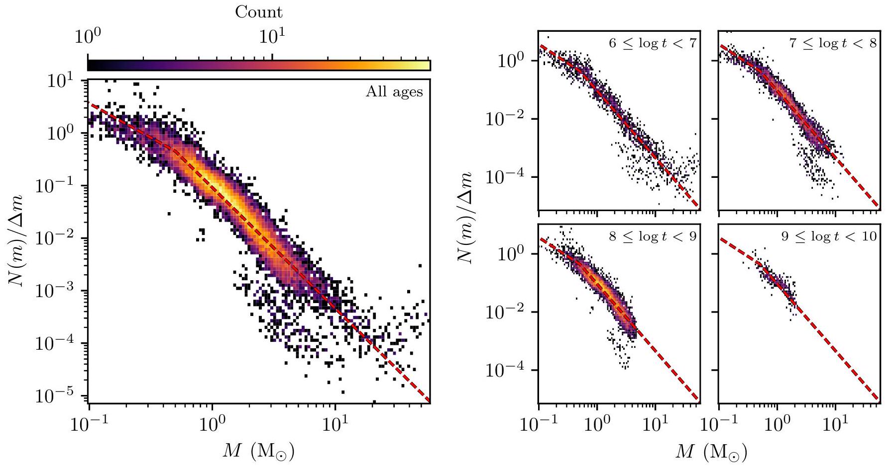
طوال هذا العمل، اعتمدنا على دالة الكتلة الأولية لكروب (Kroupa IMF) لحساب الكتل الإجمالية للعناقيد. بعد تصحيح شامل لتأثيرات اختيار عضوية العنقود في القسم 3.2، نجد أن دوال كتلة العنقود كانت متوافقة على نطاق واسع مع دالة الكتلة الأولية لكروب، وعبر مجموعة واسعة من أعمار العناقيد. توضح الشكل 18 نقاط البيانات من جميع دوال الكتلة في هذا العمل والمخططة كهيستوغرام ثنائي الأبعاد.
هناك بعض النقاط البارزة في هذه الصورة التي تستحق المناقشة في البداية. أولاً، النقاط ذات الكتلة الأعلى (مع كتل أكبر منيبدو أن الأعداد المبالغ فيها. وذلك لأن أعمار المجموعات من الورقة الثانية لها حد أدنى من، مما يعني أن النجوم ذات الكتلة العالية في تجمعات النجوم التي تقل أعمارها عن هذا العمر لا يمكن أن تكون لها كتل أعلى من هذا الحد المخصص لها، وبالتالي فإن أعلى فئات الكتلة في التجمعات الشابة يتم تقديرها بشكل مبالغ فيه بسبب التلوث من نجوم O ذات الكتلة الأعلى والأقصر عمراً. هذا واضح في subplot من الشكل – فقط العناقيد الشابة لديها هذه القياسات العالية بشكل خاطئ.
ثانيًا، بعض صناديق الكتلة في النطاقلأن بعض المجموعات تحتوي على عدد أقل بحوالي مرتبة من الحجم من النجوم مما كان متوقعًا لهذه المجموعات. تحتوي هذه الفئات ذات العدد المنخفض على عدم يقين بواسون مرتفع بشكل متناسب، ولا تغير بشكل كبير قياسات الكتلة الإجمالية للمجموعات، لكنها لا تزال تستحق المناقشة. من المحتمل أن تكون هناك أسباب متعددة لغياب النجوم عالية الكتلة في هذه المجموعات، بما في ذلك جودة منخفضة لرسوم CMD، إحصائيات عددية صغيرة، ملاءمة ضعيفة للخطوط الزمنية، وتأثيرات اختيار غير محسوبة. 902 من 6956 ( ) من العناقيد التي تحتوي على قياسات الكتلة في هذا العمل لديها على الأقل حاوية كتلة واحدة أكثر من أقل من القيمة المتوقعة من دالة توزيع كروبا، وبالتالي لديها نقاط ضمن المنطقة المحددة سابقًا. 200 من هذه العناقيد لديها مخططات CMD ذات جودة منخفضة (درجة CMD في الورقة الثانية أقل من 0.5) مما قد يعني أنها ليست مجموعة حقيقية واحدة من النجوم أو أنها اكتشاف ضعيف لعناقيد حقيقية، والتي قد تحتوي بالتالي على فجوات لأسباب غير فيزيائية.
من بين 702 مجموعة المتبقية ذات مخططات CMD عالية الجودة، تحتوي 572 على أقل من 100 نجم عضو، مما قد يكون معقولاً أن يكون لديها
الشكل 18. مقارنة بين نقاط دالة الكتلة للعناقيد في هذا العمل ودالة الكتلة لكروب. اليسار: مخططات ثنائية الأبعاد لجميع النقاط من جميع دوال الكتلة للعناقيد في هذا العمل لـ 1235 عنقود نجمي ضمن 2 كيلوبكسل في العينة عالية الجودة من العناقيد وذات 50 نجمًا عضوًا على الأقل، مقارنة بدالة الكتلة لكروب (الخط الأحمر المتقطع). يتم تطبيع دوال الكتلة الفردية للعناقيد قبل الدمج. لون صناديق المخطط البياني يدل على عدد نقاط دالة الكتلة التي دخلت في كل صندوق فردي، وفقًا لشريط الألوان في الزاوية العليا اليمنى. اليمين: نفس ما في اللوحة اليسرى، باستثناء أن العناقيد مقسمة إلى أربع فئات عمرية منفصلة.
الفجوات ببساطة بسبب النجوم المفقودة نتيجة إحصائيات عدد صغير، أو بسبب عدد قليل من النجوم مما يجعل من الصعب تحديد ملاءمة الإيزوكرون بدقة، حيث إن دقة استنتاج معلمات ورقتنا الثانية مرتبطة ارتباطًا وثيقًا بعدد النجوم الأعضاء. تقريبًا جميع نقاط دالة الكتلة المنخفضة بشكل خاطئ تقع في طرف التسلسل الرئيسي داخل العناقيد – وهي منطقة داخل CMD للعناقيد تكون عادةً ذات كثافة سكانية منخفضة ولكنها تغطي نطاقًا واسعًا من الكتل النجمية، خاصةً للعناقيد الشابة – مما يعني أن خطأ صغيرًا في ملاءمة الإيزوكرون أو في الإيزوكرون نفسه يمكن أن يت correspond إلى خطأ كبير في الكتلة النجمية المستنتجة، وبالتالي خلق مظهر فجوة في دالة الكتلة المقاسة لعناقيد.
ومع ذلك، لا تزال 54 مجموعة ذات مخططات CMD عالية الجودة و200 نجم عضو على الأقل تعاني من فجوات في دالة الكتلة. معظم هذه المجموعات قريبة. )، شاب ( )، ولديها معلمات فوتومترية مستنتجة بشكل جيد. جميع الفجوات في هذه المجموعات باستثناء واحدة أكثر سطوعًا من “، تكون عند أو بالقرب من طرف التسلسل الرئيسي، وتحدث في تجمعات مدروسة جيدًا مثل بلانكو 1 (، انظر الشكل 2). في حالة بلانكو 1، يبدو أن هذه الفجوة قوية بين الأعمال المختلفة، حيث تظهر في أعمال أخرى تعتمد على بيانات غايا (مثل زانغ وآخرون 2020؛ كانتات-غودين وآخرون 2020). قد تكون الفجوات عند درجات سطوع أعلى ذات دلالة لثلاثة أسباب. أولاً، تصبح أجهزة الاستشعار CCD الخاصة بغايا مشبعة فوق، وتخضع المصادر التي تتجاوز هذا الحد لعمليات معالجة فوتومترية مختلفة (رييلو وآخرون 2021). غالبًا ما تحتوي المصادر الساطعة في غايا على أخطاء استرومترية أعلى بكثير، مما قد يعني أنه تم استبعادها من قائمة عضوية العنقود بسبب ضعف الاسترومترية، أو أنها قد تحتوي فقط على حل استرومترية ذو معاملين وبالتالي لم يتم تضمينها في تحليل التجميع الخاص بنا، أو أنها أكثر عرضة لأن تُصنف كإيجابية زائفة بواسطة الطريقة التي استخدمها ريبزكي وآخرون (2022) لتنظيف مجموعة بيانات غايا DR3 في الورقة الثانية. ثانيًا، عند السطوع العالي، هناك إشارات- عدد أقل بكثير من النجوم، مما يعني أن وظيفة اختيار غايا أكثر صعوبة في التوصيف الدقيق تجريبيًا. قد يؤثر ذلك على وظائف اختيار غايا أو العينة الفرعية المطبقة في القسم 3.2. مع وجود عدد قليل فقط من النجوم في نطاق سطوع واسع معين لاستخدامه لتحديد وظيفة اختيار تجريبية، فإن عدم اليقين في وظيفة الاختيار في نطاق معين يكون أعلى. من الجدير بالذكر أنه في الشكل 2، فإن وظيفة اختيار العينة الفرعية لبلانكو 1 أقل في النطاق الذي يوجد فيه فجوة، مما يشير إلى أن أحد أسباب فقدان النجوم في هذا النطاق قد يكون تأثير اختيار مقدر بشكل غير دقيق. في المستقبل، قد يكون من الضروري تحسين وظائف اختيار العينة الفرعية بشكل أكبر لتكون أكثر دقة عند السطوع العالي حيث يجعل وجود عدد قليل من النجوم الساطعة في معظم الحقول من الصعب تحديد وظائف اختيار العينة الفرعية للنجوم الساطعة بدقة. أخيرًا، نظرًا لأن النجوم في نطاق الكتلةعادة ما تكون ثنائية (مو ودي ستيفانو 2017)، قد يكون أيضًا أن الأخطاء الأسترو مترية الناتجة عن النجوم الثنائية تسبب في فقدان بعض النجوم من قوائم عضويتنا في العنقود – خاصة إذا كانت علىيدور العام بحركة مشابهة لحركة المنظور (Lindegren et al. 2021). ستساعد تحسينات قياسات النجوم الثنائية وتصنيفاتها في Gaia DR4 على تقليل عدد النجوم الثنائية التي تم تجاهلها في الأعمال المستقبلية (Gaia Collaboration et al. 2023).
بعيدًا عن هذه النقاط الشاذة، فإن غالبية النقاط في دوال الكتلة العنقودية تتناسب جيدًا مع دالة الكتلة الأولية لكروب. يظهر بعض الانحراف عن دالة الكتلة الأولية لكروب في أقدم العناقيد في الشكل 18، حيث تبدو دوال الكتلة أكثر تسطحًا، مع احتمال أن يكون السبب الفيزيائي هو فقدان الكتلة المفضل للنجوم منخفضة الكتلة في أقدم العناقيد. ومع ذلك، فإننا غير قادرين أساسًا على إعادة إنتاج نتائج الأعمال التي تشمل كوردوني وآخرون (2023)، الذين يجدون أن دوال الكتلة العنقودية متوافقة مع انحدارات قانون القوة التي تنحرف بشكل كبير عن دالة الكتلة الأولية لكروب. للتحقيق في كتلة العنقود وظائف الكتلة العنقودية في المستقبل، وبدقة أعلى مما كان ممكنًا في هذا العمل، يجب إجراء وظائف الكتلة العنقودية التي تتضمن تصحيحات ثنائية النجوم من كتلة إلى أخرى بدقة أكبر. من المحتمل أن يكون ذلك ممكنًا مع المسوحات المستقبلية مثل Gaia DR4، التي ستوفر قياسات زمنية أفضل لتحديد الثنائيات (تعاون غايا وآخرون 2023)، أو باستخدام طيف النجوم في المسوحات الطيفية الكبيرة القادمة مثل 4MOST (دي يونغ وآخرون 2012) لتحديد الثنائيات الطيفية. حاليًا، فإن التعرف الفوتومتري على الثنائيات باستخدام بيانات غايا قادر فقط على اكتشاف النجوم الثنائية ذات نسبة الكتلة الأعلى.في أكثر التجمعات موثوقية (مثل كوردوني وآخرون 2023، دونادا وآخرون 2023).
6. الخاتمة
في هذا العمل، قمنا بالتحقيق في طرق لتصنيف تجمعات النجوم في درب التبانة على أنها مرتبطة أو غير مرتبطة. من خلال قياس كتل التجمعات وأشعة جاكوب، تمكنا من تصنيف 6956 تجمعًا من كتالوج تجمعات النجوم لدينا في الورقة الثانية على أنها تجمعات مرتبطة أو تجمعات غير مرتبطة. توفر هذه الطريقة في التصنيف وسيلة جديدة وأكثر دقة للتمييز بين التجمعات المرتبطة والتجمعات غير المرتبطة في بيانات غايا مقارنةً باستخدام قطع فردية على المعلمات.
كجزء من هذا العمل، نُصدر كتالوجًا لكتل وأحجام تجمعات النجوم، وهو أكبر كتالوج لكتل تجمعات درب التبانة حتى الآن، حيث أنه أكبر بحوالي سبع مرات من أكبر كتالوج لكتل تجمعات النجوم المفتوحة الذي تم إعداده باستخدام بيانات غايا حتى الآن (ألmeida وآخرون 2023). تم حساب كتل تجمعاتنا بدقة من خلال أخذ ثلاثة تأثيرات اختيارية في مخططات الألوان والسطوع في الاعتبار وتأثير الثنائيات غير المحلولة. نقارن تقديرات كتلنا بتلك الموجودة في الأدبيات، ونجد أن كتلنا عادة ما تكون أعلى من نتائج الأدبيات السابقة. نقترح أن هذا يعود إلى تضميننا تصحيحات تأثيرات الاختيار.
نستخدم كتل العناقيد لدينا لتقدير نسبة العناقيد من الورقة الثانية التي تتوافق مع الأجسام المرتبطة (التي تتجاذب ذاتيًا على الفور)، وننشر كتالوجًا محدثًا للعناقيد النجمية مع تصنيفات محسّنة للعناقيد. ضمن 15 كيلو فرسخ (أقصى مسافة نقدم لها قياسات الكتلة)، نجد أن فقطالعناقيد من الورقة الثانية متوافقة مع كونها مرتبطة. بالقرب من الشمس، ضمن 250 فرسخ فلكي، يهيمن على كتالوجنا النجوم المتحركة، مع فقطتتعلق الكتل المتوافقة مع الأجسام المقيدة. يحتوي كتالوجنا النهائي على 5647 تجمعًا نجميًا، 3530 منها في عينة عالية الجودة مع نسبة إشارة إلى ضوضاء فلكية أعلى ومخططات CMDs جيدة الجودة. يحتوي الكتالوج على 1309 مجموعات نجمية، 539 منها عالية الجودة بنفس التعريف.
تظهر المقارنات بين العناقيد المفتوحة (OCs) والعناقيد الكروية (MGs) في كتالوجنا اختلافات مثيرة بين هذه الأجسام. التركيز الهيكلي للعناقيد المفتوحة يعتمد بشكل كبير على كتلتها، وليس على عمرها. من ناحية أخرى، فإن العناقيد الكروية الأقدم أكبر بكثير من العناقيد الشابة، وهو ما يتوافق مع كونها أجسام غير مرتبطة وتتمدد. يبدو أن العناقيد الكروية الشابة والعناقيد المفتوحة في كتالوجنا تتشكل بأحجام ابتدائية مشابهة، ولكن مع تمدد العناقيد الكروية بشكل أكبر مع تقدم العمر. كانت اكتشافنا للعديد من العناقيد الكروية في بحثنا عن العناقيد في الورقة الثانية حادثة، حيث كنا نعتزم فقط اكتشاف العناقيد المفتوحة؛ ومع ذلك، نظرًا لأن كل من العناقيد الكروية والعناقيد المفتوحة هي بقايا لتكوين النجوم المتزامن، وقد تكون بعض العناقيد الكروية غير المرتبطة حتى بقايا لعناقيد مفتوحة مرتبطة، سيكون من المنطقي في عمليات البحث المستقبلية عن العناقيد العمياء الاستمرار في البحث عن كلا الفئتين من الأجسام وإجراء مقارنات بينهما.
استخدمنا هذه النتائج أيضًا لاشتقاق تقديرات تقريبية للاكتمال، ودالة العمر، ودالة الكتلة لتعداد العناقيد المفتوحة في بيانات غايا DR3. يتم وصف اكتمال كتالوجنا بشكل جيد بواسطة دالة لوغاريتمية تعتمد فقط على كتلة العنقود حتى ، وراء ذلك حد الاكتمال لا يزيد أكثر. ذكر خارشينكو وآخرون (2013) أن تعداد العناقيد المفتوحة مكتمل ضمن 1.8 كيلوبارسيك، وهو ادعاء تم دحضه منذ ذلك الحين من قبل العديد من الأعمال المستندة إلى بيانات غايا (كاسترو-جينارد وآخرون 2018، 2019، 2020، 2022؛ ليو وبانغ 2019؛ سيم وآخرون 2019؛ هانت وريفيرت 2021، 2023)؛ في هذا العمل، نجد أن تعداد العناقيد المفتوحة لدينا هو فقط تقريبًااكتمل عند 1.8 كيلو فرسخ فلكي للتجمعات الأثقل من، مما يشير إلى أن العديد من العناقيد المفتوحة ذات الكتلة المنخفضة لا تزال بحاجة إلى الاكتشاف ضمن هذه المسافة.
باستخدام هذا التقدير للاكتمال، نؤكد نتائج أندرس وآخرين (2021) بأن إحصاء غايا للكتل المفتوحة (OCs) هو أصغر سناً بشكل ملحوظ من الأعمال السابقة على غايا. كما نستخرج دالة الكتلة المصححة للاكتمال من كتالوج الكتل المفتوحة لدينا، ونجد أن الكتل المفتوحة التي تزيد عن حواليمتوافقة مع قانون القوة بزاوية ميل تساوي -2، وهو ما يتوافق مع ملاحظات دالة كتلة العنقود للعديد من المجرات الأخرى (كرومهولز وآخرون 2019). ومع ذلك، نجد أنه تحت هذه الكتلة، هناك عدد أقل من المجموعات مما هو متوقع. مقسمة إلى فئات عمرية، يبدو أن دالة كتلة مجموعتنا تتسطح مع زيادة العمر، مما يشير إلى معدل متسارع من تفكك المجموعات للمجموعات ذات الكتلة المنخفضة. تشير دالة كتلة مجموعتنا إلى أن درب التبانة يجب أن تحتوي على إجمالي حواليالتي تعرف حاليًا. أخيرًا، في دراسة دوال الكتلة للعناقيد الفردية، نجد أن معظم العناقيد المفتوحة تتوافق بشكل عام مع دالة الكتلة الأولية لكروبّا للأعمار التي تقل عن 1 مليار سنة – ولكن فقط بعد تصحيح شامل لدوال كتلتها لتأثيرات الاختيار.
منذ إصدار بيانات غايا DR2 (براون وآخرون 2018)، حدث انفجار في الدراسات التي تُبلغ عن اكتشافات جديدة لمجموعات النجوم المفتوحة (مثل سيم وآخرون 2019؛ كاسترو-جينارد وآخرون 2020، 2022، ليو وبانغ 2019، هي وآخرون 2021، 2022؛ هاو وآخرون 2022). تتفق الأعمال عمومًا على أن مجموعة النجوم المفتوحة يجب أن تكون كثافة زائدة في بيانات غايا، مع وجود على الأقلنجوم الأعضاء، وCMD متوافق مع مجموعة واحدة من النجوم. ومع ذلك، حتى الآن، لم يكن هناك وسيلة لتعريف مجموعات النجوم المكتشفة بشكل أكبر إلى كائنات مرتبطة وغير مرتبطة من خلال الملاحظات. ستعمل فعالية قياس أنصاف أقطار جاكوبى للمجموعات لهذا الغرض على تحسين دقة ووضوح كل من التعداد الحالي لمجموعات النجوم المفتوحة والتعدادات المستقبلية لمجموعات النجوم المفتوحة استنادًا إلى إصدارات البيانات القادمة.
الشكر والتقدير. نشكر المحكم المجهول على تعليقاتهم التي حسنت جودة هذه الورقة، وكذلك سيغفريد ريسر وإلينا شيلباخ على تعليقاتهم المفيدة الأخرى. يقر كل من إ.ل.هـ. وس.ر. بامتنان بتمويل من مؤسسة الأبحاث الألمانية (DFG) – رقم المشروع 138713538 – SFB 881 (“نظام درب التبانة”، المشروع الفرعي B5). نشكر خوسيفا غروشفيدل، برونو أليسي، فيليب توتش، سيغفريد ريسر، وإلينا شيلباخ على تقديم ملاحظات حول العناقيد غير الموثوقة أو الأسماء الرئيسية من عملنا في الورقة الثانية. لقد استخدم هذا العمل بيانات من مهمة وكالة الفضاء الأوروبية (ESA) غايا.https://www. cosmos.esa.int/gaia)، المعالجة بواسطة اتحاد معالجة وتحليل بيانات غايا (DPAC،https://www.cosmos.esa.int/web/gaia/dpac/الاتحاد. تم توفير التمويل لـ DPAC من قبل المؤسسات الوطنية، وخاصة المؤسسات المشاركة في الاتفاقية متعددة الأطراف غايا. استخدمت هذه الأبحاث نظام بيانات ناسا لعلم الفلك وخدمات الببليوغرافيا. كما استخدمت هذه الأبحاث قاعدة بيانات SIMBAD، التي تُدار في CDS، ستراسبورغ، فرنسا (وينجر، م. وآخرون 2000). بالإضافة إلى ما تم ذكره في النص الرئيسي، استخدمت هذه العمل حزم بايثون مفتوحة المصدر NumPy (هاريس وآخرون 2020)، SciPy (فيرتانين وآخرون 2020)، IPython (بيريز وغرانجر 2007)، Jupyter (كلويفر وآخرون 2016)، Matplotlib (هانتر 2007)، pandas (ماكينى 2010. فريق تطوير pandas 2020. و Astropy (روبيتايل وآخرون 2013، تعاون Astropy وآخرون 2018). كما استخدمت هذه العمل دورات ألوان مشابهة لـ Matplotlib المتاحة كما هو محدد في بيتروف (2021).
References
Akeson, R. L., Chen, X., Ciardi, D., et al. 2013, PASP, 125, 989
Almeida, A., Monteiro, H., & Dias, W. S. 2023, MNRAS, 525, 2315
Anders, F., Cantat-Gaudin, T., Quadrino-Lodoso, I., et al. 2021, A&A, 645
Astropy Collaboration, Price-Whelan, A. M., Sipőcz, B. M., et al. 2018, AJ, 156, 123
Banerjee, S. & Kroupa, P. 2017, A&A, 597, A28
Binney, J. & Tremaine, S. 1987, Galactic Dynamics (Princeton, N.J.: Princeton University Press)
Bossini, D., Vallenari, A., Bragaglia, A., et al. 2019, A&A, 623, A108
Bovy, J. 2015, ApJS, 216, 29
Bravi, L., Zari, E., Sacco, G. G., et al. 2018, A&A, 615, A37
Bressan, A., Marigo, P., Girardi, L., et al. 2012, MNRAS, 427, 127
Brown, A. G. A., Vallenari, A., Prusti, T., et al. 2018, A&A, 616, A1
Cahlon, S., Zucker, C., Goodman, A., Lada, C., & Alves, J. 2024, ApJ, 961, 153
Campello, R. J. G. B., Moulavi, D., & Sander, J. 2013, Adv. Knowl. Discov. Data Min., 7819, 160
Cantat-Gaudin, T. 2022, Universe, 8, 111
Cantat-Gaudin, T. & Anders, F. 2020, A&A, 633, A99
Cantat-Gaudin, T., Anders, F., Castro-Ginard, A., et al. 2020, A&A, 640, A1
Cantat-Gaudin, T., Fouesneau, M., Rix, H.-W., et al. 2023, A&A, 669, A55
Cantat-Gaudin, T., Jordi, C., Vallenari, A., et al. 2018, A&A, 618, A93
Cantat-Gaudin, T., Krone-Martins, A., Sedaghat, N., et al. 2019, A&A, 624, A126
Castro-Ginard, A., Brown, A. G. A., Kostrzewa-Rutkowska, Z., et al. 2023, A&A, 677
Castro-Ginard, A., Jordi, C., Luri, X., Cantat-Gaudin, T., & Balaguer-Núñez, L. 2019, A&A, 627
Castro-Ginard, A., Jordi, C., Luri, X., et al. 2022, A&A, 661, A118
Castro-Ginard, A., Jordi, C., Luri, X., et al. 2020, A&A, 635
Castro-Ginard, A., Jordi, C., Luri, X., et al. 2018, A&A, 618, A59
Castro-Ginard, A., McMillan, P. J., Luri, X., et al. 2021, A&A, 652, A162
Cautun, M., Benítez-Llambay, A., Deason, A. J., et al. 2020, MNRAS, 494, 4291
Choi, J., Dotter, A., Conroy, C., et al. 2016, ApJ, 823, 102
Colombo, D., Duarte-Cabral, A., Pettitt, A. R., et al. 2022, A&A, 658, A54
Cordoni, G., Milone, A. P., Marino, A. F., et al. 2023, A&A, 672, A29
de Jong, R. S., Bellido-Tirado, O., Chiappini, C., et al. 2012, in Society of PhotoOptical Instrumentation Engineers (SPIE) Conference Series, Vol. 8446, Proc. SPIE, eprint: arXiv:1206.6885, 84460T
Dias, W. S., Alessi, B. S., Moitinho, A., & Lépine, J. R. D. 2002, A&A, 389, 871
Donada, J., Anders, F., Jordi, C., et al. 2023, A&A, 675, A89
Ernst, A., Just, A., Berczik, P., & Olczak, C. 2011, A&A, 536, A64
Froebrich, D., Scholz, A., & Raftery, C. L. 2007, MNRAS, 374, 399
Gaia Collaboration, Brown, A. G. A., Vallenari, A., et al. 2021, A&A, 649, A1
Gaia Collaboration, Vallenari, A., Brown, A., Prusti, T., & et al. 2023, A&A, 674
Gran, F., Zoccali, M., Saviane, I., et al. 2022, MNRAS, 509, 4962
Hao, C. J., Xu, Y., Wu, Z. Y., et al. 2022, A&A, 660, A4
Harris, C. R., Millman, K. J., van der Walt, S. J., et al. 2020, Nature, 585, 357
He, Z., Liu, X., Luo, Y., Wang, K., & Jiang, Q. 2022, Astrophys. J. Suppl. Ser., 264, 8
He, Z.-H., Xu, Y., Hao, C.-J., Wu, Z.-Y., & Li, J.-J. 2021, Res. Astron. Astrophys., 21, 093
Hunt, E. L. 2023, Doctoral thesis, Universität Heidelberg, Heidelberg, Germany
Hunt, E. L. & Reffert, S. 2021, A&A, 646, A104
Hunt, E. L. & Reffert, S. 2023, A&A, 673, A114
Hunter, J. D. 2007, Comput. Sci. Eng., 9, 90
Just, A., Piskunov, A. E., Klos, J. H., Kovaleva, D. A., & Polyachenko, E. V. 2023, A&A, 672, A187
Kharchenko, N. V., Piskunov, A. E., Schilbach, E., Röser, S., & Scholz, R.-D. 2013, A&A, 558, A53
King, I. 1962, AJ, 67, 471
King, I. R. 1966, AJ, 71, 64
Kluyver, T., Ragan-Kelley, B., Pérez, F., et al. 2016, in Position. Power Acad. Publ. Play. Agents Agendas, ed. F. Loizides & B. Schmidt (IOS Press), 8790
Krause, M. G. H., Offner, S. S. R., Charbonnel, C., et al. 2020, Space Sci. Rev., 216, 64
Kronberger, M., Teutsch, P., Alessi, B., et al. 2006, A&A, 447, 921
Kroupa, P. 2001, MNRAS, 322, 231
Krumholz, M. R., McKee, C. F., & Bland-Hawthorn, J. 2019, Annu. Rev. Astron. Astrophys., 57, 227
Kuhn, M. A., Hillenbrand, L. A., Sills, A., Feigelson, E. D., & Getman, K. V. 2019, AJ, 870, 32
Lindegren, L., Klioner, S. A., Hernández, J., et al. 2021, A&A, 649, A2
Liu, L. & Pang, X. 2019, ApJS, 245, 32
McInnes, L., Healy, J., & Astels, S. 2017, JOSS, 2, 205
McKinney, W. 2010, in Proc. 9th Python Sci. Conf., Austin, Texas, 56-61
Meingast, S., Alves, J., & Rottensteiner, A. 2021, A&A, 645, A84
Moe, M. & Di Stefano, R. 2017, ApJS, 230
Moraux, E., Bouvier, J., Stauffer, J. R., & Cuillandre, J.-C. 2003, A&A, 400, 891
Oh, S. & Evans, N. W. 2020, MNRAS, 498, 1920
Pang, X., Li, Y., Yu, Z., et al. 2021, ApJ, 912, 162
Pérez, F. & Granger, B. E. 2007, Comput. Sci. Eng., 9, 21
Perren, G. I., Pera, M. S., Navone, H. D., & Vázquez, R. A. 2023, MNRAS, 526
Petroff, M. A. 2021, arXiv e-prints, 2107.02270
Piatti, A. E., Illesca, D. M. F., Massara, A. A., et al. 2023, MNRAS, 518, 6216
Piskunov, A. E., Just, A., Kharchenko, N. V., et al. 2018, A&A, 614, A22
Piskunov, A. E., Schilbach, E., Kharchenko, N. V., Röser, S., & Scholz, R.-D. 2008, A&A, 477, 165
Platais, I., Kozhurina-Platais, V., & van Leeuwen, F. 1998, AJ, 116, 2423
Plummer, H. C. 1911, MNRAS, 71, 460
Portegies Zwart, S. F., McMillan, S. L. W., & Gieles, M. 2010, Annu. Rev. Astron. Astrophys., 48, 431
Riello, M., De Angeli, F., Evans, D. W., et al. 2021, A&A, 649, A3
Rix, H.-W., Hogg, D. W., Boubert, D., et al. 2021, AJ, 162, 142
Robitaille, T. P., Tollerud, E. J., Greenfield, P., et al. 2013, A&A, 558, A33
Rybizki, J., Green, G., Rix, H.-W., et al. 2022, MNRAS, 510, 2597
Sim, G., Lee, S. H., Ann, H. B., & Kim, S. 2019, J. Korean Astron. Soc., 52, 145
Spina, L., Magrini, L., & Cunha, K. 2022, Universe, 8, 87
The pandas development team. 2020, Pandas-Dev/Pandas: Pandas, Zenodo
Vasiliev, E. & Baumgardt, H. 2021, MNRAS, 505, 5978
Virtanen, P., Gommers, R., Oliphant, T. E., et al. 2020, Nature Methods, 17, 261
Wenger, M., Ochsenbein, F., Egret, D., et al. 2000, Astron. Astrophys. Suppl. Ser., 143, 9
Zhang, Y., Tang, S.-Y., Chen, W. P., Pang, X., & Liu, J. Z. 2020, ApJ, 889
Zucker, C., Alves, J., Goodman, A., Meingast, S., & Galli, P. 2023, in Astronomical Society of the Pacific Conference Series, Vol. 534, Protostars Planets VII, ed. S. Inutsuka, Y. Aikawa, T. Muto, K. Tomida, & M. Tamura, 43
Zucker, C., Peek, J. E. G., & Loebman, S. 2022, ApJ, 936, 160
الملحق أ: تحديثات الأسماء
الجدول A.1. جميع تحديثات الأسماء المطبقة على الكتالوج.
III. Using cluster masses, radii, and dynamics to create a cleaned open cluster catalogue
Emily L. Hunt and Sabine Reffert Landessternwarte, Zentrum für Astronomie der Universität Heidelberg, Königstuhl 12, 69117 Heidelberg, Germanye-mail: ehunt@lsw.uni-heidelberg.de
Received 17 November 2023; accepted 5 March 2024
Abstract
Context. The census of open clusters has exploded in size thanks to data from the Gaia satellite. However, it is likely that many of these reported clusters are not gravitationally bound, making the open cluster census impractical for many scientific applications. Aims. We aim to test different physically motivated methods for distinguishing between bound and unbound clusters, using them to create a cleaned star cluster catalogue. Methods. We derived completeness-corrected photometric masses for 6956 clusters from our earlier work. Then, we used these masses to compute the size of the Roche surface of these clusters (their Jacobi radius) and distinguish between bound and unbound clusters. Results. We find that only of the clusters from our previous catalogue are compatible with bound open clusters, dropping to just of clusters within 250 pc. Our catalogue contains 3530 open clusters in a more strongly cut high-quality sample of objects. The moving groups in our sample show different trends in their size as a function of age and mass, suggesting that they are unbound and undergoing different dynamical processes. Our cluster mass measurements constitute the largest catalogue of Milky Way cluster masses to date, which we also use for further science. Firstly, we inferred the mass-dependent completeness limit of the open cluster census, showing that the census is complete within 1.8 kpc only for objects heavier than . Next, we derived a completenesscorrected age and mass function for our open cluster catalogue, including estimating that the Milky Way contains a total of open clusters, only of which are currently known. Finally, we show that most open clusters have mass functions compatible with the Kroupa initial mass function. Conclusions. We demonstrate Jacobi radii for distinguishing between bound and unbound star clusters, and publish an updated star cluster catalogue with masses and improved cluster classifications.
Key words. open clusters and associations: general – Methods: data analysis – Catalogs – Astrometry
1. Introduction
Data releases from the Gaia satellite have completely revolutionised the census of open clusters (OCs) (Cantat-Gaudin 2022). Since the first full Gaia data release (Brown et al. 2018), strides have been made in many aspects of the census, including ruling out many OCs reported before Gaia as asterisms (CantatGaudin & Anders 2020, Piatti et al. 2023, Hunt & Reffert 2021, 2023), detecting many thousands of new objects thanks to Gaia’s high-precision astrometry (e.g. Liu & Pang 2019; Castro-Ginard et al. 2020), and determining cluster parameters to higher levels of accuracy than previously possible (e.g. Bossini et al. 2019, Cantat-Gaudin et al. 2020). Nevertheless, the OC census still has room for improvement, with a major issue being that current observational definitions of OCs do not seem to be robust enough to distinguish them from unbound moving groups (MGs) (Hunt & Reffert 2023).
Cantat-Gaudin & Anders (2020) improve on the first major catalogue of OCs in the Gaia era, (Cantat-Gaudin et al. 2018), searching for additional OCs in Gaia data and using
a set of observational criteria to distinguish between plausible OCs and asterisms. Their criteria are as follows: firstly, a candidate OC should be a clear overdensity, including that it has at least roughly ten member stars; secondly, it must have a colourmagnitude diagram (CMD) that follows a clear isochrone, indicating that a given cluster is a co-evolutionary population of stars with the same age and chemical composition; and finally, a candidate OC must pass criteria that distinguish asterisms that cannot physically be gravitationally bound from potential bound OCs: namely, a median radius less than 15 pc , and a proper motion dispersion that corresponds to an internal velocity dispersion smaller than (or for distant clusters where Gaia measurement uncertainties are dominant.)
The criteria on the density (or number of stars) and CMD quality of an OC candidate are common practice in the literature. For instance, Froebrich et al. (2007), Cantat-Gaudin et al. (2019), and Hunt & Reffert (2021) (hereafter Paper I) require a candidate new cluster to be a clear overdensity, while works such as Platais et al. (1998), Castro-Ginard et al. (2018), and Liu & Pang (2019) are examples of works that use cluster CMDs to validate candidate new objects. The Cantat-Gaudin & Anders (2020) criteria on the possibility of a cluster being bound have also been adopted in the literature, with works such as Hunt &
Reffert (2021) and Castro-Ginard et al. (2022) using them to validate new OC candidates.
In Hunt & Reffert (2023) (hereafter Paper II), we used Gaia DR3 data (Gaia Collaboration et al. 2023) to construct a large, homogeneous catalogue of star clusters. However, despite our methodology being originally intended to only detect OCs, many of the clusters we detected appear to be MGs, often having sparse or ‘flat’ stellar distributions – unlike the clustered appearance of canonically bound OCs such as the Pleiades. Many of the suspected MGs we detected are consistent with being single populations of co-evolutionary stars based on our CMD classifier in Paper II, and most of the MGs we detected still pass the observational criteria on the boundness of an OC proposed in CantatGaudin & Anders (2020). In Paper II, we suggested that these criteria are too permissive to accurately classify the many sparse star clusters we are able to detect near to the Sun. The inability to distinguish precisely between bound and unbound clusters limits the scientific usability of catalogues such as the one in Paper II, with a significant proportion of the catalogue’s content being likely to be MGs – particularly within around 1 kpc from the Sun.
In this work, we aim to create a new way to distinguish between bound and unbound clusters, utilising a relationship between the mass and Jacobi radius of a self-gravitating cluster. With this method, we aim to classify all objects in Paper II into bound and unbound objects, in addition to demonstrating the applicability of this method to future studies of the Milky Way’s clusters, such as with upcoming data releases like Gaia DR4. Firstly, we provide an overview of some background theory in Sect 2. In Sect. 3, we outline how we calculate cluster masses and radii, including how we correct for selection effects and unresolved binary stars. Section 4 outlines the results of this work, including how many clusters in Paper II are bound OCs and how they are distributed. We explore the results of this work further in Sect. 5 , including using our cluster masses to estimate the massdependent completeness of the Gaia DR3 OC census, the age and mass functions of the OC census, and the compatibility of clusters with a Kroupa IMF (Kroupa 2001). Section 6 concludes this work.
2. Theoretical relations on the boundness of a cluster
In this section, we review some theory on how the boundness of a star cluster could be measured. We aim to find relations that can be straightforwardly applied to Gaia data of star clusters.
2.1. The virial theorem
One of the most common and widely used relations in astrophysics is the virial theorem, which states that a system under the influence of gravitation and in equilibrium should have twice as much kinetic energy as it has potential energy . For a star cluster with a distribution function following a Plummer (1911) model, this implies that a star cluster in virial equilibrium should have a one-dimensional velocity dispersion equal to an ideal virial velocity dispersion given by (Portegies Zwart et al. 2010): for a bound cluster,
where is the gravitational constant, is the cluster’s mass, is the cluster’s half-mass radius, and is a constant equal to for a typical cluster – although it can be as low as or as high as depending on the cluster’s spatial distribution (Portegies Zwart et al. 2010). This relation is used to analyse the dynamics of a small subset of nearby OCs in works including Bravi et al. (2018), Kuhn et al. (2019), and Pang et al. (2021).
Equation 1 may offer some explanation on why the individual empirical cuts presented in Cantat-Gaudin & Anders (2020) seem to be inadequate to distinguish between OCs and MGs from Paper II. As an example, consider a small cluster with a radius of and a velocity dispersion of around . Equation 1 predicts that this cluster would need a mass of to be virialised – a value far higher than almost all OCs in the Milky Way, and clearly unrealistic for typical small MGs that we detect in Paper II. Instead of adopting individual radius and velocity dispersion cuts, it appears that the expected radius and velocity dispersion of OCs must be ‘calibrated’ individually based on a cluster’s mass.
However, during the preparation of this work, we found this relation impossible to apply successfully to all clusters in Paper II. Velocity dispersions are easily contaminated by Gaia measurement uncertainties, binary stars, unbound stars (including stars in cluster tidal tails), perspective expansion, and interloping field stars. For instance, we found that binary stars (resolved or unresolved) often contribute or more to cluster velocity dispersions derived using proper motions, and incorrect removal of tidal tails can contribute as much as in the worst cases. In addition, Gaia measurement uncertainties become dominant in the proper motion dispersion of most clusters above a few kpc, making it difficult to make a meaningful measurement of for many clusters. Accounting for all of these effects for all clusters in Paper II and arriving at accurate measurements of was not possible. In addition, it is predicted theoretically that star clusters are often supervirial, such as during phases of expansion for young clusters (Banerjee & Kroupa 2017, Krause et al. 2020) – making it difficult to make a scientifically motivated cut on in many cases, as the velocity dispersion of many bound clusters can be expected to be supervirial, with measurements in multiple studies supporting this hypothesis (e.g. Bravi et al. 2018, Kuhn et al. 2019, Pang et al. 2021).
2.2. Jacobi radii
Using currently available data, we found it was much more successful to only rely on cluster masses and radii alone to distinguish between OCs and MGs. An instantaneously bound cluster should have a Roche surface, within which its potential is stronger than that of its host galaxy. In principle, a cluster with no radius at which its potential is stronger than that of the Milky Way will have no Roche surface, and is hence not selfgravitating. The Roche surface of a given cluster can be measured by considering its Jacobi radius, , which is the distance from the centre of a cluster to its Lagrange point. This is given by (Portegies Zwart et al. 2010, Ernst et al. 2011): ,
which relates to the mass of a cluster, weighted by the circular frequency and epicyclic frequency of the cluster’s orbit around its host galaxy, assuming that the orbit is circular. Outside of , the host galaxy’s potential is dominant – such as
Fig. 1. CMD of member stars of NGC 2451A shaded by their calculated stellar mass. 100 sampled isochrones for the cluster from Paper II are shown in black. (Adapted from Hunt 2023)
for stars in the tidal tails of a cluster, which are no longer bound to their parent cluster (Meingast et al. 2021). Assuming that a cluster fills its Roche surface, from a King (1962) model fit (Binney & Tremaine 1987), with this relationship being used by works such as Piskunov et al. (2008) to derive the masses of OCs based on their size.
Despite the fact that some open clusters, such as the Hyades, have been shown to have higher than expected stellar velocity dispersions and are supervirial and dissolving, these dissolving clusters are nevertheless dense enough to be currently selfgravitating (Oh & Evans 2020, Meingast et al. 2021). The same applies for young clusters that have recently been observed to be in possible supervirial expansion phases not long after their initial formation (Kuhn et al. 2019). On the other hand, MGs of all kinds (including sparse OB associations) are not bound, and are actively dissolving into the disk, meaning that they should have no radius at which they have a Roche sphere, which should be possible to measure with Eqn. 2 . For the remainder of this work, we aim to apply this equation to distinguish between bound and unbound star clusters.
3. Mass and radius calculations
In this section, we describe how we calculated photometric masses and Jacobi radii for all clusters within 15 kpc from Paper II. Much of this method was originally described in Hunt (2023), but is outlined again here to aid in the reading of this work. This method contains five steps that we discuss in the following subsections. Firstly, we derived the photometric masses of member stars in every cluster. Next, we corrected for selection effects. We then applied a correction for unresolved binary stars. Mass functions were then fitted and integrated to calculate total cluster mass. Finally, this process was repeated at different radii to find the Jacobi radius of each cluster.
3.1. Calculation of stellar masses
Following a similar method to that used by works including Meingast et al. (2021) and Cordoni et al. (2023), we began by using PARSEC (Bressan et al. 2012) isochrone fits from Paper II to
estimate the masses of member stars of each cluster. To calculate stellar masses, we used the predicted mass of stars as a function of -band magnitude from our fitted Paper II isochrones, , which was accurate for most cluster members. However, the oldest clusters in our sample often contain evolved giant stars whose -band magnitude is less than the tip of the main sequence in the cluster – meaning that is not a one-to-one mapping from magnitude to mass for some cluster members. Therefore, in regions where our fitted PARSEC isochrones do not have a one-to-one mapping from magnitude to mass, we also used colour indices to decide on the best stellar mass for a given cluster member. We elected not to use the index of most stars as and magnitudes are frequently underestimated for very red or blue stars with magnitudes (Riello et al. 2021). The regions where we do use colour indices were not within ranges where and are underestimated, however, due to the blue colour of these regions and due to our studied clusters being within 15 kpc .
To incorporate the uncertainty on our isochrone fits from Paper II, we repeated this process 100 times for 100 sampled isochrones from our variational inference neural network in Paper II. This incorporated uncertainties on the age, extinction, and distance to stars into our mass estimates for them. Figure 1 illustrates this process for NGC 2451A, showing 100 sampled isochrones from Paper II and our estimated stellar masses for each star with the shading of points.
It is worth discussing further the limitations and assumptions of this method. Firstly, since our Paper II photometric parameters do not include metallicities, our masses are biased for clusters with particularly low or high metallicities. To quantify this systematic, we repeated our entire pipeline on 143 randomly selected clusters but assuming metallicities of and -0.5 dex, testing how masses change given values at the upper and lower limit of those observed in OCs (Kharchenko et al. 2013; Bossini et al. 2019). Assuming a high metallicity increases masses by an average of , while a low metallicity decreases masses by an average of . The mean metallicity of OCs is approximately solar (Kharchenko et al. 2013), and so these values are edge-case limits that will mostly impact clusters at particularly high or low galactocentric radii which are most likely to have non-solar metallicities (Spina et al. 2022). In the future, it will be important to include spectroscopic metallicity estimates in machine learning OC parameter inference to improve the accuracy of OC masses further.
Next of note is that the effects of binary stars were not included in our interpolation scheme. Our stellar mass estimates are hence only estimates of the mass of the primary star in any binary system. To mitigate this effect, we applied a correction to the overall cluster mass function for unresolved binaries in Sect. 3.3
Finally, our use of PARSEC isochrones also influences our derived stellar masses, and our mass estimates may differ to those derived using other stellar evolution models. We investigated how using MIST isochrones (Choi et al. 2016) would change our mass estimates, using limited comparisons between our fitted PARSEC isochrones and MIST isochrones at the same age. for PARSEC and MIST isochrones is generally very similar for at all ages, and hence for clusters at distances greater than 1 kpc (where almost all observed stars are greater than this mass) will be similar. We estimate that MIST-derived total cluster masses would still be lower than PARSEC ones for such clusters, although no more than lower. However, is appreciably lower in MIST compared to PARSEC for stars with masses below at all ages,
Fig. 2. Computed cluster selection functions for Blanco 1 (top row), Ruprecht 134 (middle row), and Berkeley 72 (bottom row). The left panel in each row shows our adopted Gaia (blue), subsample (orange), and algorithm (HDBSCAN, red) selection functions as a function of magnitude for each cluster, in addition to the multiplicative total selection function (purple). The CMD of each cluster is shown for reference on the right panels. (Adapted from Hunt 2023)
meaning that low mass stars would be assigned lower masses by MIST isochrones given the same brightness. We estimate that this would result in total cluster masses that are at most lower for clusters within 300 pc (which have mass functions most strongly impacted by the low-mass stars where MIST and PARSEC isochrones have the weakest agreement.)
3.2. Correction for selection effects
Although our Paper II cluster membership lists aimed to be as complete as possible, with membership lists including stars as faint as , there remain a number of selection effects that limit the completeness of our membership lists that must be accounted for to derive accurate cluster masses. From inspection of the CMDs of clusters that are challenging to recover, such as those in regions of high crowding where Gaia data becomes incomplete (Gaia Collaboration et al. 2021) or distant clusters where our adopted clustering technique can miss member stars (Paper II), there are clearly selection effects that would otherwise influence our derived mass functions. In this subsection, we describe how we model the selection effects that impact each of our cluster membership lists. We refer readers to Hunt (2023) for more detail on our method.
We consider three different effects that could result in a real star to be missing from our membership lists. Firstly, there is the probability that a given star with parameters appears in the Gaia DR3 catalogue of 1.8 billion sources, . Then, there is the conditional probability that a source in Gaia DR3 was included in the subset of Gaia data that we used for clustering analysis, which is all 729 million stars with a full astromet-
ric solution, and photometry, and a Rybizki et al. (2022) v1 quality flag of greater than in Gaia). Finally, there is the additional probability that our adopted clustering algorithm in Paper II, HDBSCAN (Campello et al. 2013, McInnes et al. 2017), assigns this star as a member of the cluster, in subsample) – which is decreasingly likely depending on how clearly separated a cluster is from the surrounding field. These effects are multiplicative (Rix et al. 2021, Castro-Ginard et al. 2023), hence giving an overall probability that a star with parameters appears in our adopted cluster membership list:
The first two terms, and in Gaia), are calculated directly from the works of Cantat-Gaudin et al. (2023) and Castro-Ginard et al. (2023). In the first work, Cantat-Gaudin et al. (2023) derive an empirical probability that a source appears in Gaia DR3 by comparing the Gaia dataset to photometric surveys deeper than Gaia itself. They describe the probability that a source is included in Gaia based on its position, which is a good tracer for the extent of crowding in a given region, in addition to its -band magnitude, which is a strong predictor of how well it would be processed by the Gaia telescope and data processing pipeline. Values of as a function of position and magnitude were queried directly from the gaiaunlimited Python package (Cantat-Gaudin et al. 2023).
Next, Castro-Ginard et al. (2023) outline a method to determine the probability that a source appears in a given subsample of the Gaia dataset in Gaia), using a method from Rix et al. (2021). We implemented the empirical CastroGinard et al. (2023) method as a function of position and band magnitude alone, which we found to be good predictors of the probability of a source being in our adopted subsample of the Gaia dataset. The subsample of Gaia data we used in Paper II was largely to restrict our analysis to only sources with a good-quality astrometric solution, which is strongly influenced by the position and brightness ( ) of a source. Since the method in Castro-Ginard et al. (2023) bins sources to calculate in Gaia), we selected all stars in the on-sky region a given cluster covers and binned them by -band magnitude in bins of size 0.2 mag. To prevent under-sampling of bins for bright sources, bins were merged until every bin contained at least ten stars.
Finally, to model the impact of incompleteness due to the clustering algorithm we used in Paper II, we developed a stochastic technique to simulate the probability of a true member star of a given cluster being assigned as a member by the algorithm. The chance of a star being correctly assigned as a cluster member depends strongly on its astrometric precision (Paper II). For a star with less astrometric precision, its position in the five dimensional Gaia astrometry that we performed clustering for will be further away from the centre of a cluster, meaning that it is more likely to be missed by our clustering algorithm. This is particularly the case for distant clusters, where Gaia uncertainties are often larger than the true underlying parallax or proper motion dispersion of a cluster. Since the clusters in this work are generally no smaller than in angular extent, astrometric errors on star position in Gaia DR3 are negligible compared to the size of clusters, and so this effect is only dependent on the proper motion and parallax precision of cluster members.
This effect was modelled by performing simulations of whether or not stars with simulated astrometry would appear within a cluster. For every cluster, we simulated 100000 stars with magnitudes uniformly distributed in the range . Astrometric errors were assigned to each star by randomly selecting stars with a similar magnitude in the vicinity of the real cluster and using their errors directly. Then, ten random samplings of the proper motions and parallaxes of each star were performed. To estimate whether or not each simulated star would be assigned as a member of a given cluster, we fitted a 3D ellipsoid to the proper motions and parallaxes of our Paper II cluster members for each cluster, and then calculated how often each simulated star appeared within each fitted ellipsoid to calculate the probability that a given star was included in our membership list.
The estimated selection functions and the CMDs of three OCs are shown in Fig. 2 showing how different OCs have CMDs dominated by different effects. In the first case, Blanco 1 is a high galactic latitude, nearby ( ) cluster that is easy to detect and is clearly separated from the field. It has a CMD that is visually well-populated to magnitudes fainter than even . This is reflected in its estimated selection function, which is largely complete for . On the other hand, Ruprecht 134 is a cluster in an extremely crowded field near the galactic centre ( ), being one of the most incomplete clusters in our Paper II catalogue. It is strongly impacted by the selection effect of our subsample, which removes a large number of sources with anomalous astrometry due to crowding – in addition to the selection function of Gaia DR3, which reduces sharply at in this region. Finally, Berkeley 72 is a more distant cluster ( ). Owing to its distance and relative sparsity, its selection function is mostly dominated by the selection function of our clustering algorithm, although the subsample selection function also makes a contribution due to the cluster’s location in a somewhat crowded region of the galactic disk. From these three examples alone, it is clear that all three selection effects impact every cluster in different ways that must all be considered.
In addition, it is worth noting that no cluster is estimated to be complete at any magnitude. We suggest that many of these potentially missing stars are likely to be multiple stars. During the processing of Gaia DR3, all stars were assumed to be single; however, binaries with large deviations from ideal singlestar astrometry will have higher errors in their astrometric fits (Lindegren et al. 2021), and are less likely to appear in the subsample of stars with good-quality astrometry that our Paper II catalogue was constructed from.
3.3. Correction for unresolved binaries
The next step in our method corrected for unresolved binary stars. Since our inferred stellar masses in Sect. 3.2 assumed that stars are single, an additional correction for unresolved binaries is important to avoid our final cluster masses being biased to low values.
Ideally, it would be possible to directly detect all binaries in a given cluster and measure the mass ratio of each binary system, using this as a correction to each star’s estimated mass. However, such direct measurements are not possible based on Gaia DR3 data alone, and particularly not for all 7167 clusters in Paper II. Some works have recently studied the binary star fraction in a subset of reliable OCs, including Cordoni et al. (2023) who measure it for 78 OCs and Donada et al. (2023) who measure it for 202 OCs within 1.5 kpc . Nevertheless, both works are only able to measure the binary fraction for mass ratios ,
due to the difficulty of distinguishing between low-mass ratio binary stars and single stars on the main sequence, especially in the presence of differential reddening. Particularly since the binary star fraction in the solar neighbourhood has been tentatively shown to peak at for most stars below 2 to (Moe & Di Stefano 2017), meaning that many stars are most likely to have binaries with below values that can be measured with Gaia DR3, we conclude that robust direct measurements of the mass ratio of most binaries in OCs are not possible, and instead used an approximate correction to our adopted stellar masses that accounts for binaries at all values.
We derived corrections to apply to our final cluster mass functions by using the selection effect corrected multiplicity fraction, companion star frequency, and mass ratio distribution of field stars from Moe & Di Stefano (2017). Binary stars for each cluster were simulated based on these distributions. To simulate whether a binary is resolved, which is frequently the case for nearby clusters (Donada et al. 2023), the period and eccentricity distributions from Moe & Di Stefano (2017) were used to simulate the mean separation of each simulated binary, which was then compared to the angular resolution of Gaia DR3 (Gaia Collaboration et al. 2021). Depending on the distance to a cluster and the mass range of the mass function bin to be corrected, this binary star correction increases mass bins by to , while also inflating our quoted uncertainties on cluster masses significantly, owing to the approximate nature of this method. We estimate that in the worst cases, errors due to our assumed field-like binary star population could contribute additional systematics of up to on our final cluster masses. In the future, it will be important to improve methods to determine which stars are binaries to improve the accuracy of OC masses further.
3.4. Mass function fits
The final step in our cluster mass measurement pipeline was to fit a mass function to each cluster and integrate it to derive a total cluster mass, including stars too faint to be observed. There are a number of different functional forms for mass functions that can be adopted (Krause et al. 2020), with a common form being a broken power law with a break point at a value like (Kroupa 2001). Some works, such as Cordoni et al. (2023), derive OC masses while fitting bespoke broken power law mass functions to every cluster. However, since most clusters in our sample are more distant than 1 kpc , or have , they contain few or no stars below the typical mass function break point of , making it impossible to fit two-part mass functions to them. Extrapolating single power law mass functions measured for high mass stars down to lower stellar masses would cause severe over-estimates of our cluster masses in these cases, since it has been robustly measured that clusters form with mass functions that are significantly less steep at masses of around and below (Krause et al. 2020). Instead, we adopted a ‘safer’ approach, and fit only a Kroupa (2001) IMF (hereafter Kroupa IMF) to every cluster.
To fit cluster mass functions, we used the imf Python pack and performed least squares fitting of the amplitude of each cluster mass function after correcting for selection effects and unresolved binary stars. In general, we found that the majority of clusters had mass functions well approximated by a Kroupa IMF, albeit only after correcting masses for selection effects and binary stars. Figure 3 shows mass functions for the three clusters from Fig. 2, all of which have slopes well approximated by
Fig. 3. Mass functions for the three OCs from Fig. 2 Original binned stellar masses are shown by the blue squares, while binned masses corrected for selection effects and unresolved binary stars are shown by the orange squares. The dashed black line shows our fitted Kroupa IMF, with our calculated total cluster mass and corresponding uncertainty in the top right. (Adapted from Hunt 2023)
Kroupa IMFs after incorporating corrections. Section 5.3 compares our cluster mass functions to the Kroupa IMF further.
Finally, to convert our fitted IMF into a total cluster mass, each fitted IMF was integrated from a lower limit of to the highest observed stellar mass in the cluster. This lower limit is slightly lower than the lower limit used in some other works (e.g. Meingast et al. 2021) which corresponds to the minimum mass at which nuclear fusion still occurs. Our lower limit of intentionally also includes brown dwarfs, which are also observed in OCs (Moraux et al. 2003) – but stops short of integrating from , as companion objects around stars with masses below are often considered planets and have a poorly constrained IMF (Akeson et al. 2013), and the quantity of these objects that are free-floating is also poorly constrained. Nevertheless, the choice of lower limit makes a negligible difference on the final cluster mass on the order of .
3.5. Jacobi radius inference
The last step of our method was to calculate the mass of each cluster at all radii, which was then compared against the theoretically predicted Jacobi radius of a cluster of that mass and radius. This produced a probability that a given cluster has some radius at which its gravitational potential is stronger than that of the Milky Way, hence measuring whether a given cluster is self-gravitating and (currently) bound.
Firstly, we repeated our mass measurement pipeline at all cluster radii, deriving cluster mass as a function of cluster radius . We did not consider cluster radii where a cluster had fewer than ten member stars, as OCs are usually defined to contain at least ten member stars to differentiate them from multiple star systems (Cantat-Gaudin & Anders 2020, Portegies Zwart et al. 2010). In addition, we calculated the total cluster mass including all assigned member stars (such as tidal tails) .
Next, we used the method of Meingast et al. (2021) to calculate the theoretical Jacobi mass as a function of radius for each cluster, , by inverting Eqn. 2 One must assume a model of the galactic potential to calculate and within Eqn. 2. for which we used the galpy MWPotential2014 model of the Milky Way’s potential (Bovy 2015). This potential is smooth, and does not include spiral arms or giant molecular clouds (GMCs), but was fit to a wide variety of data and should be accurate enough for our circumstances. In practice, depends relatively weakly on the assumed potential model, due to its cube root dependence on the quantity calculated from the potential. Within our adopted potential model, this quantity is only a factor of four larger between clusters at the lowest galactocentric radii in this study ( ) and the highest ( ). In addition, we are most interested in this work in distinguishing between MGs and OCs in the solar neighbourhood, for which we expect the galactic potential to be most well determined by this model. These frequencies could of course be less accurate at higher distances from the Sun, for which the galactic potential is not as well constrained.
Nevertheless, the smoothness of our adopted potential model could be a source of bias. Due to their increased gas density relative to the rest of the galaxy, GMCs and spiral arms will have a stronger potential, with collisions with GMCs and spiral arms being major contributors to mass loss and destruction of OCs (Krause et al. 2020). Given the weak dependence of Eqn. 2 on our assumed potential model, this effect is likely to be small for spiral arms, which have been measured to have around a increase in gas mass (Colombo et al. 2022) – which results in only a small change in local potential, as the local potential acting on an OC in a spiral arm will still be dominated by the Milky Way’s (assumed) smooth dark matter halo (Bovy 2015, Cautun et al. 2020). However, due to their significantly higher gas density, the potential in a typical GMC will be significantly higher (Krause et al. 2020). Since we are most interested in classifying suspicious candidate new OCs in the solar neighbourhood, it is somewhat fortunate that the Sun is within a bubble that contains little gas (Zucker et al. 2023). As an additional check, we matched our catalogue against the catalogue of nearby molecular clouds in (Cahlon et al. 2024). Only one cluster (HSC 598) is within 25 pc of a molecular cloud, at a separation of 8 pc . However, this cluster is already classified as an MG by our pipeline below, and so the influence of its neighbouring molecular cloud on our final results is negligible. Future work using deeper datasets (such as Gaia DR4 or DR5) will presumably work with a deeper catalogue that includes more clusters out to larger distances, and hence the influence of GMCs and spiral arms on the local potential surrounding clusters may have to be considered.
Finally, with theoretical values of calculated for each cluster, and were compared to identify a possible Jacobi radius for each cluster. If a cluster has some radius at which the enclosed mass within this radius , then is taken as the cluster’s Jacobi radius , with corresponding enclosed mass . In cases where at all radii, the cluster is considered to have no valid Jacobi radius and is an MG. In addition, some clusters have at all radii, meaning that the observed cluster is smaller than the
Fig. 4. Jacobi radius calculation method shown for the three OCs from Fig. 2. with each row corresponding to each OC. Within each row, the left panel shows the cluster mass as a function of radius from the centre of the cluster, where the blue line is our calculated total cluster mass with a shaded uncertainty region, and the orange line is the theoretical Jacobi mass for a cluster of that size given Eqn. 2 The intersection of these lines is the cluster’s . The right panel in each row shows the cluster in an arbitrary coordinate frame centred on the cluster centre. Member stars within are shown in orange, with member stars outside of shown in blue. is indicated by the dashed red line. The dotted purple line denotes our approximate calculated King (1962) tidal radius for each cluster from Paper II. (Adapted from Hunt 2023)
Jacobi radius of the cluster given its observed mass. This is the case for some distant or difficult to detect clusters, for which it is likely that we only observe the innermost parts of the cluster, and do not detect stars out to the true cluster . In these cases, we used the theoretical of all observed stars in the cluster as the cluster’s , although such values probably underestimate the true cluster . and are shown in Fig. 4 for Blanco 1, Ruprecht 134, and Berkeley 72. As would be expected for these reliable clusters, all of them clearly have radii at which their enclosed mass is higher than the theoretical Jacobi mass, implying that they are self-gravitating bound clusters. As previously discussed, Ruprecht 134 is a difficult to detect cluster, for which we find at all radii, implying that additional member stars in the outskirts of this cluster are yet to be detected.
However, since we are interested in using Jacobi radii to distinguish between bound and unbound clusters, the performance of this method on suspect clusters is most relevant. In the penultimate section of Paper II, we highlighted three example candidate new OCs – two of which appeared particularly suspicious due to their on-sky distributions not showing a clear ‘clumpy’ cluster core as would be expected for an OC (King 1966). Figure 5 shows the mass as a function of radius of these three clusters. The two clusters that we highlighted as looking unlike OCs, HSC 1131 and HSC 2376, have at all radii, strongly suggesting that they are indeed unbound MGs. On the other hand, HSC 1186, a cluster that does have a small central clump, appears compatible with being a small bound OC with a bound mass of , as was also expected in Paper II.
In total, it took less than of the total CPU wall time to perform mass and radius calculations as our original cluster-
Fig. 5. Same as Fig. 4 but for three candidate new OCs from Paper II: HSC 1131 (top row), HSC 2376 (middle row), and HSC 1185 (bottom row). Although HSC 1131 and HSC 2376 do not appear to have a Jacobi radius, their most likely Jacobi radius is still shown in the plots in the right column. (Adapted from Hunt 2023)
Fig. 6. Distribution of for all clusters in this work, which is the probability that a cluster has a valid Jacobi radius. (Adapted from Hunt 2023)
ing analysis in Paper II took. Not only does this method appear viable for distinguishing between OCs and MGs, it is also not especially computationally challenging, meaning that it could feasibly be incorporated into any future cluster blind searches.
4. Results
We derived Jacobi radii and masses for 6956 clusters that are not globular clusters and that are closer than 15 kpc . Since clusters further than 15 kpc away were not included in the training data for our Paper II neural network, their age and extinction estimates were too unreliable to be used. An attempt was made to fit isochrones to cluster photometry using other methods, although most of these distant clusters had poor quality CMDs, making it impossible to derive accurate estimates of their parameters using Gaia data alone. These distant clusters should be investigated separately in a different work, particularly since our adopted model of the Milky Way’s potential used to calculate
Table 1. Catalogue of star clusters with masses, object classifications, and Jacobi radii.
Name
Type
Blanco 1
0
710
841
1.00
2.97
10.65
465.33 (45.93)
529.09 (57.67)
HSC 1142
m
–
159
0.00
–
–
–
109.73 (20.02)
HSC 180
m
–
24
0.00
–
–
–
24.83 (5.35)
HSC 2068
m
–
28
0.01
–
–
–
14.87 (4.32)
HSC 2327
m
13
91
0.99
1.83
3.04
10.75 (3.79)
64.43 (13.20)
HSC 242
m
–
62
0.00
–
–
–
36.65 (6.45)
HSC 2603
m
–
26
0.00
–
–
–
17.67 (4.35)
HSC 2907
o
229
349
1.00
3.07
6.96
132.83 (13.41)
184.66 (22.60)
HSC 719
m
–
29
0.00
–
–
–
16.69 (2.32)
HSC 782
m
22
47
1.00
0.84
3.30
13.66 (3.28)
25.90 (6.99)
IC 2391
o
316
376
1.00
1.98
7.66
169.43 (25.39)
203.89 (27.55)
IC 2602
o
440
638
1.00
3.46
8.52
237.25 (32.45)
344.16 (42.26)
Mamajek 2
0
98
226
1.00
3.10
6.10
90.56 (4.21)
205.71 (14.24)
Melotte 20
0
738
938
1.00
4.28
10.30
391.62 (54.11)
502.80 (65.91)
Melotte 22
o
1639
1721
1.00
3.61
13.69
946.51 (86.77)
984.55 (92.36)
Melotte 25
0
569
927
1.00
4.08
8.06
193.04 (42.64)
409.00 (56.95)
NGC 2632
o
1224
1314
1.00
3.95
13.73
945.01 (72.73)
1012.01 (73.71)
OCSN 49
m
–
265
0.31
–
–
–
218.82 (23.91)
Platais 10
o
58
197
1.00
2.50
4.74
42.94 (8.73)
166.79 (19.77)
UPK 612
m
28
228
1.00
1.57
3.20
28.60 (6.28)
112.79 (28.61)
Notes. Shown for a random selection of ten OCs and ten MGs in the high-quality sample within 250 pc. Errors on masses are in the brackets. The full table is available in the online material, and includes all parameters derived in Paper II.
and may be less accurate at distances greater than 15 kpc . In the next section, we present these overall results and compare our cluster masses with literature values.
4.1. Updated definitions for clusters from Paper II
Thanks to our Jacobi radius inference method, we are now able to provide updated definitions for the clusters in our Paper II catalogue. In the following section, we discuss how the incorporation of this method changes our catalogue.
We calculated the probability that a cluster has a valid Jacobi radius, , the distribution of which is shown in Fig. 6.827 clusters are strongly incompatible with having a bound component, with . On the other hand, around 5733 clusters are strongly compatible with having a valid Jacobi radius , with 397 clusters having values between these two limits. Masses and Jacobi radii appear to be a successful method for differentiating between bound and unbound objects. Unlike previous attempts to use the virial theorem to discriminate between OCs and MGs during the preparation of this work (see Sect. 2), the probability that a given cluster has a valid Jacobi radius is more successful at distinguishing between bound and unbound clusters.
Nevertheless, our current method still appears to have limitations at the low-mass end. Some MGs from Paper II, such as the densest region of the Tucanae MG, are measured as having small Jacobi masses – typically less than , but often lower than . While this suggests that these clusters have compact low-mass bound regions that lie somewhere between the definitions of a multiple star system or a star cluster, there are also multiple reasons why these low Jacobi radii may be errors. Firstly, by assuming a Kroupa IMF, our mass estimates will be biased towards conservative, higher values for dynamically evolved stellar groups that have lost low mass stars in long-term two-body
interactions. In these cases, a dense group of a dozen high mass stars will have an overestimated total mass using our method, which will be especially the case for MGs that are mass segregated. Secondly, an implicit assumption in our use of Eqn. 2 is that a star cluster is spherically symmetric (Binney & Tremaine 1987). This assumption may break down for small groups of a dozen stars in the densest region of an MG. Some examples of low-mass components of MGs that appear to have a valid Jacobi radius clearly violate this assumption, and may hence be erroneously measured as having a valid Jacobi radius.
Consequently, we also recommend using an additional minimum of when deciding between OCs and MGs. This lower limit is higher than the of even the smallest widely accepted OCs, such as Melotte 111 (Coma Ber) or Platais 9, but excludes edge cases that appear to be dense regions of MGs where our method breaks down, or cases that may be better classified as a resolved multiple star system. Clusters below this mass limit that have a measured high value of would still be interesting objects for a follow-up study on why some MGs appear to have dense cores. Such dense cores could, for instance, be the remnant of a dissolved OC.
In total, our Paper II catalogue contains 5647 clusters ( ) with , a minimum mass of , and at least ten observed stars within . In the solar neighbourhood, most clusters from Paper II are classified as MGs, with (26 of 234) clusters within 250 pc being compatible with our OC definition. Within 100 pc, there are only two OCs: Melotte 25 (the Hyades) and Melotte 111 (Coma Ber). Of the new clusters reported in Paper II, 1441 of 2387 are compatible with being OCs, or 487 of the 739 high quality new clusters from Paper II. This is in line with our belief in Paper II that a significant fraction of our newly reported clusters did not appear to be OCs. Surprisingly, seven new clusters reported in Paper II within 250 pc are compatible
Table 2. Member stars of OCs and MGs within 15 kpc with individual stellar masses.
Name
Source ID
In
Mass ( )
Blanco 1
2380571935471330560
0
Blanco 1
2320987858469300864
1
Blanco 1
2320786540467288320
1
Blanco 1
2332908729178258560
1
Blanco 1
2320757850084772480
1
Blanco 1
2320550046683235328
1
Blanco 1
2332928451667849856
1
Blanco 1
2314778985026776320
1
Blanco 1
2334068503491984896
0
Blanco 1
2330660983812933376
0
Notes. Shown for ten member stars of Blanco 1. The full table is available in the online material, and includes all parameters listed in the Paper II table of member stars from Gaia DR3.
Table 3. Total counts of cluster types.
Type
Label
Criteria
Count
(high q.)
OC
o
and
5647
3530
MG
m
or
1309
539
– no
992
301
– has
317
238
GC
g
Crossmatching
132
25
Too distant
d
62
6
Rejected
r
Manual
17
–
Notes. Count of how many clusters of a given type are also in the high-quality sample of clusters from Paper II, which are those with a median CMD class greater than 0.5 and an astrometric S/N (CST) greater than Clusters defined as GCs in Vasiliev & Baumgardt (2021), Kharchenko et al. (2013), or Gran et al. (2022). Clusters later matched to galaxies or dwarf galaxies, or removed due to being obvious clustering algorithm errors (see Sect. 4.1.
with being OCs, although all but one have low masses of or lower.
An updated version of the Paper II catalogue including object classifications and masses is given in Table 1 In addition, an updated version of the Paper II stellar membership lists for each cluster (including individual stellar masses) is given in Table 2. Table 3 shows overall statistics on the total number of clusters by object type and sample.
In addition, some naming updates were incorporated into the catalogue. Firstly, eleven additional clusters were updated to be labelled as GCs: firstly, HSC 134 and HSC 2890, which are in fact Gran 3 and Gran 4 and were already reported in Gran et al. (2022). In addition, Palomar 2, 6, 8, 10, 11, and 12, IC 1276, 1636-283 (whose name was changed to the more widely used ESO 452-11), and Pismis 26 were updated to be labelled as GCs as in Kharchenko et al. (2013) and Perren et al. (2023).
Next, 17 clusters clearly compatible with galaxies, dwarf galaxies, or errors in our clustering algorithm are flagged in the catalogue (Type ). These clusters were highlighted by members of the community in the months since the publication of per II (Großschedl, private communication; Alessi, private com-
munication), and should not be used in studies of galactic star clusters.
Finally, we incorporated a handful of naming corrections from Perren et al. (2023), Teutsch (private communication), and Röser and Schilbach (private communication). These corrections are listed in Table A.1 and include corrections to typos, changes to certain names for consistency with other clusters with the same designation, changes to clusters from Liu & Pang (2019) to have the more common designation ‘LP’ instead of ‘FoF’, and incorporation of a paper missed from crossmatching in Paper II and by other input OC catalogues (Kronberger et al.2006). Clusters retain the same id number between this work and Paper II, and previous names from Paper II are listed in the full online catalogue.
4.2. Overall catalogue distributions
In this subsection, we compare differences between the spatial and parameter distributions of OCs and MGs. Figure 7 shows the distribution in Cartesian heliocentric coordinates of the highquality samples of OCs and MGs. In Paper II, we remarked that our catalogue had a nonphysical peak in density near to the Sun, with many hundreds of additional clusters compared to catalogues such as that of Cantat-Gaudin & Anders (2020), which we suggested were MGs. Figure 7 confirms this hypothesis, showing that objects now classified as MGs were responsible for the density peak near to the Sun, as MGs are all at much lower distances. As suspected from Paper II, MGs dominate the distribution of clusters in the catalogue near to the Sun.
OCs and MGs in this work have different parameter distributions, with one particularly strong difference being in their masses. The distributions of OC and MG masses in Fig. 8 show that MGs in this work are generally much less massive, with a modal total mass of . OCs are generally much heavier, with a modal mass of around .
OC and MG radii also show a number of interesting differences and correlations that can be compared against theoretical predictions. Figure 9 shows OC radii and concentrations against mass and age: namely, the radius containing of members within itself, and the ratio between these two radii (analogous to the concentration of the cluster) . These are only shown for OCs in the high-quality sample of objects that are within 2 kpc ; namely, those for which radii, masses and ages are most robustly measured. As a function of mass, is lightly correlated, with higher mass clusters generally having slightly larger cores. is strongly correlated with mass although this is to be expected, since is calculated directly from cluster mass with Eqn. 2 Cluster concentrations are also strongly correlated with cluster mass, with the lowest mass clusters being the least centrally concentrated, strongly suggesting that OCs are less centrally concentrated as a function of mass, likely due to dynamical processes within them (Portegies Zwart et al. 2010, Krause et al. 2020). However, as a function of age, cluster radii and concentrations are generally uncorrelated, although the youngest clusters ( ) may be slightly smaller and more concentrated, which is in line with existing theory that OCs undergo a phase of expansion (Krause et al. 2020). Since the minimum age that the neural network from Paper II can measure is , young cluster ages may not be well measured enough to adequately sample this range of cluster formation.
Although our methodology was not originally intended to detect MGs (Paper I), the MGs in our catalogue are still an interesting point of comparison against our detected OCs. Figure 10 shows cluster median radii , total radii including all member
Fig. 7. Comparison of the spatial distribution of OCs and MGs. Left column: distribution in Cartesian heliocentric coordinates of 3530 OCs in the high quality sample of OCs from Table 3 The Sun is at pc, the galactic centre is to the right, and the axis denotes height above or below the plane. OCs are shaded by the mass of the entire detected cluster, including tidal tails. Right column: identical plot, but for 539 MGs in the high quality sample.
Fig. 8. Histogram of total cluster masses for all clusters divided into different samples. This is shown for all clusters (black dotted line), those with (blue dotted line), and those with (orange dotted line). The dashed and solid variants of these lines show the mass distribution for these clusters but restricted to only those in the high quality object sample. (Adapted from Hunt 2023)
stars and any tidal tails , and the ratio between cluster median radius over total radius for the high-quality OCs and MGs in our sample within 2 kpc . The size of detected MGs strongly correlates with their mass – although this may be a selection effect, as it could be easier to detect member stars of MGs out to higher radii on-sky if they are also higher mass. MGs clearly occupy a different region of radius-mass parame-
ter space, generally being much larger than OCs at a given mass. MG concentration does not appear to change as a function of mass, which is different to OCs whose structural evolution is driven by their internal (bound) dynamics and gradual dissolution due to the Milky Way’s potential (Krause et al. 2020).
MGs and OCs differ strongly as a function of age. OCs and MGs have similar sizes at young ages for , suggesting a similar origin. However, whereas OCs only undergo a small phase of expansion, MGs expand much more strongly, eventually being significantly larger than OCs at all older ages (particularly for .) This increase in observed size is consistent with the MGs in our catalogue being unbound groups of coeval stars that expand over time. Nevertheless, many MGs are older than the expected time it would take for them to disperse (Zucker et al. 2022). If these MGs are real, co-evolutionary groups of stars, then they could be unbound remnants of bound OCs. These objects (and their dynamical evolution, such as whether or not their member stars are expanding from a common origin) should be investigated further in a future work.
4.3. Comparison of masses with literature results
Finally, an important step in validating our results is to compare our derived cluster masses against results from the literature, although cluster masses are generally not frequently measured in the literature and different methodologies can produce highly different results. Cluster masses from the literature are compared against masses derived in this work in Fig. 11 We compare our masses to masses derived without Gaia data and using profile fitting techniques in Piskunov et al. (2008) and Just et al. (2023); using Gaia DR2 photometry in Meingast et al. (2021); and us-
Fig. 9. Jacobi radii and concentrations of high-quality OCs within 2 kpc , shown for (upper row), (middle row), and cluster concentrations (bottom row) against cluster Jacobi mass (left column) and cluster age (right column). In each panel, a trend line of binned medians is shown in blue, with error bars showing standard error.
ing Gaia DR3 photometry in Cordoni et al. (2023) and Almeida et al. (2023).
We find that our masses are most similar to the small sample of ten nearby clusters studied in Meingast et al. (2021), who applied a similar methodology of assuming a Kroupa IMF and fitting it to a cluster’s mass function. Our mass estimates are higher than theirs, with this discrepancy being largest for Platais a cluster that Meingast et al. (2021) estimate to have a mass of only , compared to our measurement of . In fact, our mass estimates are generally higher than the estimates of all Gaia-based works. This is likely due to our incorporation of corrections for selection effects and unresolved binaries, both of which will cause our mass estimates to be higher than existing Gaia works that do not correct for both effects. Even amongst Gaia-based works, there is currently little general agreement on the masses of most clusters.
We have limited similarity in mass measurements for some clusters to the OC mass catalogue of Cordoni et al. (2023), who fitted bespoke mass functions to clusters in their sample but without correcting for incompleteness. Some clusters in their work have significantly higher cluster masses than in this work, which is likely due to the bespoke cluster mass functions that they use. The cluster with the largest discrepancy is Haffner 26, which we measure to have a mass of , compared to their mass of . For Haffner 26, Cordoni et al. (2023)’s fitted mass
Fig. 10. Radii and concentrations of high-quality OCs (blue) and highquality MGs (orange) within 2 kpc , shown for (upper row), (middle row), and cluster concentrations (bottom row) against total cluster mass (left column) and cluster age (right column). Trend lines are plotted with the same formatting as in Fig. 9
function has power law indices of 3.37 and 4.78 above and below a break point at . This mass function is much steeper than the Kroupa IMF used in this work, which has indices of 2.3 and 1.3 above and below a break point. However, after correcting for selection effects, our mass function for Haffner 26 is highly compatible with a Kroupa IMF, and is strongly incompatible with the strong power law indices fitted in Cordoni et al. (2023). In addition, since Haffner 26 is at a distance of around 3 kpc from the Sun, few of its low-mass stars are resolved by Gaia. Our approach of assuming a Kroupa IMF may be less accurate for some nearby clusters for which their mass function can be clearly resolved, but it is at least a safe and consistent approach for clusters at all distances. Extrapolation of a steep mass function of 4.78 below in Cordoni et al. (2023) likely contributes most of the mass towards this cluster in their measurement, even though few stars below that mass are actually observed by Gaia for Haffner 26.
Finally, Almeida et al. (2023) publish a catalogue of cluster masses based on Gaia DR3 data, created by extracting estimated stellar masses (including accounting for binaries) through comparison with simulated clusters, then fitting bespoke mass functions to each cluster. The overall trend of our results matches theirs, although our mass estimates are once again generally higher, which is likely due to our additional corrections for Gaia incompleteness. Similar to Cordoni et al. (2023), some of our
Fig. 11. Cluster masses in this work compared against those in the literature. The -axes show literature mass values while the -axes show cluster Jacobi masses derived in this work. The dashed line shows where mass measurements that are in perfect agreement would be. (Adapted from Hunt 2023)
mass estimates for clusters are significantly lower than theirs which once again may be due to differences from extrapolating mass functions derived for high mass stars across the entire (unobserved) mass range of a cluster, or due to differences in cluster membership list.
Our results show poor agreement with masses derived in preGaia works. Piskunov et al. (2008) presented the largest catalogue of cluster masses that was available before the release of Gaia. Their masses are calculated in two ways: firstly, by fitting a King (1962) profile to clusters and assuming that the King tidal radius , then inverting Eqn. 2 to derive a cluster mass given its radius; and secondly, by fitting only semi-major axes to clusters and deriving a mass in the same way. However, these methods are extremely sensitive to the derived cluster membership list and cluster radius, since in Eqn. 2 Particularly as Piskunov et al. (2008) relied on cluster membership lists that do not use Gaia astrometric data and are hence much harder to clean of field stars, in addition to being less complete (Cantat-Gaudin 2022), differences in cluster membership alone can explain why our mass measurements have poor agreement with theirs. Cluster membership lists in Kharchenko et al. (2013) contain four times fewer member stars than in our Paper II catalogue, and even though our approximate King tidal radii in Paper II were only larger than the tidal radii derived in Piskunov et al. (2008), this already corresponds to a increase in cluster mass based on Eqn. 2 It is hence likely that data and methodological differences alone can explain the large inconsistencies between Gaia and pre-Gaia cluster masses. Just
et al. (2023) also use a similar method relying on pre-Gaia OC membership lists, for whom we also have poor agreement with their results.
In summary, some of our mass results are in good agreement with literature catalogues, although the majority are not. This can be explained by differences in methodology, in particular differences in accounting for selection effects meaning our mass estimates are generally higher, in addition to differences in adopted mass functions and cluster membership lists. OC masses derived with pre-Gaia cluster membership lists are generally in poor agreement with masses using Gaia data.
5. Discussion
To the best of the authors’ knowledge, this work represents the largest catalogue of Milky Way star cluster masses ever derived, in addition to being the first to classify clusters robustly into bound and unbound objects. In this section, we discuss a number of interesting scientific use cases of this work, beginning with deriving a mass-dependent completeness estimate of our catalogue.
5.1. Completeness of the Gaia DR3 open cluster census
The completeness of the OC census is an important but difficult to measure quantity. For instance, although Kharchenko et al. (2013) derived that their OC catalogue was complete within 1.8 kpc , this claim has since been disproven by many studies that
Fig. 12. Kernel density estimates of the two-dimensional distance from the Sun distribution of clusters in different mass ranges. All curves are normalised to have a peak of one for easier comparison between curves. (Adapted from Hunt 2023)
Fig. 13. Kernel density estimate of the -mass distribution of clusters in this work. To enhance the clarity of the peak of this distribution, the density estimate at each mass is normalised to have a peak of one. The best-fit log-linear completeness model (see Sect. 5.1) is shown by the red dotted line. (Adapted from Hunt 2023)
report new OCs within this distance using Gaia data (e.g. CastroGinard et al. 2018, 2019, 2020, 2022, Liu & Pang 2019, Sim et al. 2019; Hunt & Reffert 2021, 2023). Any investigation of the OC census must be conducted carefully. In the Gaia era, Anders et al. (2021) derive a completeness estimate of the OC census, although this was performed without cluster masses, with it being unknown how masses may affect the completeness of an OC census. In this section, using our catalogue of cluster masses, we will derive an approximate mass-dependent completeness estimate for our catalogue, demonstrating the importance of cluster masses in deriving the completeness of the OC census.
It is helpful to first consider what the distribution of OCs as a function of radius from the Sun should be. Since the scale height of OCs in the disk is small ( ) compared to the kpcscales out to which OCs are observed, one can approximate the
expected OC distribution in two dimensions and looking at the galaxy top-down. Given a uniform top-down surface density of clusters per square parsec , the expected number of clusters within some radius is hence given by:
with a derivative of:
implying that the radius distribution of the OC census should increase linearly, assuming that is constant and that does not exceed the distance to the edge of the Milky Way’s disk.
In practice, the actual observed distribution of OCs is unlikely to follow this simple model exactly. Estimation of the true completeness of the OC census is challenging, as the distribution of OCs depends on some distribution function of OCs in the Milky Way, and cannot be assumed to be uniform (Anders et al. 2021). For instance, the distribution of young OCs is known to be correlated with the Milky Way’s spiral arms (Castro-Ginard et al. 2021). Deriving such a model for OCs is beyond the scope of this work; however, we can produce a rough estimate of the OC completeness distribution as a function of mass as a proof of concept.
As an initial test, the distribution of clusters when divided into separate mass bins in Fig. 12 shows clear signs of incompleteness depending on cluster mass, with lower mass clusters being more likely to occur at low distances in our catalogue. In the lowest mass bin ( ), the cluster distribution peaks at , while it peaks at for the two highest mass bins ( and ). In the four lowest mass bins, appears roughly linear up to a peak, after which the distribution falls off exponentially. This is roughly the expected model of the OC distribution implied by Eqns. 4 and 5, given some limiting completeness radius at each given mass. On the other hand, the highest mass bins do not appear linear up to their peak radius. This may be because high-mass clusters seem more likely to be found in the direction of the galactic centre (see Fig.7), and that assuming their is uniform is a poor assumption.
To investigate the distribution of clusters without mass binning, Fig. 13 shows the complete mass- distribution of OCs smoothed with kernel density estimation. Kernel density estimates were normalised based on mass, in effect meaning that every vertical strip in the figure has a peak at one, helping to make clear where the distribution peaks at a given cluster mass. The trend in peaks shows a log-linear relation up to a mass of , after which the distribution does not rise further. This suggests that is the approximate upper limit of Gaia’s completeness. This could be due to multiple limitations of current Gaia DR3 data, such as its magnitude limit, astrometric accuracy, and extinction.
To quantify this relationship, we fitted a log-linear model with a break point after which the model is flat to the peaks of this distribution from . This gives the approximate completeness limit of our OC census , with the model taking the form:
Fig. 14. Completeness-corrected age function of OCs in this work (black points) compared against various age functions in the literature. Dashed lines show broken power law fits while dotted lines show Schechter function fits. Literature age functions are normalised to ages below 0.2 Gyr for easier visualisation of differences in shape of the upper end of the distributions. The blue lines show fits from Krumholz et al. (2019), the orange lines from Anders et al. (2021), and the red lines are fits from this work. Poisson uncertainties on the data are indicated by the error bars. Schechter function fits from Krumholz et al. (2019) and Anders et al. (2021) have characteristic ages scaled by a factor to correct for an error in their Schechter function fitting codes.
where the constraint was also applied during fitting. Our best fit had values 39.5 pc , and .
This model is at clear odds with the claim of Kharchenko et al. (2013), who claimed that the OC census is complete within 1.8 kpc . Within 1.8 kpc , our all-sky OC census is only complete for clusters heavier than – a cluster mass similar to that of Melotte 25 (the Hyades). Our catalogue is only complete within 1 kpc for clusters heavier than .
5.2. Estimating the age and mass functions of OCs in the Milky Way
Using the approximate completeness estimate in Sect. 5.1, it is also possible to estimate the age and mass functions of OCs in the Milky Way from the number density of OCs as a function of age or mass, in addition to the total number of OCs in the Milky Way. To do so, the number of OCs at distances below at their given mass was counted into bins, and then divided by the total 2D area of a circle of radius at the central mass of each bin.
Our completeness-corrected age function for OCs in the Milky Way is plotted in Fig. 14. Unlike Krumholz et al. (2019) and Anders et al. (2021), who find that the cluster age function is well approximated by a broken power law or a Schechter function, we find that our cluster age function is only fitted well by a broken power law, with a much sharper ‘knee’ in our cluster age function than that of Anders et al. (2021) or Krumholz et al. (2019). This may be due to our different definition of an OC in terms of its gravitational potential, which may mean our catalogue is more strongly cleaned of older, unbound star clusters. Nevertheless, we confirm the results of Anders et al.
Fig. 15. Mass function of OCs in this work. Top: Completenesscorrected mass function of OCs in this work (black points) compared against a power law (Krumholz et al. 2019, blue dashed line) fit to clusters with masses greater than . Bottom: completenesscorrected mass functions for clusters, separated into age ranges and including power-law fits to each age range.
(2021), who found that the number of old clusters in Gaia is much lower than previous pre-Gaia results such as Piskunov et al. (2018). Based on our results in Paper II, it is likely that the reduced number of old OCs in Gaia-derived results (including this work) is due to many old OCs reported before Gaia being unlikely to be real. Our broken power law fit to our data gives , and with a break point at . The slopes of this distribution are compatible within uncertainty to the results of Anders et al. (2021), although our is slightly lower than their value of .
The upper plot of Fig. 15 shows our completeness-corrected mass function for OCs in the Milky Way. Above a mass of around , this mass function is well approximated by a power law with index , which is identical to the cluster initial mass function found in numerous other galaxies that is well approximated by a power law with slope for clusters with masses below (Portegies Zwart et al. 2010, Krumholz et al. 2019), implying a log-uniform rate of cluster formation as a function of mass. However, for clusters below a mass of , we find a slightly less steep power law function is a better fit to the data. This appears to be a trend based on age. The lower plot of Fig. 15 shows the age-binned mass
Fig. 16. Slope of power-law fits in Fig. 15 as a function of age. A fit to this slope with fixed to -2 is shown in blue, with a fit with free shown in orange.
Fig. 17. Completeness-corrected estimated total number of OCs in the Milky Way as a function of mass ( , blue) including Poisson uncertainties on bins, compared against the distribution of OC masses in this work (orange).
function of the same clusters, including fits by unbroken power laws. For the youngest clusters, their mass function is close to a power law, which is the prediction for young clusters in Krumholz et al. (2019). With increasing age, the cluster mass function appears to flatten, in addition to decreasing at all masses. This flattening of the mass function slopes with age may suggest accelerated cluster dissolution for low-mass clusters as a function of age compared to high-mass clusters, and should be investigated with theoretical studies.
Figure 16 shows the slopes of power law fits to the agebinned mass function of clusters as a function of age. We fit offset power laws of the form to this distribution; firstly, for fixed to -2 , as predicted for zero-age clusters (Krumholz et al. 2019); and secondly, with all parameters free. In the first ( fixed) case, we find ; in the second case, we find and . These observations should be compared to large-scale N -body simulations of cluster dissolution in the future.
We also used our derived cluster number density to calculate an estimate of the total number of OCs in the Milky Way at a given mass, , assuming a flat disk distribution of OCs with a radius of 12.5 kpc , which corresponds to the approximate limit out to which OCs are observed in the galactic disk (see
e.g. Fig. 7). Figure 17 shows the total number of OCs in this work compared against a completeness-corrected estimated total number of OCs in the Milky Way. Summing this distribution, we estimate that the Milky Way contains a total of OCs with masses in the range , which is comparable to the OCs in the Milky Way estimated to exist by Dias et al. (2002). This estimated total number implies that only around of the Milky Way’s total number of OCs are known at this time, with this incompleteness being strongest for low-mass clusters.
Summing our predicted distribution, we estimate that the Milky Way contains of stars that are currently bound to OCs. Cautun et al. (2020) used Gaia DR2 to estimate that the Milky Way contains of stellar mass; compared to our prediction, this suggests that around of the Milky Way’s stars are currently in an OC. This is similar to the ratio between our total number of input stars in Paper II and the final number of stars that we find to be currently bound to an OC. In Paper II, we used an input list of 729 million stars from Gaia DR3 to construct our catalogue. In this work, we find that 614358 of those stars are currently within the Jacobi radius of an OC, which is around of the stars considered in our Paper II clustering analysis.
5.3. Comparison between cluster mass functions and the Kroupa IMF
Throughout this work, we relied on the Kroupa IMF to calculate total cluster masses. After extensive correction for cluster membership selection effects in Sect. 3.2, we find that cluster mass functions were widely compatible with the Kroupa IMF, and across a wide range of cluster ages. Figure 18 shows data points from all mass functions in this work and plotted as a 2D histogram.
There are some notable outliers in this figure that are worth discussing initially. Firstly, the highest mass points (with masses greater than ) appear to be over-counted. This is because the cluster ages from Paper II have a lower limit of , meaning that high mass stars in star clusters younger than this age cannot have masses higher than this limit assigned to them, and the highest mass bins in young clusters are hence overestimated due to contamination from even higher mass and shortlived O stars. This is visible in the subplot of the figure – only young clusters have these erroneously high measurements.
Secondly, some mass bins in the range for some clusters contain around an order of magnitude fewer stars than would be expected for these clusters. These low-count bins have correspondingly high Poisson uncertainties, and do not dramatically change our overall total cluster mass measurements, but are nevertheless still worth discussion. There are likely to be multiple reasons for the missing high-mass stars in these clusters, including poor-quality CMDs, small number statistics, poor isochrone fits, and unaccounted for selection effects. 902 of the 6956 ( ) of clusters with mass measurements in this work have at least one mass bin more than below the expected value from a Kroupa IMF, and hence have points within the previously identified region. 200 of these clusters have low-quality CMDs (Paper II CMD score below 0.5) which may mean they are not a real single population of stars or that they are a poor detection of a real cluster, which hence may have gaps for nonphysical reasons.
Of the remaining 702 clusters with good-quality CMDs, 572 have fewer than 100 member stars, which could plausibly have
Fig. 18. Comparison between mass function points of clusters in this work and the Kroupa IMF. Left: 2D histograms of all points from all cluster mass functions in this work for 1235 OCs within 2 kpc in the high-quality sample of clusters and with at least 50 member stars compared against the Kroupa IMF (dashed red line). Individual cluster mass functions are normalised before combining. The colour of histogram bins denotes how many mass function points went into each individual bin, corresponding to the colour bar in the upper-right. Right: same as left panel, except clusters are divided into four separate age ranges.
gaps simply due to missing stars due to small number statistics, or due to a small number of stars making it difficult to constrain an accurate isochrone fit, as our Paper II parameter inference accuracy is strongly correlated with number of member stars. Almost all erroneously low mass function points are at the tip of the main sequence within clusters – a region within a cluster CMD that is generally sparsely populated but that covers a wide range in stellar masses, particularly for young clusters – meaning that a small error in an isochrone fit or an isochrone itself can correspond to a large error in derived stellar mass, hence faking the appearance of a gap in a measured cluster mass function.
Nevertheless, 54 clusters with good quality CMDs and at least 200 member stars still have mass function gaps. Most of these clusters are nearby ( ), young ( ), and have well-inferred photometric parameters. All but one of the gaps in these clusters are brighter than , are at or near the tip of the main sequence, and occur in well-studied clusters such as Blanco 1 ( , see Fig. 2). In the case of Blanco 1, this gap appears robust between different works, appearing in other Gaia-based works (e.g. Zhang et al. 2020; Cantat-Gaudin et al. 2020). The gaps being at brighter magnitudes may be significant for three reasons. Firstly, Gaia’s CCDs become saturated above , and sources above this limit undergo different photometric processing (Riello et al. 2021). Bright sources in Gaia often have much higher astrometric errors, which could mean that they are missed from a cluster membership list due to poor astrometry, that they may only have a two-parameter astrometric solution and were hence not included in our clustering analysis, or that they are more likely to be tagged as a false positive by the Rybizki et al. (2022) method we used to clean the Gaia DR3 dataset in Paper II. Secondly, at high magnitudes, there are sig-
nificantly fewer stars, meaning that Gaia’s selection function is much more difficult to accurately characterise empirically. This could impact the Gaia or subsample selection functions applied in Sect. 3.2. With just a handful of stars in a given wide magnitude range to use to empirically determine a selection function, uncertainty on a selection function in a given range is higher. It is notable that in Fig. 2 . Blanco 1’s subsample selection function is lower in the range where it has a gap, suggesting that one reason for missing stars in this range could be an underestimated selection effect. In the future, it may be necessary to improve subsample selection functions further to be more accurate at bright magnitudes where the presence of few bright stars in most fields makes it difficult to empirically determine subsample selection functions for bright stars accurately. Finally, since stars in the mass range are usually binaries (Moe & Di Stefano 2017), it may also be that binary star-induced astrometric errors cause some stars to be missing from our cluster membership lists – particularly if they are on year orbits with motion similar to that of parallax (Lindegren et al. 2021). Improved binary star astrometry and classifications in Gaia DR4 will help to reduce the number of missed binary stars in future works (Gaia Collaboration et al. 2023).
Aside from these outliers, the bulk of points in cluster mass functions are a good fit to a Kroupa IMF. Some deviation from a Kroupa IMF is visible for the oldest clusters in Fig. 18, where mass functions appear flatter, with a possible physical cause being preferential mass loss of low-mass stars in the oldest clusters. Fundamentally, however, we are unable to reproduce the results of works including Cordoni et al. (2023), who find that cluster mass functions are compatible with power law slopes that deviate significantly from a Kroupa IMF. To investigate cluster mass
functions further in the future, and with a higher accuracy than was possible in this work, cluster mass functions incorporating more accurate cluster-by-cluster binary star corrections should be conducted. This is likely to be possible with future surveys such as Gaia DR4, which will provide epoch astrometry for better identification of binaries (Gaia Collaboration et al. 2023), or using stellar spectra in upcoming large spectral surveys such as 4MOST (de Jong et al. 2012) to identify spectroscopic binaries. Currently, photometric identification of binaries with Gaia data is only able to detect the highest mass ratio binary stars ( ) in the most reliable clusters (e.g. Cordoni et al. 2023, Donada et al. 2023).
6. Conclusion
In this work, we investigated methods to classify star clusters in the Milky Way as being bound or unbound. By measuring cluster masses and Jacobi radii, we were able to classify 6956 clusters from our catalogue of star clusters in Paper II as being bound OCs or unbound MGs. This classification method provides a new, more precise way to distinguish between OCs and MGs in Gaia data compared to simply using individual cuts on parameters.
As a component of this work, we release a catalogue of star cluster masses and radii, which is the largest catalogue of Milky Way cluster masses to date, being around seven times larger than the largest catalogue of OC masses made using Gaia data so far (Almeida et al. 2023). Our cluster masses were precisely calculated by considering three CMD selection effects and the impact of unresolved binaries. We compare our mass estimates against those in the literature, finding that our masses are typically higher than previous literature results. We suggest that this is due to our inclusion of selection effect corrections.
We use our cluster masses to estimate the fraction of clusters from Paper II that are compatible with bound (instantaneously self-gravitating) objects, publishing an updated star cluster catalogue with improved cluster classifications. Within 15 kpc (the maximum distance that we provide mass measurements for), we find that only of the clusters from Paper II are compatible with being bound. Nearby to the Sun, within 250 pc, our catalogue is dominated by MGs, with just of clusters being compatible with bound objects. Our final catalogue contains 5647 OCs, 3530 of which are in a high-quality sample with higher astrometric S/N and good-quality CMDs. The catalogue contains 1309 MGs, 539 of which are of high quality by the same definition.
Comparisons between OCs and MGs in our catalogue show interesting differences between these objects. The structural concentration of OCs is a strong function of their mass, and not their age. On the other hand, older MGs are significantly larger than young ones, which is compatible with them being unbound, expanding objects. Young MGs and OCs in our catalogue appear to form at similar initial sizes, but with MGs expanding significantly more with age. Our detection of so many MGs in our cluster search in Paper II was an accident, as we only intended to detect OCs; however, given that both MGs and OCs are remnants of coeval star formation, and some unbound MGs may even be remnants of bound OCs, it would make sense in future blind cluster searches to continue searching for both classes of object and conducting comparisons between them.
We also used these results to derive approximate estimates of the completeness, age function, and mass function of the OC census in Gaia DR3. The completeness of our catalogue is well described by a logarithmic function of only cluster mass up to , beyond which the completeness limit does not increase further. Kharchenko et al. (2013) stated that the OC census is complete within 1.8 kpc , a claim that has since been disproven by numerous Gaia-based works (Castro-Ginard et al. 2018, 2019, 2020, 2022; Liu & Pang 2019; Sim et al. 2019; Hunt & Reffert 2021, 2023); in this work, we find that our OC census is only approximately complete at 1.8 kpc for clusters heavier than , suggesting that many more low-mass OCs are still yet to be discovered within this distance range.
Using this completeness estimate, we confirm the results of Anders et al. (2021) that the Gaia census of OCs is significantly younger than pre-Gaia works. We also derive a completenesscorrected mass function of our OC catalogue, finding that OCs above around are compatible with a power law with slope equal to -2 , which is compatible with observations of the cluster mass function of numerous other galaxies (Krumholz et al. 2019). However, below this mass, we find that there are fewer clusters than expected. Separated into age bins, our cluster mass function appears to flatten with increasing age, suggesting an accelerated rate of cluster dissolution for low-mass clusters. Our cluster mass function implies that the Milky Way should contain a total of around of which are currently known. Finally, in investigation of the mass functions of individual clusters, we find that most OCs are broadly compatible with a Kroupa IMF for ages below 1 Gyr – but only after extensive correction of their mass functions for selection effects.
Since the release of Gaia DR2 (Brown et al. 2018), there has been an explosion in studies reporting detections of new OCs (e.g. Sim et al. 2019; Castro-Ginard et al. 2020, 2022, Liu & Pang 2019, He et al. 2021, 2022; Hao et al. 2022). Works generally agree that an OC should be an overdensity in Gaia data, with at least member stars, and a CMD compatible with a single population of stars. However, until now, there has been no way to further observationally define detected star clusters into bound and unbound objects. The effectiveness of measuring cluster Jacobi radii for this purpose will improve the accuracy and clarity of both the current OC census and future OC censuses based on upcoming data releases.
Acknowledgements. We thank the anonymous referee for their comments that improved the quality of this paper, as well as Siegfried Röser and Elena Schilbach for further helpful comments. E.L.H. and S.R. gratefully acknowledge funding by the Deutsche Forschungsgemeinschaft (DFG, German Research Foundation) – Project-ID 138713538 – SFB 881 (“The Milky Way System”, subproject B5). We thank Josefa Großschedl, Bruno Alessi, Philipp Teutsch, Siegfried Röser, and Elena Schilbach for providing feedback on unreliable clusters or primary names from our Paper II work. This work has made use of data from the European Space Agency (ESA) mission Gaia (https://www. cosmos.esa.int/gaia), processed by the Gaia Data Processing and Analysis Consortium (DPAC, https://www.cosmos.esa.int/web/gaia/dpac/ consortium. Funding for the DPAC has been provided by national institutions, in particular the institutions participating in the Gaia Multilateral Agreement. This research has made use of NASA’s Astrophysics Data System Bibliographic Services. This research also made use of the SIMBAD database, operated at CDS, Strasbourg, France (Wenger, M. et al. 2000. In addition to those cited in the main body of the text, this work made use of the open source Python packages NumPy (Harris et al. 2020), SciPy (Virtanen et al. 2020), IPython (Pérez & Granger 2007), Jupyter (Kluyver et al. 2016), Matplotlib (Hunter 2007), pandas (McKinney 2010. The pandas development team 2020. and Astropy (Robitaille et al. 2013, Astropy Collaboration et al. 2018). This work also made use of accessible Matplotlib-like colour cycles defined in Petroff (2021).
References
Akeson, R. L., Chen, X., Ciardi, D., et al. 2013, PASP, 125, 989
Almeida, A., Monteiro, H., & Dias, W. S. 2023, MNRAS, 525, 2315
Anders, F., Cantat-Gaudin, T., Quadrino-Lodoso, I., et al. 2021, A&A, 645
Astropy Collaboration, Price-Whelan, A. M., Sipőcz, B. M., et al. 2018, AJ, 156, 123
Banerjee, S. & Kroupa, P. 2017, A&A, 597, A28
Binney, J. & Tremaine, S. 1987, Galactic Dynamics (Princeton, N.J.: Princeton University Press)
Bossini, D., Vallenari, A., Bragaglia, A., et al. 2019, A&A, 623, A108
Bovy, J. 2015, ApJS, 216, 29
Bravi, L., Zari, E., Sacco, G. G., et al. 2018, A&A, 615, A37
Bressan, A., Marigo, P., Girardi, L., et al. 2012, MNRAS, 427, 127
Brown, A. G. A., Vallenari, A., Prusti, T., et al. 2018, A&A, 616, A1
Cahlon, S., Zucker, C., Goodman, A., Lada, C., & Alves, J. 2024, ApJ, 961, 153
Campello, R. J. G. B., Moulavi, D., & Sander, J. 2013, Adv. Knowl. Discov. Data Min., 7819, 160
Cantat-Gaudin, T. 2022, Universe, 8, 111
Cantat-Gaudin, T. & Anders, F. 2020, A&A, 633, A99
Cantat-Gaudin, T., Anders, F., Castro-Ginard, A., et al. 2020, A&A, 640, A1
Cantat-Gaudin, T., Fouesneau, M., Rix, H.-W., et al. 2023, A&A, 669, A55
Cantat-Gaudin, T., Jordi, C., Vallenari, A., et al. 2018, A&A, 618, A93
Cantat-Gaudin, T., Krone-Martins, A., Sedaghat, N., et al. 2019, A&A, 624, A126
Castro-Ginard, A., Brown, A. G. A., Kostrzewa-Rutkowska, Z., et al. 2023, A&A, 677
Castro-Ginard, A., Jordi, C., Luri, X., Cantat-Gaudin, T., & Balaguer-Núñez, L. 2019, A&A, 627
Castro-Ginard, A., Jordi, C., Luri, X., et al. 2022, A&A, 661, A118
Castro-Ginard, A., Jordi, C., Luri, X., et al. 2020, A&A, 635
Castro-Ginard, A., Jordi, C., Luri, X., et al. 2018, A&A, 618, A59
Castro-Ginard, A., McMillan, P. J., Luri, X., et al. 2021, A&A, 652, A162
Cautun, M., Benítez-Llambay, A., Deason, A. J., et al. 2020, MNRAS, 494, 4291
Choi, J., Dotter, A., Conroy, C., et al. 2016, ApJ, 823, 102
Colombo, D., Duarte-Cabral, A., Pettitt, A. R., et al. 2022, A&A, 658, A54
Cordoni, G., Milone, A. P., Marino, A. F., et al. 2023, A&A, 672, A29
de Jong, R. S., Bellido-Tirado, O., Chiappini, C., et al. 2012, in Society of PhotoOptical Instrumentation Engineers (SPIE) Conference Series, Vol. 8446, Proc. SPIE, eprint: arXiv:1206.6885, 84460T
Dias, W. S., Alessi, B. S., Moitinho, A., & Lépine, J. R. D. 2002, A&A, 389, 871
Donada, J., Anders, F., Jordi, C., et al. 2023, A&A, 675, A89
Ernst, A., Just, A., Berczik, P., & Olczak, C. 2011, A&A, 536, A64
Froebrich, D., Scholz, A., & Raftery, C. L. 2007, MNRAS, 374, 399
Gaia Collaboration, Brown, A. G. A., Vallenari, A., et al. 2021, A&A, 649, A1
Gaia Collaboration, Vallenari, A., Brown, A., Prusti, T., & et al. 2023, A&A, 674
Gran, F., Zoccali, M., Saviane, I., et al. 2022, MNRAS, 509, 4962
Hao, C. J., Xu, Y., Wu, Z. Y., et al. 2022, A&A, 660, A4
Harris, C. R., Millman, K. J., van der Walt, S. J., et al. 2020, Nature, 585, 357
He, Z., Liu, X., Luo, Y., Wang, K., & Jiang, Q. 2022, Astrophys. J. Suppl. Ser., 264, 8
He, Z.-H., Xu, Y., Hao, C.-J., Wu, Z.-Y., & Li, J.-J. 2021, Res. Astron. Astrophys., 21, 093
Hunt, E. L. 2023, Doctoral thesis, Universität Heidelberg, Heidelberg, Germany
Hunt, E. L. & Reffert, S. 2021, A&A, 646, A104
Hunt, E. L. & Reffert, S. 2023, A&A, 673, A114
Hunter, J. D. 2007, Comput. Sci. Eng., 9, 90
Just, A., Piskunov, A. E., Klos, J. H., Kovaleva, D. A., & Polyachenko, E. V. 2023, A&A, 672, A187
Kharchenko, N. V., Piskunov, A. E., Schilbach, E., Röser, S., & Scholz, R.-D. 2013, A&A, 558, A53
King, I. 1962, AJ, 67, 471
King, I. R. 1966, AJ, 71, 64
Kluyver, T., Ragan-Kelley, B., Pérez, F., et al. 2016, in Position. Power Acad. Publ. Play. Agents Agendas, ed. F. Loizides & B. Schmidt (IOS Press), 8790
Krause, M. G. H., Offner, S. S. R., Charbonnel, C., et al. 2020, Space Sci. Rev., 216, 64
Kronberger, M., Teutsch, P., Alessi, B., et al. 2006, A&A, 447, 921
Kroupa, P. 2001, MNRAS, 322, 231
Krumholz, M. R., McKee, C. F., & Bland-Hawthorn, J. 2019, Annu. Rev. Astron. Astrophys., 57, 227
Kuhn, M. A., Hillenbrand, L. A., Sills, A., Feigelson, E. D., & Getman, K. V. 2019, AJ, 870, 32
Lindegren, L., Klioner, S. A., Hernández, J., et al. 2021, A&A, 649, A2
Liu, L. & Pang, X. 2019, ApJS, 245, 32
McInnes, L., Healy, J., & Astels, S. 2017, JOSS, 2, 205
McKinney, W. 2010, in Proc. 9th Python Sci. Conf., Austin, Texas, 56-61
Meingast, S., Alves, J., & Rottensteiner, A. 2021, A&A, 645, A84
Moe, M. & Di Stefano, R. 2017, ApJS, 230
Moraux, E., Bouvier, J., Stauffer, J. R., & Cuillandre, J.-C. 2003, A&A, 400, 891
Oh, S. & Evans, N. W. 2020, MNRAS, 498, 1920
Pang, X., Li, Y., Yu, Z., et al. 2021, ApJ, 912, 162
Pérez, F. & Granger, B. E. 2007, Comput. Sci. Eng., 9, 21
Perren, G. I., Pera, M. S., Navone, H. D., & Vázquez, R. A. 2023, MNRAS, 526
Petroff, M. A. 2021, arXiv e-prints, 2107.02270
Piatti, A. E., Illesca, D. M. F., Massara, A. A., et al. 2023, MNRAS, 518, 6216
Piskunov, A. E., Just, A., Kharchenko, N. V., et al. 2018, A&A, 614, A22
Piskunov, A. E., Schilbach, E., Kharchenko, N. V., Röser, S., & Scholz, R.-D. 2008, A&A, 477, 165
Platais, I., Kozhurina-Platais, V., & van Leeuwen, F. 1998, AJ, 116, 2423
Plummer, H. C. 1911, MNRAS, 71, 460
Portegies Zwart, S. F., McMillan, S. L. W., & Gieles, M. 2010, Annu. Rev. Astron. Astrophys., 48, 431
Riello, M., De Angeli, F., Evans, D. W., et al. 2021, A&A, 649, A3
Rix, H.-W., Hogg, D. W., Boubert, D., et al. 2021, AJ, 162, 142
Robitaille, T. P., Tollerud, E. J., Greenfield, P., et al. 2013, A&A, 558, A33
Rybizki, J., Green, G., Rix, H.-W., et al. 2022, MNRAS, 510, 2597
Sim, G., Lee, S. H., Ann, H. B., & Kim, S. 2019, J. Korean Astron. Soc., 52, 145
Spina, L., Magrini, L., & Cunha, K. 2022, Universe, 8, 87
The pandas development team. 2020, Pandas-Dev/Pandas: Pandas, Zenodo
Vasiliev, E. & Baumgardt, H. 2021, MNRAS, 505, 5978
Virtanen, P., Gommers, R., Oliphant, T. E., et al. 2020, Nature Methods, 17, 261
Wenger, M., Ochsenbein, F., Egret, D., et al. 2000, Astron. Astrophys. Suppl. Ser., 143, 9
Zhang, Y., Tang, S.-Y., Chen, W. P., Pang, X., & Liu, J. Z. 2020, ApJ, 889
Zucker, C., Alves, J., Goodman, A., Meingast, S., & Galli, P. 2023, in Astronomical Society of the Pacific Conference Series, Vol. 534, Protostars Planets VII, ed. S. Inutsuka, Y. Aikawa, T. Muto, K. Tomida, & M. Tamura, 43
Zucker, C., Peek, J. E. G., & Loebman, S. 2022, ApJ, 936, 160