DOI: https://doi.org/10.64389/mjs.2025.01112
تاريخ النشر: 2025-07-12
مقالة بحثية
تطوير وتطبيقات توزيع وايبل-وايبل العكسي الهجين الجديد
معلومات المقال
الكلمات المفتاحية:
تقدير المعلمات
التوزيعات الهجينة
محاكاة مونت كارلو
تحليل البيانات الحقيقية
تصنيف موضوعات الرياضيات:
التواريخ المهمة:
تمت المراجعة: 8 يوليو 2025
تم القبول: 10 يوليو 2025
عبر الإنترنت: 12 يوليو 2025
الملخص
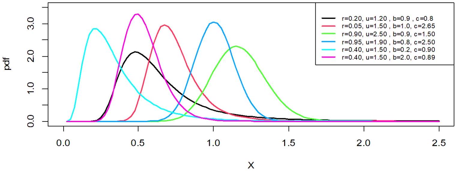
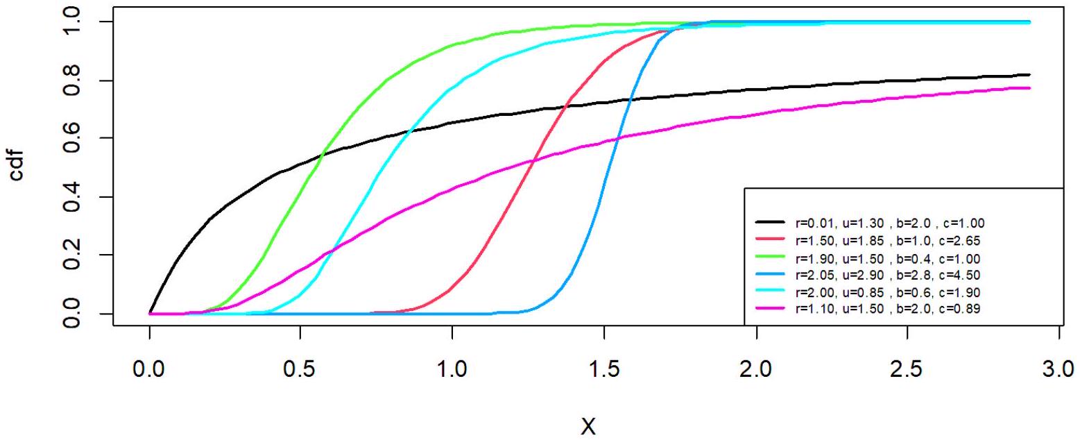
تقدم هذه الدراسة وتطبق نموذجًا إحصائيًا جديدًا يعرف بتوزيع وايبل العكسي الهجين (HWIW)، الذي يجمع بين خصائص توزيعي وايبل والعكسي وايبل لتوفير نموذج أكثر مرونة لتمثيل البيانات الواقعية، خاصة تلك التي تتميز باللامركزية أو القيم المتطرفة. تم اشتقاق الوظائف الأساسية للتوزيع، بالإضافة إلى اشتقاق مقاييس إحصائية أخرى مثل اللحظات، ودالة الكمية، والإنتروبيا. تم تقدير معلمات التوزيع باستخدام ثلاث طرق متميزة، وتم تقييم أدائها من خلال محاكاة مونت كارلو لتقييم أداء ودقة كل تقنية تقدير. تم استخدام النتائج لإظهار أكثر طرق التقدير دقة لعينات مختلفة. تم استخدام النموذج المقترح لاختبار مجموعتين عمليتين من البيانات؛ وأظهرت النتائج أن توزيع HWIW تفوق على ستة توزيعات IW منافسة من حيث مقاييس اختيار النموذج. تؤكد هذه النتائج كفاءة قدرة نموذج HWIW على التقاط هيكل مجموعات البيانات المعقدة وتفتح الطريق لاستخدامه في تطبيقات متعددة، بما في ذلك المجالات الطبية والصناعية والاجتماعية، مع إمكانية توسيعه ليشمل بيانات متعددة الأبعاد أو دمجه مع تقنيات الذكاء الاصطناعي.
1. المقدمة
لقد ساهمت في ظهور منهجية T-X، وهي واحدة من أبرز الطرق المستخدمة لتوليد توزيعات جديدة من خلال تحويل التوزيعات الأساسية باستخدام دوال تحويل مرنة. وقد أدت هذه المنهجية إلى ظهور عدة عائلات جديدة من التوزيعات [1]، مثل عائلة BIIIEE-X [2]، عائلة NOGEE-G [3]، عائلة WEE-X [2]، عائلة OLG [5]، عائلة NGOF-G [6]، عائلة EOIW-G [7]، عائلة GOM-G [8]، HOLGE [9]، و HOE-
2. توزيع وايبول الهجين العكسي (HWIW)
وظيفة البقاء المرتبطة بتوزيع HWIW تُعطى بالتعبير التالي [13] :
باتباع نفس النهج، يمكن أيضًا تبسيط PDF من خلال التوسع الرياضي، مما يؤدي إلى الصيغة التالية:
كـ
3. خصائص توزيع HWIW
3.1 دالة الكمية لتوزيع HWIW
افترض أن
لذلك
الآن، عُد إلى الوراء لإيجاد
قسمة كلا الجانبين على -ب يعطي:
تم تحديد تمثيل عددي لدالة الكوانتيل للنموذج المقترح في الجدول 1.
|
|
(
|
||||
| (0.7,1.3,0.4,0.2) | (0.6,1.5,1.4,1) | (0.5,1.1,0.9,1.1) | (1.2,1,0.8,1.2) | (0.7,1.9,0.7,0.5) | |
| 0.1 | 0.0218168 | 1.906395 | 1.062304 | 0.6697021 | 1.099829 |
| 0.2 | 0.1115255 | ٢.٦٢٠٩٣٠ | 1.532390 | 0.8610302 | 1.868169 |
| 0.3 | 0.3981566 | 3.348908 | 2.071615 | 1.0475163 | ٢.٧٦٥٠٩٤ |
| 0.4 | 1.2719911 | ٤.١٧٦٧٧٦ | 2.766355 | 1.2531876 | ٣.٨٩٠٤٠٠ |
| 0.5 | ٤.٠٤١٤٥٥٠ | 5.189129 | ٣.٧٤٤٧٥٦ | 1.4990069 | 5.381479 |
| 0.6 | 13.8737973 | 6.519626 | ٥.٢٦٧٠٤٧ | 1.8168022 | 7.483554 |
| 0.7 | 57.2273272 | 8.437554 | 7.985730 | 2.2706451 | 10.714995 |
| 0.8 | ٣٤٧.٧٥٩٦٩٦٥ | 11.637871 | 14.089895 | ٣.٠٢٩٦٣٠٥ | 16.449317 |
| 0.9 | ٥٧٤.١٨٩٠١٦٥ | 18.902468 | ٣٦.٧١٢٧٢١ | ٤.٨٠٥٢٣٧١ | 30.300980 |
3.2 دالة العزم لتوزيع HWIW
لـ
|
|
|
|
ج |
|
|
|
|
|
انحراف | التفرطح |
|
|
– |
|
1.1 | 1.596876 | ٤.٧٨٦٣٢٦ | ٣٧.٦١٦٩١ | ١٣٦٣.٢٥٦ | ٢.٢٣٦٣١٣ | ٣.٥٩٢٣٥٩ | ٥٩٫٥٠٧٦٦ |
| 1.2 | 1.50402 | ٣.٧٧٢٣٦٤ | 19.97024 | ٣٣٣.٨٢٠٥ | 1.510288 | 2.725605 | ٢٣.٤٥٧٧٢ | |||
| ج | 1.3 | 1.959321 | 5.865176 | 31.84193 | 157.4864 | ٢.٠٢٦٢٣٧ | ٢.٢٤١٧٠٢ | ٤.٥٧٨٠٥٤ | ||
| 1.4 | 1.844062 | ٤.٨٦٠٠٧١ | 20.81439 | 179.4392 | 1.459506 | 1.942673 | 7.596825 | |||
|
|
٨ | 1.5 | 2.012762 | ٤.٨٦٣٨٥ | 14.33673 | 52.54653 | 0.812639 | 1.336533 | ٢.٢٢١١٨ | |
| 1.6 | 1.916656 | ٤.٣١٠٣٩٤ | 11.52101 | ٣٧.١٦٤٦٦ | 0.636824 | 1.287405 | 2.000305 | |||
| 60 | 1.7 | 1.968528 | ٤.٤٦١٨١٦ | ١١.٧٦٧٤٨ | ٣٦.٥٦٤٧٨ | 0.586714 | 1.248579 | 1.836706 | ||
| 1.8 | 1.769355 | ٣.٥٤٨٣٨٤ | 8.136669 | 21.553 | 0.417767 | 1.217309 | 1.711774 |
3.3 دالة توليد اللحظات لتوزيع HWIW
3.4 دالة اللحظات غير المكتملة لتوزيع HWIW
3.5 الدالة المميزة لتوزيع HWIW
3.6 إنتروبيا ريني لتوزيع NMWIW
4. التقدير
4.1 تقدير الاحتمالية القصوى (MLE)
4.2 تقدير المربعات الصغرى
4.3 تقدير المربعات الصغرى الموزونة (WLSE)
5. المحاكاة
|
|
|||||
| ن | تأسس. | أس. بار. | MLE | لندن سكول أوف إيكونوميكس | WLSE |
| 50 | معنى |
|
0.66218994 | 0.7935073 | 0.7945322 |
|
|
0.94482752 | 0.90725405 | 0.87221447 | ||
|
|
0.8173529 | 0.9586352 | 0.9458078 | ||
|
|
1.6005334 | 1.3007755 | 1.3224457 | ||
| MSE |
|
0.34450955 | 0.3029998 | 0.3196053 | |
|
|
0.09171262 | 0.16296775 | 0.09943654 | ||
|
|
0.5872540 | 0.5312079 | 0.5426379 | ||
|
|
0.8883328 | 0.4236644 | 0.3828196 | ||
| جذر متوسط مربع الخطأ |
|
0.58694936 | 0.5504542 | 0.5653365 | |
|
|
0.30284092 | 0.40369264 | 0.31533560 | ||
|
|
0.7663250 | 0.7288401 | 0.7366396 | ||
|
|
0.9425141 | 0.6508951 | 0.6187241 | ||
| تحيز |
|
0.06218994 | 0.1935073 | 0.1945322 | |
|
|
0.04482752 | 0.00725405 | 0.02778553 | ||
|
|
0.1173529 | 0.2586352 | 0.02778553 | ||
|
|
0.4005334 | 0.1007755 | 0.1224457 | ||
| 100 | معنى |
|
0.64384318 | 0.7219438 | 0.7182429 |
|
|
0.94033751 | 0.87454167 | 0.87775399 | ||
|
|
0.76723431 | 0.8778392 | 0.8340620 | ||
|
|
1.4001384 | 1.3028549 | 1.27703038 | ||
| MSE |
|
0.23499950 | 0.2124502 | 0.1981540 | |
|
|
0.06256473 | 0.07460193 | 0.04674475 | ||
|
|
0.33109832 | 0.3405407 | 0.2714449 | ||
|
|
0.2971453 | 0.2258667 | 0.18424882 | ||
| جذر متوسط مربع الخطأ |
|
0.48476747 | 0.4609232 | 0.4451449 | |
|
|
0.25012943 | 0.27313355 | 0.21620533 | ||
|
|
0.57541144 | 0.5835586 | 0.5210037 | ||
|
|
0.5451103 | 0.4752543 | 0.42924215 | ||
| تحيز |
|
0.5451103 | 0.1219438 | 0.1182429 | |
|
|
0.04033751 | 0.02545833 | 0.02224601 | ||
|
|
0.06723431 | 0.1778392 | 0.1340620 | ||
|
|
0.2001384 | 0.1028549 | 0.07703038 |
| 150 | معنى |
|
0.609999358 | 0.7218282 | 0.64903158 |
|
|
0.95149716 | 0.87361891 | 0.91132615 | ||
|
|
0.72423747 | 0.8539909 | 0.75548383 | ||
|
|
1.3746361 | 1.27230291 | 0.75548383 | ||
| MSE |
|
0.180700778 | 0.2093021 | 0.16223096 | |
|
|
0.05561927 | 0.05271935 | 0.04119156 | ||
|
|
0.25410926 | 0.2817639 | 0.20157287 | ||
|
|
0.2018948 | 0.13858398 | 0.1762926 | ||
| جذر متوسط مربع الخطأ |
|
0.425089141 | 0.4574955 | 0.40277904 | |
|
|
0.23583739 | 0.22960694 | 0.20295704 | ||
|
|
0.50409251 | 0.5308143 | 0.44896867 | ||
|
|
0.4493271 | 0.37226869 | 0.4198721 | ||
| تحيز |
|
0.009999358 | 0.1218282 | 0.04903158 | |
|
|
0.05149716 | 0.02638109 | 0.01132615 | ||
|
|
0.02423747 | 0.1539909 | 0.05548383 | ||
|
|
0.1746361 | 0.07230291 | 0.1213862 | ||
| معنى |
|
0.62953303 | 0.67330833 | 0.62552888 | |
|
|
0.92401550 | 0.892643858 | 0.91648996 | ||
|
|
0.73728692 | 0.8049638 | 0.7284962 | ||
|
|
1.3183908 | 1.25742869 | 1.3022389 | ||
| MSE |
|
0.14542449 | 0.12782454 | 0.12441776 | |
|
|
0.03766835 | 0.043226750 | 0.03072519 | ||
|
|
0.18643346 | 0.2099843 | 0.1550041 | ||
|
|
0.1322101 | 0.11526679 | 0.1274526 |
| ٢٠٠ | جذر متوسط مربع الخطأ |
|
0.38134563 | 0.3636071 | 0.35272902 |
|
|
0.19408336 | 0.207910437 | 0.17528603 | ||
|
|
0.43177941 | 0.4582404 | 0.3937056 | ||
|
|
0.3636071 | 0.33950963 | 0.3570051 | ||
| تحيز |
|
0.02953303 | 0.07330833 | 0.02552888 | |
|
|
0.02401550 | 0.007356142 | 0.01648996 | ||
|
|
0.03728692 | 0.1049638 | 0.0284962 | ||
|
|
0.1183908 | 0.05742869 | 0.1022389 | ||
| ٢٥٠ | معنى |
|
0.605497333 | 0.67616917 | 0.608383893 |
|
|
0.93281004 | 0.88124099 | 0.92341073 | ||
|
|
0.706005227 | 0.79824836 | 0.71403583 | ||
|
|
1.30557693 | 1.26590402 | 1.29949605 | ||
| MSE |
|
0.109527538 | 0.12320369 | 0.108918047 | |
|
|
0.03389573 | 0.03761672 | 0.03328868 | ||
|
|
0.136416881 | 0.17672820 | 0.14360899 | ||
|
|
0.09854788 | 0.10182472 | 0.10257126 | ||
| جذر متوسط مربع الخطأ |
|
0.330949450 | 0.35100383 | 0.330027342 | |
|
|
0.18410793 | 0.19395029 | 0.18245186 | ||
|
|
0.369346559 | 0.42039054 | 0.37895777 | ||
|
|
0.31392336 | 0.31909986 | 0.32026748 | ||
| تحيز |
|
0.005497333 | 0.07616917 | 0.008383893 | |
|
|
0.03281004 | 0.01875901 | 0.02341073 | ||
|
|
0.006005227 | 0.09824836 | 0.01403583 | ||
|
|
0.10557693 | 0.06590402 | 0.09949605 |
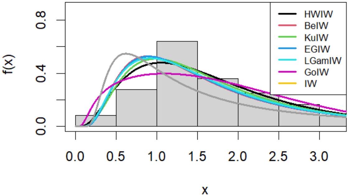
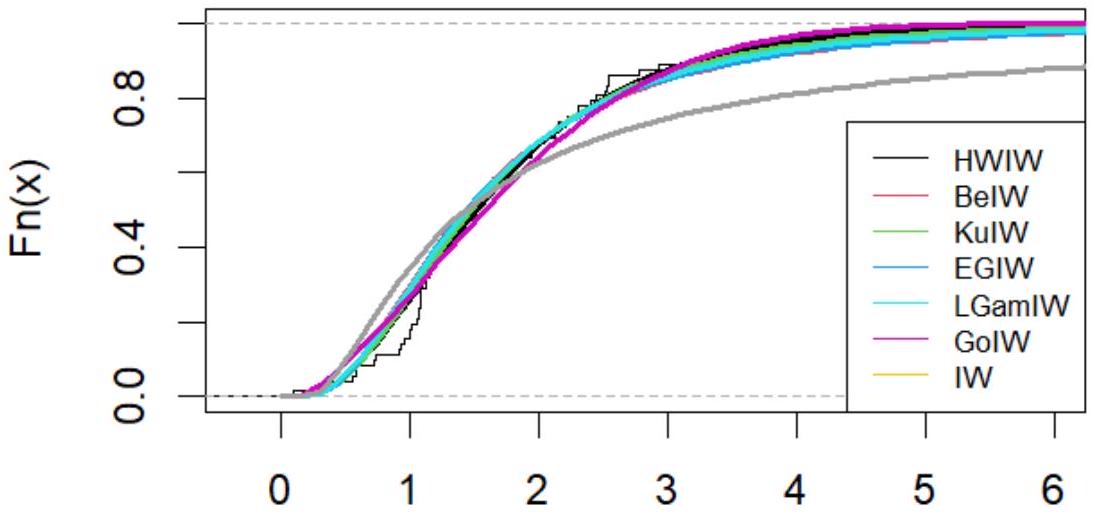
6. التطبيق
- بيتا مع توزيع وايبل العكسي الأساسي (BeIW)
- كوماراسوامي مع توزيع وايبول العكسي الأساسي (KuIW)
- الويبل المعكوس العام المعزز (EGIW)
- لوغ-جاما مع توزيع وايبول العكسي الأساسي (LGamIW)
- غومبيرتس مع وايبول عكسي أساسي (GoIW)
- ويبل العكسي (IW)
| منطقة | -لوج | إيه آي سي | CAIC | بيك | HQIC |
| HWIW | 95.88984 | 199.8247 | ٢٠٠.٤٢١٧ | ٢٠٨.٩٣١٣ | ٢٠٣.٤٥٠١ |
| كن | ١٠١.٢٩٦ | 210.6642 | 211.2612 | ٢١٩.٧٧٠٨ | ٢١٤.٢٨٩٥ |
| KuIW | 97.89873 | 203.7986 | 204.3956 | 212.9053 | ٢٠٧.٤٢٤ |
| إيجي و | 100.9368 | ٢٠٩.٨٨٢٦ | 210.4796 | 218.9893 | ٢١٣.٥٠٨ |
| LGamIW | 99.80569 | ٢٠٧.٦٢٤٧ | ٢٠٨.٢٢١٧ | 216.7314 | 211.2501 |
| GoIW | 97.17087 | ٢٠٢.٣٤١٨ | ٢٠٢.٩٣٨٨ | 211.4485 | 205.9672 |
| آي دبليو | ١١٨.١١٧٨ | ٢٤٠٫٢٣٥٦ | 240.4095 | 244.7889 | 242.0483 |
| منطقة | W | أ | K-S | قيمة p |
| HWIW | 0.0922143 | 0.6110752 | 0.1130676 | 0.316085 |
| كن | 0.1675262 | 1.155408 | 0.1438356 | 0.1016569 |
| KuIW | 0.1107239 | 0.7703783 | 0.11985 | 0.2522606 |
| إي جي آي دبليو | 0.1608632 | 1.111592 | 0.1402135 | 0.117882 |
| LGamIW | 21.91134 | ١٤١٫٢٥٨ | 0.9999952 |
|
| GoIW | 0.1616563 | 0.9825052 | 0.1283847 | 0.1861575 |
| آي دبليو | 0.5284354 | 3.310617 | 0.1991304 | 0.006625223 |
| منطقة |
|
|
|
|
| HWIW | 1.3782752 | 3.1107381 | 0.4686840 | 0.5414699 |
| كن | 0.9168564 | 5.9240884 | ٣.٠٠٧٤٠٥٨ | 0.7257823 |
| KuIW | 2.0448702 | 15.6432752 | 1.9116895 | 0.5584649 |
| إيجي و | 6.5028232 | 0.9572174 | ٣.٠٢١٥٦٧٣ | 0.7065691 |
| LGamIW | 0.6738629 | 7.9310308 | ٣.٩٧٦٧٦٩٠ | 0.7099198 |
| GoIW | 0.7349332 | ٣.٢٢٤٣٢٩٧ | 1.4417615 | 0.6936903 |
| آي دبليو | —- | —– | 1.061440 | 1.171994 |
| منطقة | -لوج | إيه آي سي | CAIC | بيك | HQIC |
| HWIW | ١٠٢.٥٨٩٧ | 213.1842 | ٢١٤.٠٧٣١ | ٢٢٠.٨٣٢٣ | 216.0967 |
| كن | ١٠٤.٧٦٢٢ | ٢١٧.٥٤٠٤ | 218.4292 | ٢٢٥.١٨٨٤ | 220.4528 |
| KuIW | ١٠٤.٤١٠٤ | 216.8386 | ٢١٧.٧٢٧٥ | 224.4867 | ٢١٩.٧٥١١ |
| إيجي و | ١٠٤.٧٦٧١ | ٢١٧.٥٤٣٨ | 218.4327 | ٢٢٥.١٩١٩ | ٢٢٠.٤٥٦٢ |
| LGamIW | ١٠٤.٤٦٥١ | ٢١٧.٠١٨٦ | ٢١٧.٩٠٧٥ | ٢٢٤.٦٦٦٧ | ٢١٩.٩٣١ |
| GoIW | ١٠٤.٥٨٧٣ | 217.1846 | 218.0735 | 224.8327 | ٢٢٠٫٠٩٧١ |
| آي دبليو | ١٠٦.٠٩٦٧ | 216.1933 | 216.4486 | 220.0174 | ٢١٧.٦٤٩٥ |
| منطقة | W | أ | K-S | قيمة p |
| HWIW | 0.1719594 | 1.063281 | 0.1379881 | 0.2711381 |
| كن | 0.2246938 | 1.384528 | 0.1585079 | 0.1453208 |
| KuIW | 0.2160847 | 1.333744 | 0.1558378 | 0.1584046 |
| إي جي آي دبليو | 0.224653 | 1.384445 | 0.1614739 | 0.1318197 |
| LGamIW | 17.95769 | 99.77021 | 0.9818669 |
|
| GoIW | 0.2123711 | 1.31562 | 0.1496055 | 0.1925845 |
| آي دبليو | 0.2575837 | 1.57173 | 0.16011 | 0.1378965 |
| منطقة |
|
|
|
|
| HWIW | 1.2975383 | 2.5187226 | 0.3953556 | 0.2346634 |
| كن | 1.2809056 | ٢.١٩٩٧٤٦٣ | 1.0261864 | 0.3948558 |
| KuIW | 1.3911669 | ٢.٧٤٠٧٦٣٦ | 1.0465352 | 0.3649795 |
| إيجي و | 2.1705086 | 1.0785869 | 1.1698675 | 0.4009732 |
| LGamIW | 1.2129747 | ٢.٩٤٧٢٠٤٩ | 1.3521062 | 0.3473045 |
| GoIW | 1.2129747 | ٢.٩٤٧٢٠٤٩ | 1.3521062 | 0.3473045 |
| آي دبليو | —- | —– | 0.6040943 | 0.5912884 |
7. الخاتمة
تتميز توزيع HWIW بقدرتها على التكيف مع البيانات غير المتماثلة والثقيلة الذيل، مما يجعلها مناسبة لتمثيل مجموعة واسعة من مجموعات البيانات الواقعية. كشفت نتائج محاكاة مونت كارلو أن طريقة WLSE كانت الأكثر دقة من حيث MSE و RMSE، خاصة بالنسبة للعينات الصغيرة والمتوسطة الحجم، بينما أظهرت طريقة MLE تحيزًا أقل واستقرارًا أكبر مع زيادة حجم العينة. بالمقابل، أدت طريقة LES أداءً ضعيفًا نسبيًا، مما يبرز أهمية اختيار طريقة التقدير المناسبة بناءً على حجم العينة وأهداف التحليل – WLES للدقة و MLE للاستقرار. يتمتع التوزيع المقترح بخصائص رياضية متقدمة، مثل مرونة دوال الكثافة والتوزيع، وسهولة اشتقاق اللحظات، ودالة الكمية، والإنتروبيا، مما يعزز موثوقيته كأداة تحليلية في الإحصاءات التطبيقية. نظرًا لتفوقه على التوزيعات الأخرى، يعد HWIW نموذجًا واعدًا يمكن توسيعه ليشمل البيانات متعددة الأبعاد أو دمجه مع تقنيات الذكاء الاصطناعي وتعلم الآلة لتحسين التنبؤات في البيئات غير المؤكدة. تفتح هذه النتائج آفاقًا جديدة لاستخدام توزيع HWIW في مجموعة واسعة من التطبيقات الواقعية، بما في ذلك المجالات الطبية والصناعية والاجتماعية، حيث تقدم النماذج التقليدية تحديات في تمثيل التباين والانحراف في البيانات الحقيقية.
مساهمات المؤلفين:
بيان توافر البيانات:
تعارض المصالح:
References
[2] Hussain, S., Hassan, M. U., Rashid, M. S., and Ahmed, R. (2023). Families of Extended Exponentiated Generalized Distributions and Applications of Medical Data Using Burr III Extended Exponentiated Weibull Distribution. Mathematics, 14(11), 3090.
[3] Odeyale, A. B., Gulumbe, S. U., Umar, U., and Aremu, K. O. (2023). New Odd Generalized Exponentiated Exponential-G Family of Distributions. UMYU Scientifica, 4(2), 56-64.
[4] Noori, N. A., Khalaf, A. A., and Khaleel, M. A. (2023). A New Generalized Family of Odd Lomax-G Distributions Properties and Applications. Advances in the Theory of Nonlinear Analysis and Its Application, 4(7), 1-16.
[5] Sadiq, I. A., Doguwa, S. I., Yahaya, A., and Garba, J. (2023). New Generalized Odd Fréchet-G (NGOF-G) Family of Distribution with Statistical Properties and Applications. UMYU Scientifica, 3(2), 100-107.
[6] Abdelall, Y. Y., Hassan, A. S., and Almetwally, E. M. (2024). A new extension of the odd inverse Weibull-G family of distributions: Bayesian and non-Bayesian estimation with engineering applications. Computational Journal of Mathematical and Statistical Sciences, 2(3), 359-388.
[7] Ishaq, A. I., Panitanarak, U., Alfred, A. A., Suleiman, A. A., and Daud, H. (2024). The Generalized Odd Maxwell-Kumaraswamy Distribution: Its Properties and Applications. Contemporary Mathematics, 1(1), 711-742.
[8] Noori, N. A., Abdullah, K. N., and Khaleel, M. A. (2025). Data Modelling and Analysis Using Odd Lomax Generalized Exponential Distribution: an Empirical Study and Simulation. Iraqi Statisticians Journal, 1(2), 146-162.
[9] Mahdi, G. A., Khaleel, M. A., Gemeay, A. M., Nagy, M., Mansi, A. H., Hossain, M. M., and Hussam, E. (2024). A new hybrid odd exponential-
[10] Noori, N. A., and Khaleel, M. A. (2024). Estimation and Some Statistical Properties of the hybrid Weibull Inverse Burr Type X Distribution with Application to Cancer Patient Data. Iraqi Statisticians Journal, 2(1), 8-29.
[11] Noori, N. A., Khalaf, A. A., and Khaleel, M. A. (2024). A new expansion of the Inverse Weibull Distribution: Properties with Applications. Iraqi Statisticians Journal, 1(1), 52-62.
[12] Noori, N. A. (2023). Exploring the Properties, Simulation, and Applications of the Odd Burr XII Gompertz Distribution. Advances in the Theory of Nonlinear Analysis and Its Application, 4(7), 60-75.
[13] Khalaf, A. A., Khaleel, M. A., and Noori, N. A. (2024). A new expansion of the Inverse Weibull Distribution: Properties with Applications. Iraqi Statisticians Journal, 1(1), 52-62.
[14] Alanaz, M. M., and Algamal, Z. Y. (2023). Neutrosophic exponentiated inverse Rayleigh distribution: Properties and Applications. International Journal of Neutrosophic Science, 21(4), 36-43.
[15] Khalaf, A. A., Ibrahim, M. Q., and Noori, N. A. (2024). [0,1] Truncated Exponentiated Exponential Burr type X Distribution with Applications. Iraqi Journal of Science, 65(8), 4428-4440.
[16] Gómez, H. J., Santoro, K. I., Chamorro, I. B., Venegas, O., Gallardo, D. I., and Gómez, H. W. (2023). A Family of Truncated Positive Distributions. Mathematics, 11(21), 4431.
[17] Muhammad, B., Mohsin, M., and Aslam, M. (2021). Weibull-exponential distribution and its application in monitoring industrial process. Mathematical Problems in Engineering, 2021(1), 1-13.
[18] Al Abbasi, J. N., Resen, I. A., Abdulwahab, A. M., Oguntunde, P. E., Al-Mofleh, H., and Khaleel, M. A. (2023). The right truncated Xgamma-G family of distributions: Statistical properties and applications. AIP Conference Proceedings, 2834(1), 1-15.
[19] Al-Habib, K. H., Khaleel, M. A., and Al-Mofleh, H. (2023). A new family of truncated Nadarajah-Haghighi-G properties with real data applications. Tikrit Journal of Administrative and Economic Sciences, 19(61), 2.
[20] Afify, A. Z., Yousof, H., and Nadarajah, S. (2017). The beta transmuted-H family for lifetime data. Statistics and its Interface, 10(3), 505-520.
[21] Bhatti, F. A., Hamedani, G. G., Korkmaz, M. C., Cordeiro, G. M., Yousof, H. M., and Ahmad, M. (2019). On Burr III Marshal Olkin family: development, properties, characterizations and applications. Journal of Statistical Distributions and Applications, 6(1), 1-21.
[22] Teamah, A.-E. A. M., Elbanna, A. A., and Gemeay, A. M. (2020). Frèchet-Weibull distribution with applications to earthquakes data sets. Pakistan Journal of Statistics, 36(2), 135-147.
[23] Abd El-latif, A. M., Almulhim, F. A., Noori, N. A., Khaleel, M. A., and Alsaedi, B. S. (2025). Properties with application to medical data for new inverse Rayleigh distribution utilizing neutrosophic logic. Journal of Radiation Research and Applied Sciences, 18(2), 101391.
[24] Abed, R. A., Khaleel, M. A., and Noori, N. A. (2025). Modified Weibull-Fréchet Distribution Properties with Application. Iraqi Statisticians Journal, 1(2), 195-216.
[25] Noori, N. A., Ahmed, D. D., and Khaleel, M. A. (2025). Odd Lomax Chen distribution: An Innovative Statistical Tool for Improving Real Data Modeling and Its Practical Applications. Tikrit Journal of Administrative and Economic Sciences, 21(Special Issue, Part 1), 1098-1126.
[26] Noori, N. A., Khaleel, M. A., and Salih, A. M. (2025). Some Expansions to The Weibull Distribution Families with Two Parameters: A Review. Babylonian Journal of Mathematics, 1(1), 61-87.
[27] Noori, N. A., Khaleel, M. A., Khalaf, S. A., and Dutta, S. (2025). Analytical Modeling of Expansion for Odd Lomax Generalized Exponential Distribution in Framework of Neutrosophic Logic: a Theoretical and Applied on Neutrosophic Data. Innovation in Statistics and Probability, 1(1), 47-59.
[28] Habib, K. H., Khaleel, M. A., Al-Mofleh, H., Oguntunde, P. E., and Adeyeye, S. J. (2024). Parameters Estimation for the [0, 1] Truncated Nadarajah Haghighi Rayleigh Distribution. Scientific African, 1(1), e02105.
[29] Khaoula, A., Seddik-Ameur, N., Abd El-Baset, A. A., and Khaleel, M. A. (2022). The Topp-Leone Extended Exponential Distribution: Estimation Methods and Applications. Pakistan Journal of Statistics and Operation Research, 18(4), 817-836
© 2025 by the authors. Disclaimer / Publisher’s Note: The views, opinions, and data presented in all published content are solely those of the individual authors and contributors. They do not necessarily reflect the positions of Sphinx Scientific Press (SSP) or its editorial team. SSP and the editors disclaim any responsibility for harm or damage to individuals or property that may result from the use of any information, methods, instructions, or products mentioned in the content.
DOI: https://doi.org/10.64389/mjs.2025.01112
Publication Date: 2025-07-12
Research article
Development and Applications of a New Hybrid Weibull-Inverse Weibull Distribution
ARTICLE INFO
Keywords:
Parameter estimation
Hybrid distributions
Monte-Carlo simulation
Real data analysis
Mathematics Subject Classification:
Important Dates:
Revised: 8 July 2025
Accepted: 10 July 2025
Online: 12 July 2025
Abstract
This study introduces and applies a novel statistical model known as the hybrid Weibull inverse Weibull (HWIW) distribution, which combines the characteristics of the Weibull and inverse Weibull distributions to provide a more flexible model for representing real-world data, especially those characterized by asymmetry or extreme values. The basic functions of the distribution were derived, along with other statistical measures such as moments, the quantile function, and entropy were also derived. The distribution parameters were estimated using three distinct approaches, and their performance was evaluated through a Monte Carlo simulation to assess the performance and precision of each estimation technique. The results were used to show the most accurate estimation method for different samples. The proposed model was utilized to test two practical datasets; the findings demonstrated that the HWIW distribution outperformed six competing IW distributions in terms of model selection metrics. These results confirm the efficiency of the HWIW model’s ability to capture the structure of complex datasets and open the way for its use in multiple applications, including medical, industrial, and social fields, with the potential to be expanded to include multidimensional data or integrated with artificial intelligence techniques.
1. Introduction
have contributed to the emergence of the T-X methodology, one of the most prominent methods used to generate new distribution by transforming basic distribution using flexible transformation functions. This methodology has resulted in the emergence of several new distribution families [1], such as BIIIEE-X family [2], NOGEE-G family [3], WEE-X Family[2], OLG family [5], NGOF-G Family [6], EOIW-G Family [7], GOM-G family [8], HOLGE [9], and HOE-
2. The hybrid Weibull inverse Weibull (HWIW) distribution
The survival function corresponding to the HWIW distribution is given by the following expression [13] :
Following the same approach, the PDF can also be simplified through mathematical expansion, leading to the following formula:
As
3. Properties for HWIW distribution
3.1 Quantile function for HWIW distribution
Assume that
So that
Now, substitute back to find
Dividing both sides by -b yields:
A numerical representation of our proposed model quantile function is determined in Table 1.
|
|
(
|
||||
| (0.7,1.3,0.4,0.2) | (0.6,1.5,1.4,1) | (0.5,1.1,0.9,1.1) | (1.2,1,0.8,1.2) | (0.7,1.9,0.7,0.5) | |
| 0.1 | 0.0218168 | 1.906395 | 1.062304 | 0.6697021 | 1.099829 |
| 0.2 | 0.1115255 | 2.620930 | 1.532390 | 0.8610302 | 1.868169 |
| 0.3 | 0.3981566 | 3.348908 | 2.071615 | 1.0475163 | 2.765094 |
| 0.4 | 1.2719911 | 4.176776 | 2.766355 | 1.2531876 | 3.890400 |
| 0.5 | 4.0414550 | 5.189129 | 3.744756 | 1.4990069 | 5.381479 |
| 0.6 | 13.8737973 | 6.519626 | 5.267047 | 1.8168022 | 7.483554 |
| 0.7 | 57.2273272 | 8.437554 | 7.985730 | 2.2706451 | 10.714995 |
| 0.8 | 347.7596965 | 11.637871 | 14.089895 | 3.0296305 | 16.449317 |
| 0.9 | 574.1890165 | 18.902468 | 36.712721 | 4.8052371 | 30.300980 |
3.2 Moment function for HWIW distribution
For
|
|
|
|
C |
|
|
|
|
|
skew | kurtosis |
|
|
– |
|
1.1 | 1.596876 | 4.786326 | 37.61691 | 1363.256 | 2.236313 | 3.592359 | 59.50766 |
| 1.2 | 1.50402 | 3.772364 | 19.97024 | 333.8205 | 1.510288 | 2.725605 | 23.45772 | |||
| g | 1.3 | 1.959321 | 5.865176 | 31.84193 | 157.4864 | 2.026237 | 2.241702 | 4.578054 | ||
| 1.4 | 1.844062 | 4.860071 | 20.81439 | 179.4392 | 1.459506 | 1.942673 | 7.596825 | |||
|
|
8 | 1.5 | 2.012762 | 4.86385 | 14.33673 | 52.54653 | 0.812639 | 1.336533 | 2.22118 | |
| 1.6 | 1.916656 | 4.310394 | 11.52101 | 37.16466 | 0.636824 | 1.287405 | 2.000305 | |||
| 60 | 1.7 | 1.968528 | 4.461816 | 11.76748 | 36.56478 | 0.586714 | 1.248579 | 1.836706 | ||
| 1.8 | 1.769355 | 3.548384 | 8.136669 | 21.553 | 0.417767 | 1.217309 | 1.711774 |
3.3 Moment Generating function for HWIW distribution
3.4 Incomplete Moments function for HWIW distribution
3.5 Characteristic function of HWIW distribution
3.6 Rényi entropy for NMWIW distribution
4. Estimation
4.1 Maximum likelihood estimation (MLE)
4.2 Least square estimation
4.3 Weighted Least square estimation (WLSE)
5. Simulation
|
|
|||||
| N | Est. | Ess. Par. | MLE | LSE | WLSE |
| 50 | Mean |
|
0.66218994 | 0.7935073 | 0.7945322 |
|
|
0.94482752 | 0.90725405 | 0.87221447 | ||
|
|
0.8173529 | 0.9586352 | 0.9458078 | ||
|
|
1.6005334 | 1.3007755 | 1.3224457 | ||
| MSE |
|
0.34450955 | 0.3029998 | 0.3196053 | |
|
|
0.09171262 | 0.16296775 | 0.09943654 | ||
|
|
0.5872540 | 0.5312079 | 0.5426379 | ||
|
|
0.8883328 | 0.4236644 | 0.3828196 | ||
| RMSE |
|
0.58694936 | 0.5504542 | 0.5653365 | |
|
|
0.30284092 | 0.40369264 | 0.31533560 | ||
|
|
0.7663250 | 0.7288401 | 0.7366396 | ||
|
|
0.9425141 | 0.6508951 | 0.6187241 | ||
| Bias |
|
0.06218994 | 0.1935073 | 0.1945322 | |
|
|
0.04482752 | 0.00725405 | 0.02778553 | ||
|
|
0.1173529 | 0.2586352 | 0.02778553 | ||
|
|
0.4005334 | 0.1007755 | 0.1224457 | ||
| 100 | Mean |
|
0.64384318 | 0.7219438 | 0.7182429 |
|
|
0.94033751 | 0.87454167 | 0.87775399 | ||
|
|
0.76723431 | 0.8778392 | 0.8340620 | ||
|
|
1.4001384 | 1.3028549 | 1.27703038 | ||
| MSE |
|
0.23499950 | 0.2124502 | 0.1981540 | |
|
|
0.06256473 | 0.07460193 | 0.04674475 | ||
|
|
0.33109832 | 0.3405407 | 0.2714449 | ||
|
|
0.2971453 | 0.2258667 | 0.18424882 | ||
| RMSE |
|
0.48476747 | 0.4609232 | 0.4451449 | |
|
|
0.25012943 | 0.27313355 | 0.21620533 | ||
|
|
0.57541144 | 0.5835586 | 0.5210037 | ||
|
|
0.5451103 | 0.4752543 | 0.42924215 | ||
| Bias |
|
0.5451103 | 0.1219438 | 0.1182429 | |
|
|
0.04033751 | 0.02545833 | 0.02224601 | ||
|
|
0.06723431 | 0.1778392 | 0.1340620 | ||
|
|
0.2001384 | 0.1028549 | 0.07703038 |
| 150 | Mean |
|
0.609999358 | 0.7218282 | 0.64903158 |
|
|
0.95149716 | 0.87361891 | 0.91132615 | ||
|
|
0.72423747 | 0.8539909 | 0.75548383 | ||
|
|
1.3746361 | 1.27230291 | 0.75548383 | ||
| MSE |
|
0.180700778 | 0.2093021 | 0.16223096 | |
|
|
0.05561927 | 0.05271935 | 0.04119156 | ||
|
|
0.25410926 | 0.2817639 | 0.20157287 | ||
|
|
0.2018948 | 0.13858398 | 0.1762926 | ||
| RMSE |
|
0.425089141 | 0.4574955 | 0.40277904 | |
|
|
0.23583739 | 0.22960694 | 0.20295704 | ||
|
|
0.50409251 | 0.5308143 | 0.44896867 | ||
|
|
0.4493271 | 0.37226869 | 0.4198721 | ||
| Bias |
|
0.009999358 | 0.1218282 | 0.04903158 | |
|
|
0.05149716 | 0.02638109 | 0.01132615 | ||
|
|
0.02423747 | 0.1539909 | 0.05548383 | ||
|
|
0.1746361 | 0.07230291 | 0.1213862 | ||
| Mean |
|
0.62953303 | 0.67330833 | 0.62552888 | |
|
|
0.92401550 | 0.892643858 | 0.91648996 | ||
|
|
0.73728692 | 0.8049638 | 0.7284962 | ||
|
|
1.3183908 | 1.25742869 | 1.3022389 | ||
| MSE |
|
0.14542449 | 0.12782454 | 0.12441776 | |
|
|
0.03766835 | 0.043226750 | 0.03072519 | ||
|
|
0.18643346 | 0.2099843 | 0.1550041 | ||
|
|
0.1322101 | 0.11526679 | 0.1274526 |
| 200 | RMSE |
|
0.38134563 | 0.3636071 | 0.35272902 |
|
|
0.19408336 | 0.207910437 | 0.17528603 | ||
|
|
0.43177941 | 0.4582404 | 0.3937056 | ||
|
|
0.3636071 | 0.33950963 | 0.3570051 | ||
| Bias |
|
0.02953303 | 0.07330833 | 0.02552888 | |
|
|
0.02401550 | 0.007356142 | 0.01648996 | ||
|
|
0.03728692 | 0.1049638 | 0.0284962 | ||
|
|
0.1183908 | 0.05742869 | 0.1022389 | ||
| 250 | Mean |
|
0.605497333 | 0.67616917 | 0.608383893 |
|
|
0.93281004 | 0.88124099 | 0.92341073 | ||
|
|
0.706005227 | 0.79824836 | 0.71403583 | ||
|
|
1.30557693 | 1.26590402 | 1.29949605 | ||
| MSE |
|
0.109527538 | 0.12320369 | 0.108918047 | |
|
|
0.03389573 | 0.03761672 | 0.03328868 | ||
|
|
0.136416881 | 0.17672820 | 0.14360899 | ||
|
|
0.09854788 | 0.10182472 | 0.10257126 | ||
| RMSE |
|
0.330949450 | 0.35100383 | 0.330027342 | |
|
|
0.18410793 | 0.19395029 | 0.18245186 | ||
|
|
0.369346559 | 0.42039054 | 0.37895777 | ||
|
|
0.31392336 | 0.31909986 | 0.32026748 | ||
| Bias |
|
0.005497333 | 0.07616917 | 0.008383893 | |
|
|
0.03281004 | 0.01875901 | 0.02341073 | ||
|
|
0.006005227 | 0.09824836 | 0.01403583 | ||
|
|
0.10557693 | 0.06590402 | 0.09949605 |
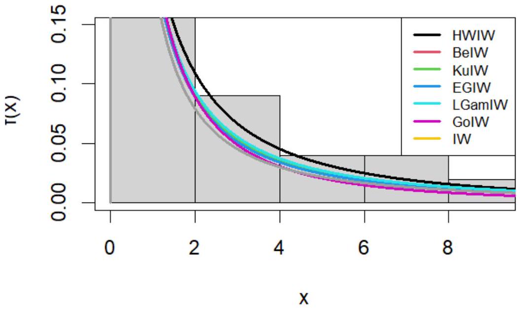
6. Application
- Beta with baseline inverse Weibull (BeIW)
- Kumaraswamy with baseline inverse Weibull (KuIW)
- Exponeted generalized with baseline inverse Weibull (EGIW)
- Log-Gamma with baseline inverse Weibull (LGamIW)
- Gompertz with baseline inverse Weibull (GoIW)
- Inverse Wiebull (IW)
| Dist. | -log | AIC | CAIC | BIC | HQIC |
| HWIW | 95.88984 | 199.8247 | 200.4217 | 208.9313 | 203.4501 |
| BeIW | 101.296 | 210.6642 | 211.2612 | 219.7708 | 214.2895 |
| KuIW | 97.89873 | 203.7986 | 204.3956 | 212.9053 | 207.424 |
| EGIW | 100.9368 | 209.8826 | 210.4796 | 218.9893 | 213.508 |
| LGamIW | 99.80569 | 207.6247 | 208.2217 | 216.7314 | 211.2501 |
| GoIW | 97.17087 | 202.3418 | 202.9388 | 211.4485 | 205.9672 |
| IW | 118.1178 | 240.2356 | 240.4095 | 244.7889 | 242.0483 |
| Dist. | W | A | K-S | p-value |
| HWIW | 0.0922143 | 0.6110752 | 0.1130676 | 0.316085 |
| BeIW | 0.1675262 | 1.155408 | 0.1438356 | 0.1016569 |
| KuIW | 0.1107239 | 0.7703783 | 0.11985 | 0.2522606 |
| EGIW | 0.1608632 | 1.111592 | 0.1402135 | 0.117882 |
| LGamIW | 21.91134 | 141.258 | 0.9999952 |
|
| GoIW | 0.1616563 | 0.9825052 | 0.1283847 | 0.1861575 |
| IW | 0.5284354 | 3.310617 | 0.1991304 | 0.006625223 |
| Dist. |
|
|
|
|
| HWIW | 1.3782752 | 3.1107381 | 0.4686840 | 0.5414699 |
| BeIW | 0.9168564 | 5.9240884 | 3.0074058 | 0.7257823 |
| KuIW | 2.0448702 | 15.6432752 | 1.9116895 | 0.5584649 |
| EGIW | 6.5028232 | 0.9572174 | 3.0215673 | 0.7065691 |
| LGamIW | 0.6738629 | 7.9310308 | 3.9767690 | 0.7099198 |
| GoIW | 0.7349332 | 3.2243297 | 1.4417615 | 0.6936903 |
| IW | —- | —– | 1.061440 | 1.171994 |
| Dist. | -log | AIC | CAIC | BIC | HQIC |
| HWIW | 102.5897 | 213.1842 | 214.0731 | 220.8323 | 216.0967 |
| BeIW | 104.7622 | 217.5404 | 218.4292 | 225.1884 | 220.4528 |
| KuIW | 104.4104 | 216.8386 | 217.7275 | 224.4867 | 219.7511 |
| EGIW | 104.7671 | 217.5438 | 218.4327 | 225.1919 | 220.4562 |
| LGamIW | 104.4651 | 217.0186 | 217.9075 | 224.6667 | 219.931 |
| GoIW | 104.5873 | 217.1846 | 218.0735 | 224.8327 | 220.0971 |
| IW | 106.0967 | 216.1933 | 216.4486 | 220.0174 | 217.6495 |
| Dist. | W | A | K-S | p-value |
| HWIW | 0.1719594 | 1.063281 | 0.1379881 | 0.2711381 |
| BeIW | 0.2246938 | 1.384528 | 0.1585079 | 0.1453208 |
| KuIW | 0.2160847 | 1.333744 | 0.1558378 | 0.1584046 |
| EGIW | 0.224653 | 1.384445 | 0.1614739 | 0.1318197 |
| LGamIW | 17.95769 | 99.77021 | 0.9818669 |
|
| GoIW | 0.2123711 | 1.31562 | 0.1496055 | 0.1925845 |
| IW | 0.2575837 | 1.57173 | 0.16011 | 0.1378965 |
| Dist. |
|
|
|
|
| HWIW | 1.2975383 | 2.5187226 | 0.3953556 | 0.2346634 |
| BeIW | 1.2809056 | 2.1997463 | 1.0261864 | 0.3948558 |
| KuIW | 1.3911669 | 2.7407636 | 1.0465352 | 0.3649795 |
| EGIW | 2.1705086 | 1.0785869 | 1.1698675 | 0.4009732 |
| LGamIW | 1.2129747 | 2.9472049 | 1.3521062 | 0.3473045 |
| GoIW | 1.2129747 | 2.9472049 | 1.3521062 | 0.3473045 |
| IW | —- | —– | 0.6040943 | 0.5912884 |
7. Conclusion
the HWIW distribution’s adaptability to asymmetric and heavy-tailed data, making it well-suited for representing a wide range of realworld datasets. Monte-Carlo simulation results revealed that the WLSE method was the most accurate in terms of MSE and RMSE, particularly for small and medium-size samples, while the MLE method exhibited lower bias and greater stability as sample size increased. In contrast, the LES method performed relatively poorly, underscoring the importance of selecting the appropriate estimation method based on sample size and analysis goals-WLES for accuracy and MLE for stable. The proposed distribution possesses advanced mathematical properties, such as the flexibility of density and distribution functions, and the ease of deriving moments, quantile function, and entropy, enhancing its reliability as an analytical tool in applied statistics. Given its superiority over other distributions, the HWIW is a promising model that can be extended to multidimensional data or combined with artificial intelligence and machine learning techniques to improve predictions in uncertain environments. These results open new avenues for employing the HWIW distribution in a wide range of real-world applications, including medical, industrial, and social fields, where traditional models present challenges in representing variance and skewness in real data.
Authors’ Contributions:
Data Availability Statement:
Conflicts of Interest:
References
[2] Hussain, S., Hassan, M. U., Rashid, M. S., and Ahmed, R. (2023). Families of Extended Exponentiated Generalized Distributions and Applications of Medical Data Using Burr III Extended Exponentiated Weibull Distribution. Mathematics, 14(11), 3090.
[3] Odeyale, A. B., Gulumbe, S. U., Umar, U., and Aremu, K. O. (2023). New Odd Generalized Exponentiated Exponential-G Family of Distributions. UMYU Scientifica, 4(2), 56-64.
[4] Noori, N. A., Khalaf, A. A., and Khaleel, M. A. (2023). A New Generalized Family of Odd Lomax-G Distributions Properties and Applications. Advances in the Theory of Nonlinear Analysis and Its Application, 4(7), 1-16.
[5] Sadiq, I. A., Doguwa, S. I., Yahaya, A., and Garba, J. (2023). New Generalized Odd Fréchet-G (NGOF-G) Family of Distribution with Statistical Properties and Applications. UMYU Scientifica, 3(2), 100-107.
[6] Abdelall, Y. Y., Hassan, A. S., and Almetwally, E. M. (2024). A new extension of the odd inverse Weibull-G family of distributions: Bayesian and non-Bayesian estimation with engineering applications. Computational Journal of Mathematical and Statistical Sciences, 2(3), 359-388.
[7] Ishaq, A. I., Panitanarak, U., Alfred, A. A., Suleiman, A. A., and Daud, H. (2024). The Generalized Odd Maxwell-Kumaraswamy Distribution: Its Properties and Applications. Contemporary Mathematics, 1(1), 711-742.
[8] Noori, N. A., Abdullah, K. N., and Khaleel, M. A. (2025). Data Modelling and Analysis Using Odd Lomax Generalized Exponential Distribution: an Empirical Study and Simulation. Iraqi Statisticians Journal, 1(2), 146-162.
[9] Mahdi, G. A., Khaleel, M. A., Gemeay, A. M., Nagy, M., Mansi, A. H., Hossain, M. M., and Hussam, E. (2024). A new hybrid odd exponential-
[10] Noori, N. A., and Khaleel, M. A. (2024). Estimation and Some Statistical Properties of the hybrid Weibull Inverse Burr Type X Distribution with Application to Cancer Patient Data. Iraqi Statisticians Journal, 2(1), 8-29.
[11] Noori, N. A., Khalaf, A. A., and Khaleel, M. A. (2024). A new expansion of the Inverse Weibull Distribution: Properties with Applications. Iraqi Statisticians Journal, 1(1), 52-62.
[12] Noori, N. A. (2023). Exploring the Properties, Simulation, and Applications of the Odd Burr XII Gompertz Distribution. Advances in the Theory of Nonlinear Analysis and Its Application, 4(7), 60-75.
[13] Khalaf, A. A., Khaleel, M. A., and Noori, N. A. (2024). A new expansion of the Inverse Weibull Distribution: Properties with Applications. Iraqi Statisticians Journal, 1(1), 52-62.
[14] Alanaz, M. M., and Algamal, Z. Y. (2023). Neutrosophic exponentiated inverse Rayleigh distribution: Properties and Applications. International Journal of Neutrosophic Science, 21(4), 36-43.
[15] Khalaf, A. A., Ibrahim, M. Q., and Noori, N. A. (2024). [0,1] Truncated Exponentiated Exponential Burr type X Distribution with Applications. Iraqi Journal of Science, 65(8), 4428-4440.
[16] Gómez, H. J., Santoro, K. I., Chamorro, I. B., Venegas, O., Gallardo, D. I., and Gómez, H. W. (2023). A Family of Truncated Positive Distributions. Mathematics, 11(21), 4431.
[17] Muhammad, B., Mohsin, M., and Aslam, M. (2021). Weibull-exponential distribution and its application in monitoring industrial process. Mathematical Problems in Engineering, 2021(1), 1-13.
[18] Al Abbasi, J. N., Resen, I. A., Abdulwahab, A. M., Oguntunde, P. E., Al-Mofleh, H., and Khaleel, M. A. (2023). The right truncated Xgamma-G family of distributions: Statistical properties and applications. AIP Conference Proceedings, 2834(1), 1-15.
[19] Al-Habib, K. H., Khaleel, M. A., and Al-Mofleh, H. (2023). A new family of truncated Nadarajah-Haghighi-G properties with real data applications. Tikrit Journal of Administrative and Economic Sciences, 19(61), 2.
[20] Afify, A. Z., Yousof, H., and Nadarajah, S. (2017). The beta transmuted-H family for lifetime data. Statistics and its Interface, 10(3), 505-520.
[21] Bhatti, F. A., Hamedani, G. G., Korkmaz, M. C., Cordeiro, G. M., Yousof, H. M., and Ahmad, M. (2019). On Burr III Marshal Olkin family: development, properties, characterizations and applications. Journal of Statistical Distributions and Applications, 6(1), 1-21.
[22] Teamah, A.-E. A. M., Elbanna, A. A., and Gemeay, A. M. (2020). Frèchet-Weibull distribution with applications to earthquakes data sets. Pakistan Journal of Statistics, 36(2), 135-147.
[23] Abd El-latif, A. M., Almulhim, F. A., Noori, N. A., Khaleel, M. A., and Alsaedi, B. S. (2025). Properties with application to medical data for new inverse Rayleigh distribution utilizing neutrosophic logic. Journal of Radiation Research and Applied Sciences, 18(2), 101391.
[24] Abed, R. A., Khaleel, M. A., and Noori, N. A. (2025). Modified Weibull-Fréchet Distribution Properties with Application. Iraqi Statisticians Journal, 1(2), 195-216.
[25] Noori, N. A., Ahmed, D. D., and Khaleel, M. A. (2025). Odd Lomax Chen distribution: An Innovative Statistical Tool for Improving Real Data Modeling and Its Practical Applications. Tikrit Journal of Administrative and Economic Sciences, 21(Special Issue, Part 1), 1098-1126.
[26] Noori, N. A., Khaleel, M. A., and Salih, A. M. (2025). Some Expansions to The Weibull Distribution Families with Two Parameters: A Review. Babylonian Journal of Mathematics, 1(1), 61-87.
[27] Noori, N. A., Khaleel, M. A., Khalaf, S. A., and Dutta, S. (2025). Analytical Modeling of Expansion for Odd Lomax Generalized Exponential Distribution in Framework of Neutrosophic Logic: a Theoretical and Applied on Neutrosophic Data. Innovation in Statistics and Probability, 1(1), 47-59.
[28] Habib, K. H., Khaleel, M. A., Al-Mofleh, H., Oguntunde, P. E., and Adeyeye, S. J. (2024). Parameters Estimation for the [0, 1] Truncated Nadarajah Haghighi Rayleigh Distribution. Scientific African, 1(1), e02105.
[29] Khaoula, A., Seddik-Ameur, N., Abd El-Baset, A. A., and Khaleel, M. A. (2022). The Topp-Leone Extended Exponential Distribution: Estimation Methods and Applications. Pakistan Journal of Statistics and Operation Research, 18(4), 817-836
© 2025 by the authors. Disclaimer / Publisher’s Note: The views, opinions, and data presented in all published content are solely those of the individual authors and contributors. They do not necessarily reflect the positions of Sphinx Scientific Press (SSP) or its editorial team. SSP and the editors disclaim any responsibility for harm or damage to individuals or property that may result from the use of any information, methods, instructions, or products mentioned in the content.