DOI: https://doi.org/10.18637/jss.v112.i01
تاريخ النشر: 2025-01-01
توافق بشكل مقتصد مع تأثيرات عشوائية متعددة المتغيرات الكبيرة في glmmTMB
الملخص
آثار عشوائية متعددة المتغيرات مع مصفوفات التباين-التغاير غير الهيكلية ذات الأبعاد الكبيرة،
1. المقدمة
R> glmer(abundance ~ Zone + Year + (Species + 0 | ID), family = "poisson",
+ data = windfarm)
R> glmmTMB(abundance ~ Zone + Year + (Species + 0 | ID), family = "poisson",
+ data = windfarm)
إحدى الطرق الشائعة للتعامل مع الأبعاد العالية هي استخدام نهج منخفض الرتبة، من خلال إجراء افتراضات مبسطة تقلل من أبعاد المشكلة إلى
تم استخدام نماذج GLVM بشكل متكرر في علم البيئة والعلوم الاجتماعية، وكانت الأمثلة المبكرة نماذج لوجود أو غياب أنواع الأسماك (Walker و Jackson 2011) ونماذج لاختيار الأحزاب المتعددة وتصنيفات البيانات (Skrondal و Rabe-Hesketh 2003). يمكن أن تكون نماذج GLVM صعبة من الناحية التقنية، ولكن هناك عدد من الحلول البرمجية المخصصة. تستخدم حزمة gllamm (Rabe-Hesketh و Skrondal و Pickles 2004) في Stata (StataCorp 2023) تكامل غاوسي التكيف لإزالة المتغيرات الكامنة. استخدمت البرمجيات المبكرة المكتوبة بلغة R، مع وضع علماء البيئة في الاعتبار، سلسلة ماركوف بايزي (Hui 2016؛ Ovaskainen وآخرون 2017). يمكن الحصول على ملاءمات أسرع بكثير باستخدام تقريب لابلاس (Huber و Ronchetti و Victoria-Feser 2004؛ Niku و Warton و Hui و Taskinen 2017) أو تقريب تبايني (Hui و Warton و Ormerod و Haapaniemi و Taskinen 2017) لاحتمالية الهامش، كما هو مطبق في حزمة R gllvm (Niku وآخرون 2019). تم كتابة هذه الأدوات مع نموذج معين في الاعتبار، حيث يتم استخدام تقاطع عشوائي متعدد المتغيرات لفرض الارتباط عبر العديد من الاستجابات، وتستخدم التأثيرات الثابتة لربط المتنبئ الخطي بالمتغيرات المقاسة، على الرغم من وجود بعض التمديدات لتخفيف هذا القيد بطرق مختلفة (Van der Veen و Hui و Hovstad و Solbu و O’Hara 2021؛ Niku و Hui و Taskinen و Warton 2021). ومع ذلك، فإن هذه البرمجيات غير قادرة على التعامل مع مجموعة من تصاميم العينة الشائعة. مثال تم النظر فيه في القسم 3.2 هو عندما يكون التأثير العشوائي المتعدد المتغيرات له متغيرات قد تختلف عبر المجموعات وداخلها.
في هذه الورقة، نضيف وظيفة الرتبة المنخفضة إلى حزمة glmmTMB (بروكس وآخرون 2017) لنماذج التأثيرات المختلطة المرنة التي يمكن أن تشمل مصطلحات تحليل العوامل، للبيانات المتعددة المتغيرات.
آثار عشوائية ذات أبعاد كبيرة. حزمة glmmTMB، المتاحة من شبكة أرشيف R الشاملة (CRAN) فيhttps://CRAN.R-project.org/package=glmmTMBتم بناءه كامتداد لـ lme4 (Bates et al. 2014)، والذي يُستخدم على نطاق واسع في العلوم التطبيقية لمشاكل تتعلق بمجموعة من تصاميم الدراسة، بما في ذلك التصاميم متعددة المستويات وتصاميم القياسات المتكررة. يستخدم حزمة glmmTMB واجهة مشابهة لـ lme4 ولكنها تستفيد من التمايز التلقائي لتقدير أسرع لنماذج التأثيرات المختلطة (Brooks et al. 2017). من خلال إضافة وظيفة تقليل الرتبة إلى glmmTMB، نثري فئة النماذج المختلطة التي يمكن تركيبها لتشمل تأثيرات عشوائية متعددة المتغيرات بأبعاد أكبر بكثير مما كان ممكنًا سابقًا، بحيث يمكننا الآن تركيب تأثيرات عشوائية بأبعاد تصل إلى المئات، أو ربما الآلاف. تشمل هذه الفئة الجديدة من النماذج، على سبيل المثال، GLVMs مع وظيفة لأي من تصاميم الدراسة التي يمكن تحليلها باستخدام lme4، بما في ذلك التصاميم متعددة المستويات أو تصاميم القياسات المتكررة.
يوفر القسم 2 نظرة عامة على نموذج الانحدار الخطي المختلط العام، والامتدادات التحليلية للعوامل للتعامل مع التأثيرات العشوائية المتعددة الأبعاد ذات الأبعاد العالية، ونهج التقدير المستخدم في glmmTMB لتناسب مثل هذه النماذج. نصف استخدام glmmTMB لتناسب التأثيرات العشوائية المتعددة الأبعاد ذات الرتبة المخفضة. نقوم بتحليل مجموعتين مختلفتين من البيانات، من علم البيئة والعلوم الاجتماعية، في القسم 3. يختتم القسم 4 الورقة.
2. الطرق
2.1. النماذج
مع عدد المعلمات في
يتضمن نهج المرتبة المخفضة لتناسب تأثير عشوائي متعدد المتغيرات التعبير عنه كدالة خطية لـ
بالنظر إلى هذه التعريفات، فإن التأثير العشوائي المتعدد المتغيرات موزع كـ
2.2. التقدير
نركز على تقريب لابلاس لاحتمالية الهامش، والتي تُستخدم على نطاق واسع لنماذج التأثيرات المختلطة العامة (GLMMs) (راودنبوش، يانغ، ويوسف 2000) وكذلك لنماذج التأثيرات العامة المتغيرة (GLVMs) (هوبر وآخرون 2004؛ نيكو وآخرون 2017). من خلال كتابة المعادلة 3 بالشكل
يمكن كتابته كـ
في glmmTMB نقوم بتعظيم تقريب لابلاس للاحتمالية اللوغاريتمية الهامشية المستمدة من حزمة Template Model Builder (TMB) (كريستنسن، نيلسن، بيرغ، سكاوغ، وبل 2015) في R (أو بشكل أكثر دقة، تقليل اللوغاريتم السالب للاحتمالية). يقوم TMB بتقييم تقريب لابلاس ومشتقاته باستخدام التمايز التلقائي. يمكن استخدام أي طريقة تحسين تعتمد على التدرج متاحة في R للقيام بالتعظيم، وبشكل افتراضي يستخدم glmmTMB nlminb(). ثم يستخدم TMB طريقة دلتا المعممة لحساب الانحرافات المعيارية الهامشية للتأثيرات الثابتة والعشوائية (كاس وستيفي 1989).
2.3. واجهة البرمجيات
rr(x | المجموعة، 2)
لذا على سبيل المثال، لنموذج متوسط الاستجابة (y) كدالة لـ x ولتترك معاملات x تتغير عشوائيًا بين المجموعات كدالة لاثنين من المتغيرات الكامنة، تكون الصيغة هي
العدد الصحيح غير السالب بعد الفاصلة في المعادلة يحدد عدد المتغيرات الكامنة، أو الرتبة، لمصفوفة التباين-التغاير للتأثيرات العشوائية المتعددة، والتي تكون افتراضيًا
تتمثل إحدى المشكلات في ملاءمة نموذج تحليل العوامل في أن دالة الاحتمالية غالبًا ما تكون متعددة القمم، مما قد يؤدي إلى التقارب نحو حد أقصى محلي. للتغلب على ذلك، نقوم بتضمين طريقة مدفوعة بالبيانات استنادًا إلى عمل نيكو وآخرين (2019) لتهيئة القيم للمعلمات بحيث يبدأ خوارزمية التعظيم بالقرب من الحد الأقصى العالمي. الإعداد الافتراضي في glmmTMB يحدد قيم المعلمات على أنها صفر، أو واحد للمعلمات ذات التأثير الثابت لبعض دوال الربط. للتحكم في الخوارزمية المستخدمة لتهيئة المعلمات، يتم تحديد وسيط start_method، كقائمة تحتوي على مكونات method وانحراف التذبذبتمت إضافته إلى
glmmTMBControl(). تعيين الطريقة = “res” يناسب نموذج خطي عام (GLM) للبيانات للحصول على تقديرات المعلمات الثابتة، والتي تُستخدم بعد ذلك كقيم ابتدائية للمعلمات الثابتة. من النموذج الملائم، يتم حساب المتبقيات للنماذج باستخدام عائلات بواسون، ثنائية الحد السلبية، وثنائية الحد باستخدام الطريقة التي اقترحها دان وسميث (1996)، بينما تُستخدم الدالة الداخلية dev.residuals للعائلات الأخرى. قيم ابتدائية للمتغيرات الكامنة،
تظهر المزيد من الأمثلة على تنفيذ هيكل rr في القسم 3. يمكن العثور على معلومات حول هيكل التباين والتغاير ذو الرتبة المنخفضة والهياكل الأخرى المتاحة في glmmTMB في الكتيب (“covstruct”، الحزمة = “glmmTMB”).
3. التطبيق
3.1. بيانات مزرعة الرياح
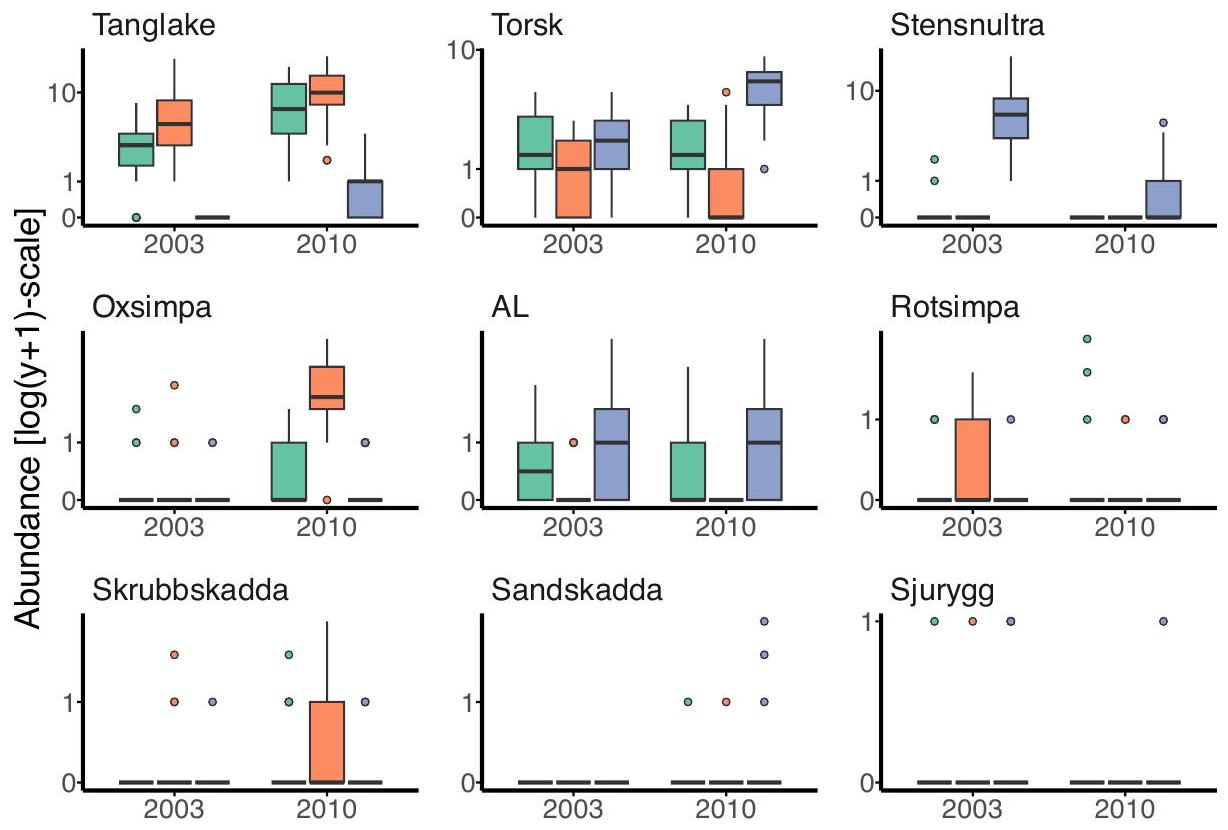
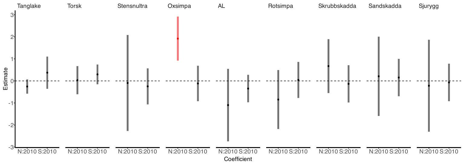
تتطلب التأثيرات العشوائية متعددة المتغيرات حساب الارتباط في استجابات الأنواع داخل عينة – نتوقع وجود ارتباط عبر الأنواع بسبب التفاعلات بين الأنواع، أو الاستجابة لظروف بيئية غير مرصودة (Warton et al. 2015) ونرغب في أن نكون قادرين على تقدير الارتباطات الإيجابية أو السلبية. ليس لدينا أي هيكل مسبق لهذا الارتباط، ولتسع أنواع سنحتاج إلى 45 معلمة لتقدير مصفوفة التباين-التغاير بين الأنواع. وبالتالي، نتوقع عدم استقرار كبير في الملاءمة، خاصة بالنسبة لمصطلحات الارتباط التي تتضمن الأنواع النادرة. بالمقارنة، ستتطلب بنية التغاير ذات الرتبة المخفضة من الرتبة الثانية 17 معلمة فقط.
نحن نضع نماذج للوفرة،
R> glmmTMB(abundance ~ Zone * Year + diag(Zone * Year | Species) +
+ (1 | Station) + rr(Species + 0 | ID, 2), family = "poisson",
+ control = glmmTMBControl(start_method = list(method = "res")),
+ data = windfarm)
glmmTMB.
| نموذج شرطي: | ||||||||||
| المجموعات | الاسم | الانحراف المعياري | الارتباط | |||||||
| المعرف | الأنواعTanglake | 0.4741 | ||||||||
| الأنواعTorsk | 0.1618 | 0.40 | ||||||||
| الأنواعStensnultra | 0.6963 | 0.36 | 1.00 | |||||||
| الأنواعOxsimpa | 0.2092 | -1.00 | -0.34 | -0.29 | ||||||
| الأنواعAL | 0.5502 | -0.85 | 0.13 | 0.18 | 0.89 | |||||
| الأنواعRotsimpa | 0.8684 | 0.24 | 0.99 | 0.99 | -0.17 | 0.30 | ||||
| الأنواعSkrubbskadda | 0.6541 | 0.43 | 1.00 | 1.00 | -0.36 | 0.10 | 0.98 | |||
| الأنواعSandskadda | 1.6886 | 0.39 | 1.00 | 1.00 | -0.32 | 0.14 | 0.99 | 1.00 | ||
| الأنواعSjurygg | 0.6395 | 0.52 | 0.99 | 0.98 | -0.46 | 0.00 | 0.95 | 0.99 | 0.99 | |
3.2. بيانات PIRLS
نقترح أن الطلاب من المدارس ذات الوضع الاقتصادي المتدني (Eco_disad) الذين لديهم مكتبة تحتوي على المزيد من الكتب (Size_lib) لديهم درجات محو أمية أعلى من الطلاب من مدرسة بلا مكتبة، لكن الفرق في درجات محو الأمية سيكون أقل عندما يكون الطلاب من مدارس ذات خلفية اقتصادية أعلى، أي أن هناك تفاعل بين المتغيرين المدرسيين. علاوة على ذلك، نود أن نعرف كيف سيتغير التأثير التفاعلي لهذه المتغيرات على مستوى المدرسة حسب البلد، ومن ثم نريد ملاءمة نموذج منحدرات عشوائية، مع تأثيرات مختلفة لـ Eco_disad:Size_lib لكل بلد. كلا من Eco_disad و Size_lib هما متغيرات فئوية بأربعة مستويات، وبالتالي نحتاج إلى 15 معلمة لوصف تأثيرهما المشترك و15 تأثير عشوائي ذو أبعاد في النموذج. تقدير مصفوفة التباين-التغاير غير الهيكلية
نعتبر النموذج لدرجة محو الأمية،
يمكن ملاءمة هذا النموذج في glmmTMB باستخدام الأمر التالي:
R> glmmTMB(Overall ~ Size_lib * Eco_disad + (1 | School) +
+ rr(Size_lib * Eco_disad | Country, d = 3),
+ control = glmmTMBControl(start_method = list(method = "res")),
+ family = gaussian(), data = pirls)
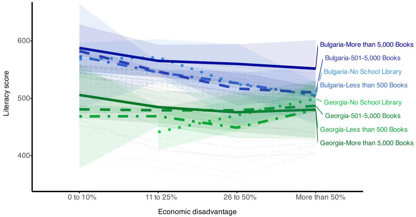
تقديرات التأثيرات العشوائية للمدرسة حسب البلد معقدة (الشكل 7): سنركز على تباين معين بين بلغاريا وجورجيا (النتائج الملونة في الشكل 7). هذه المقارنة مثيرة للاهتمام لأن هذين البلدين يبدو أنهما لديهما أنماط مختلفة من تفاعل المكتبة والحرمان الاقتصادي (الشكل 4). النمط الأكثر وضوحًا الذي يظهر في مخطط التفاعل (الشكل 4) هو أن الطلاب من بلغاريا (الخطوط الزرقاء) لديهم
4. المناقشة
. النماذج منخفضة الرتبة قادرة على ملاءمة التأثيرات العشوائية ذات الأبعاد الكبيرة جدًا: على سبيل المثال، قام Niku وآخرون (2019) بملاءمة GLVM بأبعاد 985 لمجموعة بيانات ميكروبية. عند ملاءمة النماذج لمجموعات بيانات أكبر، يمكن مواجهة صعوبات؛ على سبيل المثال، في علم البيئة، يكون عدد الأنواع غالبًا كبيرًا مقارنة بعدد العينات. في مثل هذه الحالات، قد يكون من المفيد ملاءمة نموذج عدة مرات مع قيم بدء مختلفة للمعلمات، ويعتبر الملاءمة ذات أعلى قيمة للاحتمالية اللوغاريتمية هي أفضل نموذج ملاءمة.
خطوة رئيسية في تطبيق تأثير عشوائي منخفض الرتبة هي اختيار الرتبة
هيكل الرتبة المنخفضة له نقطة اختلاف مثيرة للاهتمام عن الطرق الأخرى لملاءمة تأثير عشوائي متعدد المتغيرات حيث يسمح بمصفوفة تباين-تغاير مفردة، أو بشكل أكثر دقة، يفترض التفرد. تتطلب الطرق الأخرى لملاءمة التأثيرات العشوائية المرتبطة مصفوفة تباين-تغاير إيجابية محددة وتعيد تحذيرات عند مواجهة (قرب) التفرد، وهي مشكلة تم تجاوزها هنا من خلال افتراض هيكل منخفض الرتبة.
تقدم أمثلتنا لمحات قليلة فقط عن كيفية استخدام هياكل التباين-التغاير منخفضة الرتبة في النمذجة المختلطة، حيث كان من الصعب تقنيًا ملاءمة نماذج بتأثيرات عشوائية ذات أبعاد عالية. بعض المجالات التي نرى فيها استخدامًا محتملاً لهذا النهج تشمل التحليل العاملي مع تصاميم متعددة المستويات أو قياسات متكررة، وتحليل تفاعل الجين مع البيئة (Piepho 1997؛ Smith وآخرون 2001). نرى العديد من التطبيقات المحتملة، ونتطلع إلى رؤية كيف سيتم استخدام هذه الأداة الجديدة في الممارسة العملية.
References
Van der Veen B, Hui FKC, Hovstad KA, Solbu EB, O’Hara RB (2021). “Model-Based Ordination for Species with Unequal Niche Widths.” Methods in Ecology and Evolution, 12(7), 1288-1300. doi:10.1111/2041-210x. 13595.
أ. ملخصات النموذج لمثال مزرعة الرياح
R> summary(glmer(abundance ~ Zone + Year + (Species + 0 | ID),
+ family = "poisson", data = wf.ex))
Generalized linear mixed model fit by maximum likelihood (Laplace
        Approximation) ['glmerMod']
    Family: poisson ( log )
Formula: abundance ~ Zone + Year + (Species + 0 | ID)
            Data: wf.ex
            AIC BIC logLik deviance df.resid
        1310.5 1336.1 -648.3 1296.5 277
Scaled residuals:
            Min 1Q Median 3Q Max
-1.38779 -0.67079 0.06129 0.43556 1.58605
Random effects:
    Groups Name Variance Std.Dev. Corr
    ID SpeciesTorsk 0.7603 0.8719
                SpeciesTanglake 0.9839 0.9919-0.74
Number of obs: 284, groups: ID, 142
Fixed effects:

begin{tabular}{lrrrrr}
& Estimate & Std. Error & z & value & $operatorname{Pr}(>|z|)$ \
(Intercept) & 0.63001 & 0.10942 & 5.758 & $8.52 mathrm{e}-09$ & $* * *$ \
ZoneN & 0.07242 & 0.12807 & 0.565 & 0.57174 & \
ZoneS & -0.57875 & 0.19527 & -2.964 & 0.00304 & $* *$ \
Year2010 & 0.57457 & 0.10360 & 5.546 & $2.92 mathrm{e}-08$ & $* * *$
end{tabular}
---
Signif. codes: 0 '***' 0.001 '**' 0.01 '*' 0.05 '.' 0.1 ' ' 1
Correlation of Fixed Effects:
                (Intr) ZoneN ZoneS
ZoneN -0.343
ZoneS -0.525-0.014
Year2010-0.493 0.057-0.130
R> summary(glmmTMB(abundance ~ Zone + Year + (Species + 0 | ID),
+ family = "poisson", data = wf.ex))
    Family: poisson ( log )
Formula: abundance ~ Zone + Year + (Species + 0 | ID)
Data: wf.ex
| AIC | BIC | logLik deviance | df.resid | |
| 1310.5 | 1336.1 | -648.3 | 1296.5 | 277 |
Random effects:
Conditional model:

begin{tabular}{lllll}
Groups & Name & Variance & Std.Dev. & Corr \
ID & SpeciesTorsk & 0.7603 & 0.8719 & \
& SpeciesTanglake & 0.9839 & 0.9919 & -0.74
end{tabular}
Number of obs: 284, groups: ID, 142
Conditional model:

begin{tabular}{lrrrrl}
& Estimate & Std. Error z value & $operatorname{Pr}(>|z|)$ & \
(Intercept) & 0.63000 & 0.10942 & 5.758 & $8.53 e-09$ & $* * *$ \
ZoneN & 0.07243 & 0.12807 & 0.566 & 0.57170 & \
ZoneS & -0.57876 & 0.19528 & -2.964 & 0.00304 & $* *$ \
Year2010 & 0.57457 & 0.10360 & 5.546 & $2.92 e-08$ & $* * *$
end{tabular}
---
Signif. codes: 0 '***' 0.001 '**' 0.01 '*' 0.05 '.' 0.1 ' ' 1
ب. تحليل البوتستراب البرامترية لمثال مزرعة الرياح
R> LRobs <- 2 * logLik(wf.glmm) - 2 * logLik(wf.glmm.null)
R> library("boot")
R> lrt.fun <- function(data) {
+ library("glmmTMB")
+ null <- try(glmmTMB(abundance ~ Zone + Year +
+ diag(Zone + Year|Species) +
+ (1|Station) + rr(Species + 0 | ID, d = 2),
+ family = "poisson", data = data))
+ alt <- try(glmmTMB(abundance ~ Zone * Year + diag(Zone * Year|Species) +
+ (1|Station) + rr(Species + 0 | ID, d = 2),
+ family = "poisson", data = data))
+ LR <- tryCatch({2 * logLik(alt) - 2 * logLik(null)},
+ error = function(e) {NA})
+ return(LR)
+ }
R> sim.abund <- function(data, mle) {
+ library("glmmTMB")
+ out <- data
+ out$abundance <- simulate(mle)$sim_1
+ out
+ }
R> wf.boot <- boot(data = windfarm, ran.gen = sim.abund, lrt.fun,
+ mle = wf.glmm.null, sim = "parametric", R = 1000, parallel = "snow",
+ ncpus = 4)
R> p <- (sum(wf.boot$t[,1] >= LRobs, na.rm = TRUE) + 1)/(1000 + 1)
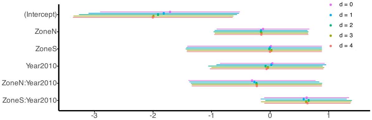
ج. تحليل الحساسية
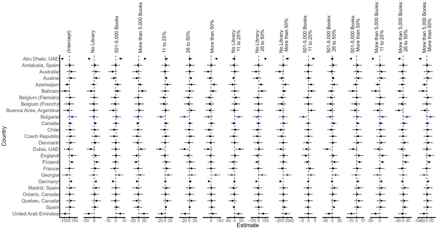
د. تقديرات التأثير العشوائي ذو الرتبة المخفضة من نموذج PIRLS
الانتماء:
جامعة UNSW سيدني
مدرسة الرياضيات والإحصاء ومركز أبحاث التطور والبيئة
NSW 2052، أستراليا
البريد الإلكتروني: m.mcgillycuddy@unsw.edu.au
جامعة UNSW سيدني
مركز الإحصائيات، مركز مارك وينرايت التحليلي
NSW 2052، أستراليا
جامعة مكماستر
قسم الرياضيات والإحصاء
1280 الشارع الرئيسي الغربي
هاميلتون، أونتاريو L8S 4K1، كندا
DOI: https://doi.org/10.18637/jss.v112.i01
Publication Date: 2025-01-01
Parsimoniously Fitting Large Multivariate Random Effects in glmmTMB
Abstract
Multivariate random effects with unstructured variance-covariance matrices of large dimensions,
1. Introduction
R> glmer(abundance ~ Zone + Year + (Species + 0 | ID), family = "poisson",
+ data = windfarm)
R> glmmTMB(abundance ~ Zone + Year + (Species + 0 | ID), family = "poisson",
+ data = windfarm)
One common way to deal with high dimensionality is to use a reduced-rank approach, making simplifying assumptions that reduce the dimension of the problem to
GLVMs have been used frequently in ecology and the social sciences, early examples being models of the presence-absence of fish species (Walker and Jackson 2011) and of polytomous party choice and rankings data (Skrondal and Rabe-Hesketh 2003). GLVMs can be technically challenging to fit, but there are a number of dedicated software solutions. The gllamm package (Rabe-Hesketh, Skrondal, and Pickles 2004) in Stata (StataCorp 2023) uses adaptive Gaussian quadrature to integrate out the latent variables. Early software written in R , with ecologists in mind, used Bayesian Markov chain Monte Carlo (Hui 2016; Ovaskainen et al. 2017). Substantially faster fits can be obtained using a Laplace (Huber, Ronchetti, and Victoria-Feser 2004; Niku, Warton, Hui, and Taskinen 2017) or variational approximation (Hui, Warton, Ormerod, Haapaniemi, and Taskinen 2017) to the marginal likelihood, as implemented in the R package gllvm (Niku et al. 2019). These tools were written with a particular model in mind, where a multivariate random intercept is used to induce correlation across many responses, and fixed effects are used to relate the linear predictor to measured variables, although there have been some extensions to relax this constraint in different ways (Van der Veen, Hui, Hovstad, Solbu, and O’Hara 2021; Niku, Hui, Taskinen, and Warton 2021). However, this software is unable to handle a range of common sampling designs. An example considered in Section 3.2 is when the multivariate random effect has covariates that may vary across and within clusters.
In this paper we add reduced-rank functionality to the glmmTMB package (Brooks et al. 2017) for flexible mixed effects models that can include factor analytic terms, for multivariate
random effects of large dimension. The glmmTMB package, available from the Comprehensive R Archive Network (CRAN) at https://CRAN.R-project.org/package=glmmTMB, is built as an extension to lme4 (Bates et al. 2014), widely used in the applied sciences for problems involving a range of study designs, including multi-level and repeated measures designs. The glmmTMB package uses a similar interface to lme4 but exploits automatic differentiation for faster estimation of mixed effects models (Brooks et al. 2017). By adding reduced-rank functionality to glmmTMB, we enrich the class of mixed models that can be fitted to include multivariate random effects with much larger dimension than was previously possible, such that we can now routinely fit random effects of dimension in the hundreds, or perhaps in the thousands. This new class of models includes, for example, GLVMs with functionality for any of the study designs that can be analysed using lme4, including multi-level or repeated measures designs.
Section 2 provides an overview of the generalized linear mixed model, the factor analytic extensions to handle multivariate random effects of high dimension, and the estimation approach used in glmmTMB to fit such models. We describe the usage of glmmTMB to fit reduced-rank multivariate random effects. We analyse two different data sets, from ecology and the social sciences, in Section 3. Section 4 concludes the paper.
2. Methods
2.1. Models
with the number of parameters in
A reduced-rank approach to fit a multivariate random effect involves expressing it as a linear function of
Given these definitions, the multivariate random effect is distributed as
2.2. Estimation
We focus on the Laplace approximation of the marginal likelihood, which is widely used for GLMMs (Raudenbush, Yang, and Yosef 2000) as well as GLVMs (Huber et al. 2004; Niku et al. 2017). By writing Equation 3 in the form
can be written as
In glmmTMB we maximize a Laplace approximation of the marginal log-likelihood obtained from the package Template Model Builder (TMB) (Kristensen, Nielsen, Berg, Skaug, and Bell 2015) in R (or more precisely, minimize the negative log-likelihood). TMB evaluates the Laplace approximation and its derivatives using automatic differentiation. Any gradientbased optimization method available in R can be used to do the maximization, by default glmmTMB uses nlminb(). TMB then uses the generalized delta method to calculate marginal standard deviations of fixed and random effects (Kass and Steffey 1989).
2.3. Software interface
rr(x | group, 2)
So for example to model the mean of a response ( y ) as a function of x and let the coefficients of x vary randomly among groups as a function of two latent variables, the formula is
The non-negative integer after the comma in the formula specifies the number of latent variables, or rank, of the variance-covariance matrix of the multivariate random effects, which defaults to
One issue with fitting a factor-analytic model is that the likelihood function is often multimodal, which may lead to convergence to a local maximum. To overcome this we include a data-driven method based on the work of Niku et al. (2019) to initialize values for parameters so that the maximizing algorithm starts closer to the global maximum. The default in glmmTMB sets parameter values to zero, or one for fixed-effect parameters for some link functions. To control the algorithm used for initializing parameters a start_method argument, specified as a list with components method and jitter.sd, has been added to
glmmTMBControl(). Setting method = “res” fits a generalized linear model (GLM) to the data to obtain estimates of the fixed parameters, which are then used as starting values of the fixed parameters. From the fitted model, residuals are calculated for models using the Poisson, negative binomial, and binomial families using the method due to Dunn and Smyth (1996), while the internal function dev.residuals is used for other families. Starting values for latent variables,
More examples of implementing the rr structure are shown in Section 3. Information on the reduced-rank and other available variance-covariance structures in glmmTMB can be found in vignette(“covstruct”, package = “glmmTMB”).
3. Application
3.1. Wind farm data
A multivariate random effect is required to account for correlation in species responses within a sample – we expect correlation across species due to inter-specific interactions, or response to unobserved environmental conditions (Warton et al. 2015) and we wish to be able to estimate positive or negative correlations. We do not have any a priori structure for this correlation, and for nine species we would require 45 parameters to estimate the variance-covariance matrix among species. Thus we would expect considerable instability in the fit, especially for correlation terms involving rarer species. In comparison, a reduced-rank covariance structure of rank two would require only 17 parameters.
We model abundances,
R> glmmTMB(abundance ~ Zone * Year + diag(Zone * Year | Species) +
+ (1 | Station) + rr(Species + 0 | ID, 2), family = "poisson",
+ control = glmmTMBControl(start_method = list(method = "res")),
+ data = windfarm)
glmmTMB.
| Conditional model: | ||||||||||
| Groups | Name | Std.Dev. | Corr | |||||||
| ID | SpeciesTanglake | 0.4741 | ||||||||
| SpeciesTorsk | 0.1618 | 0.40 | ||||||||
| SpeciesStensnultra | 0.6963 | 0.36 | 1.00 | |||||||
| SpeciesOxsimpa | 0.2092 | -1.00 | -0.34 | -0.29 | ||||||
| SpeciesAL | 0.5502 | -0.85 | 0.13 | 0.18 | 0.89 | |||||
| SpeciesRotsimpa | 0.8684 | 0.24 | 0.99 | 0.99 | -0.17 | 0.30 | ||||
| SpeciesSkrubbskadda | 0.6541 | 0.43 | 1.00 | 1.00 | -0.36 | 0.10 | 0.98 | |||
| SpeciesSandskadda | 1.6886 | 0.39 | 1.00 | 1.00 | -0.32 | 0.14 | 0.99 | 1.00 | ||
| SpeciesSjurygg | 0.6395 | 0.52 | 0.99 | 0.98 | -0.46 | 0.00 | 0.95 | 0.99 | 0.99 | |
3.2. PIRLS data
We propose that students from economically disadvantaged schools (Eco_disad) with a library containing more books (Size_lib) have higher literacy scores than students from a school with no library, but the difference in literacy scores will be less when students are from schools of higher economic background i.e., there is an interaction between the two school variables. Further, we would like to know how the interactive effect of these school-level variables will vary by country, hence we want to fit a random slopes model, with different Eco_disad:Size_lib effects for each country. Both Eco_disad and Size_lib are categorical variables with four levels, hence we need 15 parameters to characterize their joint effect and a 15-dimensional random effect in the model. Estimating an unstructured variance-covariance matrix
We consider the model for literacy score,
This model can be fitted in glmmTMB using the following command:
R> glmmTMB(Overall ~ Size_lib * Eco_disad + (1 | School) +
+ rr(Size_lib * Eco_disad | Country, d = 3),
+ control = glmmTMBControl(start_method = list(method = "res")),
+ family = gaussian(), data = pirls)
The conditional estimates of the school random effects by country are complex (Figure 7): we will focus on a particular contrast between Bulgaria and Georgia (colored results in Figure 7). This comparison is of interest because these two countries appear to have different patterns of library-economic disadvantage interaction (Figure 4). The most obvious pattern shown in the interaction plot (Figure 4) is that students from Bulgaria (blue lines) have
4. Discussion
model. Reduced-rank models are capable of fitting random effects of very large dimension: for example, Niku et al. (2019) fitted a GLVM with a dimension of 985 to a microbial data set. When fitting models to larger data sets, difficulties can be encountered; for example, in ecology the number of species is often large compared to the number of samples. In situations like this, it may be useful to fit a model multiple times with different starting values for the parameters, and the fit with the highest log-likelihood value is considered the best fitting model.
A key step in applying a reduced-rank random effect is choosing the rank
The reduced-rank structure has an interesting point of difference from other approaches to fitting a multivariate random effect in that it permits a singular variance-covariance matrix, or more precisely, it assumes singularity. Other methods of fitting correlated random effects require a positive-definite variance-covariance matrix and return warnings when encountering (near-)singularity, an issue circumvented here by assuming a reduced-rank structure.
Our examples give just a few tastes of how reduced rank variance-covariance structures can be used in mixed modelling, where it has previously been technically difficult to fit models with random effects of high dimension. Some example areas where we see potential use for this approach include factor analysis with multi-level designs or repeated measures, and genotype-by-environment interaction analysis (Piepho 1997; Smith et al. 2001). We see a myriad of potential applications, and look forward to seeing how this new tool is used in practice.
References
Van der Veen B, Hui FKC, Hovstad KA, Solbu EB, O’Hara RB (2021). “Model-Based Ordination for Species with Unequal Niche Widths.” Methods in Ecology and Evolution, 12(7), 1288-1300. doi:10.1111/2041-210x. 13595.
A. Model summaries for the wind farm example
R> summary(glmer(abundance ~ Zone + Year + (Species + 0 | ID),
+ family = "poisson", data = wf.ex))
Generalized linear mixed model fit by maximum likelihood (Laplace
        Approximation) ['glmerMod']
    Family: poisson ( log )
Formula: abundance ~ Zone + Year + (Species + 0 | ID)
            Data: wf.ex
            AIC BIC logLik deviance df.resid
        1310.5 1336.1 -648.3 1296.5 277
Scaled residuals:
            Min 1Q Median 3Q Max
-1.38779 -0.67079 0.06129 0.43556 1.58605
Random effects:
    Groups Name Variance Std.Dev. Corr
    ID SpeciesTorsk 0.7603 0.8719
                SpeciesTanglake 0.9839 0.9919-0.74
Number of obs: 284, groups: ID, 142
Fixed effects:

begin{tabular}{lrrrrr}
& Estimate & Std. Error & z & value & $operatorname{Pr}(>|z|)$ \
(Intercept) & 0.63001 & 0.10942 & 5.758 & $8.52 mathrm{e}-09$ & $* * *$ \
ZoneN & 0.07242 & 0.12807 & 0.565 & 0.57174 & \
ZoneS & -0.57875 & 0.19527 & -2.964 & 0.00304 & $* *$ \
Year2010 & 0.57457 & 0.10360 & 5.546 & $2.92 mathrm{e}-08$ & $* * *$
end{tabular}
---
Signif. codes: 0 '***' 0.001 '**' 0.01 '*' 0.05 '.' 0.1 ' ' 1
Correlation of Fixed Effects:
                (Intr) ZoneN ZoneS
ZoneN -0.343
ZoneS -0.525-0.014
Year2010-0.493 0.057-0.130
R> summary(glmmTMB(abundance ~ Zone + Year + (Species + 0 | ID),
+ family = "poisson", data = wf.ex))
    Family: poisson ( log )
Formula: abundance ~ Zone + Year + (Species + 0 | ID)
Data: wf.ex
| AIC | BIC | logLik deviance | df.resid | |
| 1310.5 | 1336.1 | -648.3 | 1296.5 | 277 |
Random effects:
Conditional model:

begin{tabular}{lllll}
Groups & Name & Variance & Std.Dev. & Corr \
ID & SpeciesTorsk & 0.7603 & 0.8719 & \
& SpeciesTanglake & 0.9839 & 0.9919 & -0.74
end{tabular}
Number of obs: 284, groups: ID, 142
Conditional model:

begin{tabular}{lrrrrl}
& Estimate & Std. Error z value & $operatorname{Pr}(>|z|)$ & \
(Intercept) & 0.63000 & 0.10942 & 5.758 & $8.53 e-09$ & $* * *$ \
ZoneN & 0.07243 & 0.12807 & 0.566 & 0.57170 & \
ZoneS & -0.57876 & 0.19528 & -2.964 & 0.00304 & $* *$ \
Year2010 & 0.57457 & 0.10360 & 5.546 & $2.92 e-08$ & $* * *$
end{tabular}
---
Signif. codes: 0 '***' 0.001 '**' 0.01 '*' 0.05 '.' 0.1 ' ' 1
B. Parametric bootstrap analysis for the wind farm example
R> LRobs <- 2 * logLik(wf.glmm) - 2 * logLik(wf.glmm.null)
R> library("boot")
R> lrt.fun <- function(data) {
+ library("glmmTMB")
+ null <- try(glmmTMB(abundance ~ Zone + Year +
+ diag(Zone + Year|Species) +
+ (1|Station) + rr(Species + 0 | ID, d = 2),
+ family = "poisson", data = data))
+ alt <- try(glmmTMB(abundance ~ Zone * Year + diag(Zone * Year|Species) +
+ (1|Station) + rr(Species + 0 | ID, d = 2),
+ family = "poisson", data = data))
+ LR <- tryCatch({2 * logLik(alt) - 2 * logLik(null)},
+ error = function(e) {NA})
+ return(LR)
+ }
R> sim.abund <- function(data, mle) {
+ library("glmmTMB")
+ out <- data
+ out$abundance <- simulate(mle)$sim_1
+ out
+ }
R> wf.boot <- boot(data = windfarm, ran.gen = sim.abund, lrt.fun,
+ mle = wf.glmm.null, sim = "parametric", R = 1000, parallel = "snow",
+ ncpus = 4)
R> p <- (sum(wf.boot$t[,1] >= LRobs, na.rm = TRUE) + 1)/(1000 + 1)
C. Sensitivity analysis
D. Reduced-rank random effect estimates from PIRLS model
Affiliation:
UNSW Sydney
School of Mathematics and Statistics and Evolution & Ecology Research Centre
NSW 2052, Australia
E-mail: m.mcgillycuddy@unsw.edu.au
UNSW Sydney
Stats Central, Mark Wainwright Analytical Centre
NSW 2052, Australia
McMaster University
Department of Mathematics & Statistics
1280 Main Street West
Hamilton, Ontario L8S 4K1, Canada