رؤية شبكة التنسور لطرق هارتري متعددة الطبقات ومتعددة التكوين المعتمدة على الزمن A tensor network view of multilayer multiconfiguration time-dependent Hartree methods

المجلة: Molecular Physics، المجلد: 122، العدد: 14
DOI: https://doi.org/10.1080/00268976.2024.2306881
تاريخ النشر: 2024-02-12

رؤية شبكة التنسور لطرق هارتري متعددة الطبقات ومتعددة التكوين المعتمدة على الزمن

هنريك ر. لارسونقسم الكيمياء والكيمياء الحيوية، جامعة كاليفورنيا، ميرسيد، كاليفورنيا 95343، الولايات المتحدة الأمريكية*

الملخص

طريقة هارتري متعددة الطبقات ومتعددة التكوينات المعتمدة على الزمن (ML-MCTDH) ومجموعة إعادة تنظيم مصفوفة الكثافة (DMRG) هما أداتان قويتان تُستخدمان بشكل رئيسي في مجالات علمية مختلفة. على الرغم من أن كلا الطريقتين تستندان إلى حالات الشبكة التنسورية، إلا أن لغات رياضية مختلفة تمامًا تُستخدم لوصفهما. هذا يحد بشدة من نقل المعرفة وأحيانًا يؤدي إلى إعادة اختراع أفكار معروفة جيدًا في المجال الآخر. هنا، نستعرض نظرية ML-MCTDH وDMRG باستخدام تعبيرات MCTDH ومخططات الشبكة التنسورية. نستنتج معادلات الحركة لـ ML-MCTDH باستخدام المخططات ونقارنها بخوارزميات DMRG المعتمدة على الزمن وغير المعتمدة على الزمن. كما نستعرض تقدمين حديثين مختارين. التقدم الأول يتعلق بتحسين دوال الجسيمات الفردية غير المشغولة في MCTDH، والتي تت correspond إلى إثراء الفضاء الفرعي في DMRG. التقدم الثاني يتعلق بالعثور على هياكل شجرية مثالية وتسليط الضوء على أوجه التشابه والاختلاف في الشبكات التنسورية المستخدمة في نظريات MCTDH وDMRG. نأمل أن يسهم هذا المساهمة في تعزيز تبادل الأفكار بشكل أكثر إنتاجية بين ML-MCTDH وDMRG.

المقدمة

تم تطوير طريقة هارتري متعددة التكوينات المعتمدة على الزمن (MCTDH) ومجموعة إعادة تنظيم مصفوفة الكثافة (DMRG) تقريبًا في نفس الوقت في مجالات الديناميات الكمية الجزيئية وفيزياء المادة المكثفة، على التوالي. . لقد أثرت الطريقتان بشكل كبير على مجالهما المعني ولا تزالان تفعلان ذلك. يمكن رؤية ذلك بوضوح من خلال ملاحظة أن MCTDH و DMRG يتم استخدامهما خارج مجالهما البحثي الأول وأصبحا الآن راسخين في مجالات أخرى مثل الهيكل الإلكتروني الجزيئي من البداية [5-8] في حالة DMRG وديناميات الإلكترون في الحقول القوية في حالة MCTDH [9-15]، من بين العديد من الأمثلة الأخرى. في البداية، كانت MCTDH وDMRG تركزان على مجالات وتطبيقات مختلفة تمامًا. تعتمد MCTDH على معادلة شرودنجر الزمنية (TDSE) بينما تعتمد DMRG على معادلة شرودنجر المستقلة عن الزمن (TISE). بعد حوالي 20 عامًا من تأسيسهما، تم توسيع كلا الطريقتين. تم تحسين دالة الموجة الأقل مرونة لـ MCTDH (بالنسبة لـ DMRG)، وهي تحليل تاكر [16]، من خلال تطوير طريقة MCTDH متعددة الطبقات (ML-MCTDH) [17-19]، حيث يتم استخدام حالة شبكة موتر شجرية (TTNS) أو تنسيق تاكر الهرمي [20-26]. بالنسبة لـ DMRG، تم توسيع التركيز على TISE من خلال التمديدات إلى التطور في الزمن الحقيقي [27-30]. علاوة على ذلك، تم لاحقًا توسيع دالة الموجة لـ DMRG، وهي حالة منتج المصفوفات (MPS) [31-35]، والتي هي مجموعة فرعية من TTNSs، إلى TTNSs [36-40]. استلهمت طرق أخرى من DMRG التي توسع TTNSs لتشمل حالات الشبكة التنسورية العامة (TNSs) [41-50]. أدت هذه التطورات الفردية المختلفة إلى لغات رياضية مختلفة تمامًا تُستخدم لوصف DMRG وML-MCTDH وMPSs وTTNSs. في الواقع، وصف DMRG باستخدام MPSs هو مفهوم أكثر حداثة يختلف بشكل كبير عن لغة DMRG الأصلية [35، 51]. هذه الحواجز اللغوية تزداد حدة مع استخدام المزيد والمزيد من أساليب DMRG في أنظمة تُعالج عادةً باستخدام (ML-)MCTDH والعكس صحيح [52-72]. من الصعب جدًا تحليل أوجه التشابه والاختلاف بين الأساليب التي طورتها هاتان الجماعتان، حتى عندما تكون هذه الأساليب مشابهة جدًا أو متطابقة تقريبًا.
هنا، مع التركيز على ML-MCTDH، سنسلط الضوء على الروابط بين ML-MCTDH و DMRG من خلال “ترجمة” تعبيرات MCTDH إلى اللغة التخطيطية التي تُستخدم على نطاق واسع في مجتمع TNS ولكن لم يتم استخدامها بالكامل حتى الآن في مجتمع ML-MCTDH. نأمل أن تُظهر هذه الترجمات الروابط بشكل أوضح بين ML-MCTDH و DMRG و TNSs. سنبرز قوة اللغة التخطيطية من خلال اشتقاق معادلات الحركة لـ ML-MCTDH عبر الرسوم البيانية. سنناقش طريقة بديلة لحل معادلات الحركة لـ ML-MCTDH، والتي تُعطى من خلال أساليب DMRG المعتمدة على الزمن وغير المعتمدة على الزمن. علاوة على ذلك، سنظهر الروابط بين تقدمات DMRG و ML-MCTDH التي يتم توضيحها من خلال موضوعين متقدمين، (1) إثراء الفضاء الفرعي (وظائف الجسيمات الفردية غير المشغولة المثلى، SPFs)، و (2) هياكل TTNS المثلى، والتي تتضمن أيضًا مناقشة حول سبب تفضيل MPSs في بنية الإلكترونيات الجزيئية، مقارنةً بـ TTNSs في الديناميات الكمومية الاهتزازية.
مخططنا كالتالي: الأقسام II و III تستعرض بإيجاز لغات ML-MCTDH وشبكات التنسور، على التوالي. الأقسام IV و V “تترجم” التعبيرات القياسية (ML-)MCTDH ومعادلات الحركة ML-MCTDH، على التوالي. القسم VI يستخرج بالكامل معادلات الحركة ML-MCTDH باستخدام الرسوم البيانية فقط. القسم VII يستعرض إجراءات التوحيد/التعامد TTNS وعمليات المسح النموذجية لـ DMRG. يتم استعراض نهج DMRG المعتمد على الزمن والذي يمكن اعتباره نظيرًا لمعادلات ML-MCTDH في القسم VIII ويستخدم لوصف DMRG المستقل عن الزمن.
في القسم التاسع. يتناول القسمان العاشر والحادي عشر موضوعين متقدمين حول SPFs غير المشغولة وتحسينات هيكل الشجرة. نختتم في القسم الثاني عشر.

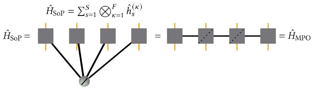
II. الاقتراح متعدد الطبقات ومتعدد التكوينات المعتمد على الزمن هارتري

لحل معادلة شرودنجر، فإن الطريقة القياسية للتفاعل الكامل (FCI) هي فرضية ريتز-غاليركين [26،77]، حيث أن دالة الموجة ذات الأبعاد – تمثل بواسطة حاصل ضرب مباشر لـ “أسس بدائية” ذو حجم محدود في كل بُعد :
هنا، نستخدم تدوين ديراك [78، 79] ونفترض وجود قاعدة أولية متعامدة. علاوة على ذلك، سنناقش فقط حالة الجسيمات القابلة للتمييز (أو تحويل مناسب للجسيمات غير القابلة للتمييز، مثل تحويل جوردان-ويجنر) وبالتالي لا نفترض أي تناظر (أو عدم تناظر) في موتر المعاملات ذو القيم الحقيقية أو المعقدة. التي سيتم تحديد مدخلاتها بعد ذلك.
في معظم تطبيقات الديناميات الكمية الجزيئية، تكون القاعدة الأولية هي قاعدة شبكية طيفية أو شبه طيفية تُعطى بواسطة تمثيل المتغيرات المنفصلة (DVR) [80-85]، والتي تُعرف، من بين أمور أخرى، أيضًا بطريقة شبكة لاغرانج [86] في بعض الأدبيات الفيزيائية وكقاعدة كاردينال في بعض الأدبيات الرياضية التطبيقية [84، 87]. لاحظ أن القواعد غير الخطية، وخاصة القواعد الغاوسية، ممكنة أيضًا [88، 89].
الافتراض FCI في المعادلة (1) دقيق في فضاء الأساس البدائي (بافتراض عدم وجود تقريبات إضافية على هاميلتونيان) ولكن عدد المدخلات في موتر المعامل يتناسب كـ ، حيث هو المتوسط الهندسي لأحجام الأساس لتجنب هذا التوسع المفرط، يقوم نموذج (ML-)MCTDH بتقريب المعادلة (1) عن طريق التوسع في قاعدة متعامدة أخرى، تُسمى دوال الجسيم الفردي (SPFs) الفرق بين الأساس البدائي وأساس SPF هو أن الأخير يتم تحسينه بطريقة تباينية وبالتالي يتطلب عددًا أقل من دوال الأساس. ثم يأخذ اقتراح (ML-)MCTDH الشكل التالي
لاحظ أن SPFs قد تكون متعددة الأبعاد (لذا ); انظر أدناه. الرقم العلوي 1 في وفي تشير إلى الطبقة في ML-MCTDH. بالنسبة لتطور الزمن، كلا من موتر بُعدي وتم تحسين دوال الحالة الذاتية وفقًا لمبدأ التباين الزمني المعتمد على ديراك-فرينكل-ماكلخلان (TDVP) [90-94].
بعض الملاحظات حول الرموز المستخدمة هنا: من أجل التناسق مع النص الرئيسي للأدبيات المتعلقة بـ ML-MCTDH، نتبع هنا عن كثب ولكن ليس حصريًا الرموز المستخدمة من قبل مانثي [19، 95]. إنها تختلف بشكل طفيف فقط عن تلك المستخدمة من قبل ماير وفيندرل [96]، ولكن هناك بعض الاختلافات عن الرموز المستخدمة من قبل وانغ وثوس (على سبيل المثال، يختلف عد الطبقات) [18، 97]. ومن الجدير بالذكر أن جميع هذه الرموز تستند إلى الصيغ الأصلية لـ MCTDH [1،2]. توجد رموز مختلفة في مجتمع الرياضيات [98-102]. يتم تقديم مقارنة غير شاملة للرموز المستخدمة في مجتمعات MCTDH والرياضيات وشبكات التنسور في الجدول I.
الافتراض في المعادلة (2) مرن جداً وهناك ثلاث realizations رئيسية له: (1) في أبسط افتراض MCTDH، تكون الدوال الأساسية الذاتية أحادية البعد و ثم يتم تمثيل SPFs بنفس الأساس البدائي المستقل عن الزمن المستخدم في فرضية FCI، المعادلة (1). وبالتالي، فإن MCTDH له نفس التوسع الأسي مثل فرضية FCI، ولكن القاعدة تقل حيث يتم تحسين SPFs وبالتالي يحتاج عدد أقل منها، مقارنة بالأساس البدائي.
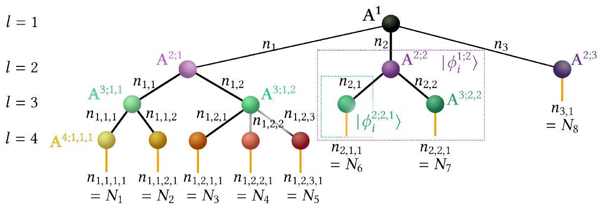
(2) بالنسبة لـ MCTDH مع مجموعة الأوضاع [103]، ويتم التعبير عن SPFs من حيث متعدد الأبعاد ( أساس) متعدد الأبعاد. عادةً ما يكون هذا الأساس أساسًا من نوع المنتج المباشر، ولكنه يمكن أن يكون أيضًا أساسًا غير منتج مباشر [104-106]. يتم الإشارة إلى درجات الحرية متعددة الأبعاد التي تصف SPFs متعددة الأبعاد على أنها “منطقية”. يعتبر دمج الأوضاع مفيدًا لوصف درجات الحرية المرتبطة بقوة. بالنسبة للأنظمة التي تحتوي على غالبًا ما يؤدي دمج الأوضاع إلى كفاءة أفضل من طريقة MCTDH العادية. في سياق بنية الجزيئات الإلكترونية، فإن طريقة MCTDH المضادة للتناظر مع دمج الأوضاع تعادل خوارزمية المجال الذاتي المتسق النشط الكامل المعتمد على الزمن (TD-CASSCF) [107-111]. يُطلق على هذا أيضًا اسم هارتري-فوك متعدد التكوين المعتمد على الزمن، MCTDHF [9-15]. في TD-CASSCF،
الجدول I. بعض الرموز المستخدمة في هذا العمل وفي أدبيات MCTDH. يتم تقديم قائمة غير شاملة من الرموز البديلة المستخدمة في أدبيات MCTDH والرياضيات وDMRG أيضًا. انظر الشكل 1 للحصول على مثال ملموس على استخدام بعض الرموز.
وصف رمز رموز بديلة
البعد الفيزيائي
حالة الأساس الفيزيائية (“البدائية”)
البعد الأساسي الفيزيائي
عدد الطبقات ل
طبقة
حالة أساس SPF
الموضع الأفقي في الطبقة
موضع العقدة/SPF
موضع الطبقة والعقدة/SPF
موضع موتر المعامل
بعدد العقد/الموتر/الموقع/أبعاد SPF
حجم السند/الرتبة/أساس SPF
حجم قاعدة SPF العامة
الحجم الإجمالي للأساس الذي يمثل SPF
مؤشر SPF
مؤشر SPF المركب
مؤشر SHF المركب
موتر SPF/موقع
تكوين
وظيفة الثقب الواحد (SHF)
تكوين SHF
جهاز عرض SPF
جهاز عرض SHF
مصفوفة كثافة الجسيم الفردي
مشغل الحقل المتوسط
مشغل القياس
حد هاملتوني أحادي البعد
ستسمى الدوال الثلاثية الأبعاد التي تصف إلكترونًا واحدًا بالأوربيتال الجزيئي، وستسمى الدوال الأساسية البدائية بالأوربيتال الذري.
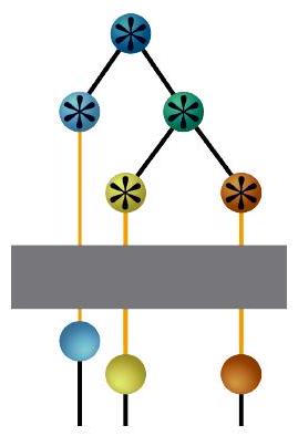
(3) بالنسبة لـ ML-MCTDH، يظل كذلك، لكن يتم توسيع SPFs ذات الأبعاد في المعادلة (2) بشكل متكرر باستخدام نفس فرضية MCTDH، أي أن
ثم يتم وصفها إما بواسطة الأساس البدائي (ربما مع دمج الوضع) أو يتم توسيعها مرة أخرى باستخدام فرضية MCTDH. يتم تكرار ذلك بشكل متكرر حتى الطبقة الأخيرة. تم الوصول إلى.
يمكن تمثيل الهيكل التكراري لأسلوب ML-MCTDH باستخدام مخططات شجرية كما هو موضح في الشكل 1، الذي يقدم أيضًا مثالًا على بعض رموز ML-MCTDH. في سياق ML-MCTDH، تُستخدم هذه المخططات تقريبًا بشكل حصري لتصوير الهيكل الشجري لوظيفة موجية معينة من ML-MCTDH. فقط مؤخرًا تم استخدامها لتمثيل بعض الكميات الأخرى المتعلقة بـ MCTDH. كما سنظهر أدناه في القسم الثالث، هناك ارتباط مباشر بين هذه المخططات الخاصة بـ ML-MCTDH ومخططات الشبكة التنسيلية المستخدمة في أدبيات DMRG. من بين أمور أخرى، سنظهر كيف يمكن استخدام هذه المخططات لاشتقاق معادلات الحركة لـ ML-MCTDH.
في التدوين المستخدم بشكل شائع، SPFs بُعدية من الطبقة يتم الإشارة إليها بـ . الرموز الإضافية، حدد الموقع الدقيق لنقاط SPF في الشجرة. المؤشرات تُحدد من خلال استكشاف الشجرة باستخدام البحث المتعمق بدءًا من . خلال التنقل، كانت الوضعية الأفقية للمسار عبر الشجرة المتخذ في الطبقة يتم إعطاؤه بواسطة .
لتجنب التعامل مع التدوين المزدحم المستخدم في فهرسة وتحديد مواقع التنسورات والدوال في
الشكل 1. مثال على شجرة ML-MCTDH/TTNS تعرض التدوين. الروابط (الرؤوس) التي تشير إلى المؤشرات الفيزيائية المقابلة لدوال الأساس الأولية تظهر باللون البرتقالي. حجمها موضح بـ ولكن أيضًا بشكل ضمني من خلال تظهر السندات التي تشير إلى مؤشرات “افتراضية” لوظائف الجسيم الفردي (SPFs) باللون الأسود. الشجرة لديها طبقات. أحجامها الأساسية هي أبعادهم هي ، وإجمالي عدد SPFs في عقدة واحدة هو . لاحظ أن SPF يتم وصفه بواسطة الموتر وأولئك من العقد السفلية المتصلة بـ بعض من دوال الشكل المحدد (SPFs) ومؤشرات معامل دوال الشكل المحدد (SPF coefficient tensors) موضحة أيضًا. يتم تمييز المؤشرات التي تصف دوال الشكل المحدد (SPFs) معينة بمستطيلات منقطة.
شجرة، غالبًا ما يبسط مطورو MCTDH الرموز من خلال تعريف الفهرس المركب ، الذي يحدد مدخلات الموترات اعتمادًا على السياق، يمكن أيضًا تحديد فهرس مفكك مع نطاق مع
نقوم بتبسيط الرموز أكثر من خلال تعريف المؤشرات المركبة ، و يحدد الطبقة والموقع ل SPF، و ذلك الخاص بمؤشر SPF. تؤدي هذه الصياغة المبسطة إلى وصف أكثر اختصارًا للـ SPFs على أنها
أين
هي التكوينات.
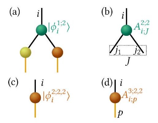
مسلحين بهذه التدوين المبسط، نقدم نظير SPFs، وظائف الثقب الواحد والتي يتم تعريفها من خلال إسقاط SPFs المقابلة إلى حالة ML-MCTDH أي،
باستخدام شروط التوافقية للأشكال الأساسية المتعامدة، يمكننا وصف كنتيجة لمجموع حاصل ضرب SHFs و SPFs،
تعتبر SHFs مفيدة لتعريف المشغلين الفعالين، كما هو موضح أدناه في القسم V A.
في لغة DMRG التقليدية [4، 35، 51]، المعادلة (8) تت correspond إلى استخدام DMRG لموقع واحد وتوسيع الحالة من حيث كتلة النظام، وكتلة البيئة، :
حيث يتم تمثيل كتلة النظام في تدوين MCTDH بواسطة SHFs وكتلة البيئة يتم تمثيلها بواسطة SPFs.
الشكل 2. مثال على رسم خريطة لموتر إلى عقدة تحتوي على أربعة رؤوس/روابط في مخطط شبكة التنسور. توضح الألواح (ب)-(د) رموزًا إضافية تم تقديمها هنا لتحديد المرافق المعقد (ب)، ومشتق الزمن (ج)، والتنسورات القطرية (د).
الشكل 3. مثالان على انقباضات التنسور. تظهر التنسورات الفردية، ومخططات الشبكة التنسورية الفعلية، حيث يتم ربط الروابط/الرؤوس التي تتوافق مع المؤشرات التي يتم الانقباض عليها، بالإضافة إلى المعادلات الرياضية. (أ) يظهر انقباض حالة MCTDH/تحليل تنسور تاكر. (ب) يظهر مدخل ناتج المصفوفتين ، و .

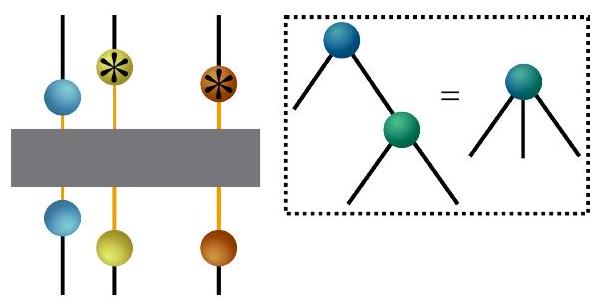
III. مخططات الشبكة التنسورية

نمط الانكماش التنسوري الكامل لاسترجاع حالة ML-MCTDH الكاملة/TTNS الممثلة بواسطة الأساس البدائي من التنسورات/تمثيلات SPF يتم تقديم ذلك فعليًا من خلال الرسم البياني الموضح في الشكل 1. هذا ممكن من خلال إدخال وسيلة لترجمة هذه الأنواع من مخططات الشبكات التنسورية إلى معادلات رياضية. منذ القرن التاسع عشر، وصف العلماء جبر التنسور باستخدام الرموز الرسومية [117-119]؛ انظر المرجع [120] للحصول على نظرة عامة. تم استخدام مخططات الشبكات التنسورية لأول مرة من قبل بينروز في الخمسينيات [121] ويمكن أن تكون مفيدة للغاية ليس فقط لتصورها ولكن أيضًا لاشتقاق التعبيرات الرياضية [30، 35، 47، 48، 122، 123]. تؤدي فكرة الشبكات التنسورية إلى TNSs. في مخطط الشبكة التنسورية، يتم تمثيل كل تنسور كعقدة ويتم تمثيل كل من مؤشرات التنسور كحواف أو “روابط؛” انظر الشكل 2 للحصول على مثال تمثيلي. غالبًا ما يتم تقديم بعض التعريفات الإضافية. في ما يلي، تشير النجمة فوق العقدة إلى المرافق المعقد. النقطة تشير إلى المشتق الزمني لتنسور وخط قطري يشير إلى التنسورات القطرية، كما هو موضح في الشكل 2. نظرًا لأن TTNS هو فرضية دالة الموجة لطريقة ML-MCTDH، سيتم استخدام مصطلحي TTNS و ML-MCTDH state بالتبادل في ما يلي.
مماثل لاتفاقية جمع آينشتاين [124]، يتم تعريف انقباضات التنسورات (الجمع على المؤشرات المشتركة) من خلال ربط الروابط المشتركة (الحواف) لتلك العقد التي يجب أن يتم انقباض مؤشراتهم المقابلة. الشكل 3 يوضح مثالين.
رسوم الشبكات التنسورية ليست مفيدة فقط لتصور انقباضات التنسور، بل يمكن استخدامها أيضًا لاشتقاق المعادلات وللدلالة على خصائص معينة. الشكل 4 يظهر مثالاً على حساب مشتقة شبكة تنسورية من خلال رسم.

الرابع. مخططات الشبكة التنسورية مقارنة بلغة MCTDH

بهدف مقارنة لغة MCTDH مع مخططات التنسور، نقدم هنا ترجمة للتعبيرات الشائعة الاستخدام في MCTDH. سنستخدم حالة ML-MCTDH / TTNS الموضحة في الشكل 5 كمثال. لاحظ أنه، نظرًا لمرونة TTNSs من حيث هيكلها، فإن معادلات TTNS يتم تمثيلها بشكل أفضل بمساعدة أشجار الأمثلة. التعميمات إلى هياكل شجرية أخرى بسيطة. هذا يختلف عن MPSs أو حالات الأزواج المتشابكة المتوقعة، حيث أن تلك TNSs لها هياكل أبسط (شبكات أحادية أو ثنائية الأبعاد، على التوالي).
الشكل 4. مثال على كيفية استخدام المخططات لاشتقاق التعبيرات الرياضية. يظهر هنا مشتق شبكة التنسور من الشكل 3 (أ) بالنسبة إلى ، أي، .
الشكل 5. مثال على شجرة ML/TTNS المستخدمة هنا لاشتقاق تعبيرات ML-MCTDH. تحتوي TTNS على ثلاث طبقات وتصف حالة ثلاثية الأبعاد.
في مخطط TTNS، تُسمى المؤشرات التي تمثل الروابط الحرة “المعلقة”، أي التي لا تتصل بعقدة أخرى، بالفيزيائية. في مخططات الشبكة التنسورية، تُسمى جميع الروابط الأخرى في TTNS بالافتراضية. لا يمكن دائمًا تمييز الروابط الفيزيائية والافتراضية مباشرة في التعبيرات التخطيطية الأكثر عمومية ويجب استنتاجها من TTNS الأولي. لتبسيط ذلك، في المخططات التالية، سنقوم دائمًا بتلوين الروابط الفيزيائية باللون البرتقالي والروابط الافتراضية باللون الأسود. هنا، لكل موتر لونه المحدد، كما هو موضح في الشكل 5. في مخططات الشبكة التنسورية، عدد SPFs، يتوافق مع بعد السند ومن ثم يُطلق عليه أيضًا بعد السند (أحيانًا أيضًا مرتبة في الرياضيات أو عدد الحالات المحتفظ بها، ، بلغة DMRG التقليدية؛ قارن مع الجدول الأول). في ما يلي سنستخدم عند الإشارة إلى بُعد الرابطة/عدد الدوال الموجية الأساسية بشكل عام و عند الإشارة إلى عقدة معينة. يتم إعطاء أبعاد الروابط الفيزيائية كما هي في الأساس البدائي.
على عكس TTNS الكامل، فإن الوظائف مثل SPFs أو SHFs تحتوي على روابط افتراضية حرة. يجب أن تحتوي أي وظيفة على رابط مادي واحد أو أكثر، وعادةً ما تحتوي على رابط افتراضي حر واحد فقط يدل على رقم الوظيفة (على سبيل المثال، في ). تشير الروابط الفيزيائية بعد ذلك إلى قيم الدالة. غالبًا ما يتم تصوير الأورثونورمالية إما باستخدام الأسهم بدلاً من الروابط أو باستخدام رموز خاصة للعقد مثل المثلثات. هنا، نتبع الاتفاقية من ML-MCTDH وبعض الأدبيات الرياضية [23،26،98] ونصور الأورثونورمالية من خلال اتجاه الروابط الافتراضية. إذا كانت الرابطة الافتراضية تشير إلى الأعلى (نحو الطبقة 1، بعيدًا عن الروابط الفيزيائية)، فإن الدالة/التي tensor تكون أورثونورمالية. لاحظ أنه يوجد دائمًا رابطة افتراضية واحدة فقط تشير إلى الأعلى. إذا كانت الرابطة الافتراضية تشير إلى الأسفل (نحو الروابط الفيزيائية/الطبقة الأخيرة)، فإن الدالة/التي tensor تكون غير أورثونورمالية.
مثال على تكوين (مجموعة من SPFs/العقد) موضح في الشكل 6 مع انكماش التكوينات باستخدام موتر معامل، مما يؤدي إلى SPF. أمثلة على SPFs مقارنةً بموتيرات معامل فردية موضحة في الشكل 7. موتر معامل هو مجرد عقدة واحدة وروابطها المتصلة. قيم يمكن الحصول عليه من صناديق الاستثمار الخاصة
الشكل 6. مثال على التكوين. يظهر فيه من الشكل 5 في المستطيل المتقطع. انكماش لـ مع ، يؤدي إلى SPF .
الشكل 7. مخططات لـ SPFs مقارنة بالتنسورات. أربعة أمثلة على SPFs والتينسورات مأخوذة من الشكل 5 موضحة. (أ) و (ج) هما SPFs حيث تحتويان على روابط فيزيائية. (ب) و (د) هما موترات حيث تحتوي الرسوم البيانية فقط على عقدة واحدة. العقدة في (ج) متطابقة مع تلك في (د) ويمكن تفسيرها إما كـ SPF أو موتر، اعتمادًا على السياق.
الشكل 8. مثال على التحويل إلى مصفوفة والمصفوفات المتعامدة كرسوم بيانية. (أ) تحويل التنسور إلى مصفوفة إلى ، حيث هو مؤشر مركب لـ و . (ب) التدوين البياني للمتعامدية و، بشكل مكافئ، . الخط المستقيم يدل على مصفوفة وحدة.
عن طريق إسقاط جميع SPFs المتصلة بـ على قارن مع المعادلتين (5) و(6). لاحظ أنه بالنسبة للطبقة الأخيرة في الشجرة، يمكن تفسير العقدة إما كموتر أو كـ SPF، انظر الشكل 7 (ج) و(د). يعتمد التفسير المستخدم على السياق. يسمى موتر الجذر والعقدة المقابلة تسمى عقدة الجذر.
غالبًا ما يكون من المفيد إعادة تشكيل (وتبديل) موتر إلى مصفوفة، وهو ما يُسمى التماتُر (أو التسطيح أو نشر المصفوفة) [23]. على سبيل المثال، موتر بحجم يمكن أن يتم إعادة ترتيبها وإعادة تشكيلها في مصفوفة باستخدام الخريطة أين هو مؤشر مركب . هذا مفيد لتحقيق علاقات التعامد الطبيعي، على سبيل المثال، أو بشكل أكثر وضوحًا، و، بشكل مكافئ، الشكل 8 يقدم مثالاً على علاقات المصفوفة والعمودية في الرسوم البيانية.
في ML-MCTDH، تعني الأرتونورمالية لـ SPFs أن كل من التنسورات يمكن تحويل ما تم استخدامه لبناء SPFs في الرسم البياني إلى مصفوفات متعامدة. بحجم ، حيث هو الحجم الكلي لجميع الروابط الموجهة لأسفل، كما هو محدد في المعادلة (4). في هذه الحالة، يتم تنفيذ الماتريز باستخدام المؤشر المركب (المقابلة للرابطة الموجهة نحو الأسفل، نحو الروابط الفيزيائية) في كمؤشر صف ومؤشر SPF (السند يشير لأعلى نحو العقدة الجذرية) كمؤشر عمود؛ وبالتالي . هذا يؤدي إلى تبسيطات مفيدة للغاية للرسوم البيانية. على سبيل المثال، المعيار المربع لحالة ML-MCTDH، ببساطة يُعطى بواسطة موتر معامل عقدة الجذر، يوضح ذلك بشكل بياني في الشكل 9.
حساب التداخل، ، والمشروطة على فضاء SPF،
موضحة في الشكل 10. بسبب التوافق المتعامد، يقلل إلى . لاحظ أنه على الرغم من أن الدوال الأساسية الذاتية (SPFs) تكون متعامدة بشكل رسمي، إلا أن الدقة المحدودة لمحلل معادلة تفاضلية ML-MCTDH تؤدي إلى أخطاء صغيرة في عدم التعامد للدوال الأساسية الذاتية. في تطبيقات MCTDH، يتم تجاهل هذا الخطأ في عمليات الانكماش التنسوري، ولكن يتم تعديل مشروع الدالة الأساسية الذاتية لأخذ
الشكل 9. مخطط لتداخل TTNS مع نفسه (المعيار المربع). يتم استخدام TTNS من الشكل 5 كمثال. العلاقات الأورثونورمالية لـ SPFs تبسط المخطط بشكل كبير. قارن مع الشكل 8 (ب).
الشكل 10. تداخل SPF (أ) والإسقاط (ب). من الشكل 5 يُستخدم كمثال. بالنسبة لتداخل الدوال الذاتية المتعامدة، قارن مع الشكل 8 (ب).
أخذ الاعتبار للعدم التوافق الزائف من خلال [125]
أين هو مصفوفة التداخل لـ .
مثال على SHF موضح في الشكل 11. على عكس SPF، بالنسبة لـ SHF، فإن مؤشر الوظيفة يتوافق مع رابطة افتراضية موجهة نحو الأسفل (وليس نحو الأعلى) وبالتالي فإن SHF غير متعامدة. ومع ذلك، يمكن جعلها متعامدة؛ انظر القسم V A. العلاقة بين تحليل SHF-SPF في ML-MCTDH وتحليل النظام-البيئة في DMRG التقليدي، المعادلة (9)، موضحة في الشكل 12 (في هذه الحالة نقوم باستثناء ونظهر MPS بدلاً من TTNS من الشكل 5).
يمكن تعميم تعريف SHF ليشمل SHFs ذات الفهرسة المزدوجة المعرفة كما في [19]
حيث قمنا بتسليط الضوء على مؤشري “الثقب” الاثنين و حسب الألوان. يتم عرض مثال في الشكل 13. SHFs ذات الفهرسة المزدوجة
الشكل 11. مثال على دالة الثقب الواحد (SHF)، بناؤها واستخدامها. (أ) بناء SHF من الشكل 5 من خلال إسقاط على علاقات الأورثونورمال تسهل SHF، قارن مع الشكل 8 (ب). (ب) مبسط مع نظيرها، SPF تم التعاقد على يشكلون إجمالي TTNS .
الشكل 12. مقارنة بين مخطط ML-MCTDH ولغة DMRG التقليدية. (أ) تحليل حالة ML-MCTDH / MPS من حيث دالة ثقب مفرد (SHF) ودالة جسيم مفرد (SPF)؛ قارن مع الشكل 11. (ب) إعداد DMRG لموقع مفرد مع كتلة نظام وكتلة بيئة. كتلة النظام (البيئة) تمتد عبر فضاء SHF (SPF)؛ قارن مع المعادلة (9).
يسمح بتعريف تكراري لـ SHFs:
في الرسم البياني، يتم تمثيل SHF ذو الفهرسة المزدوجة ببساطة بواسطة رابطين افتراضيين، أحدهما يشير لأسفل والآخر يشير لأعلى؛ انظر الشكل 13 (ب).

V. معادلات ML-MCTDH والاتصال بالرسوم البيانية

تستند معادلات ML-MCTDH إلى فرضية ML-MCTDH، المعادلة (2)، وTDVP.
الشكل 13. مثال على دالة ثقب مفرد ذات فهرسة مزدوجة (SHF) واستخدامها. (أ) من الشكل 5 كمثال على SHF مزدوج الفهرسة. (ب) (انظر الشكل 11) مع تم التعاقد على ، يشكلون SHF .
الشكل 14. مخطط لمصفوفة كثافة الجسيم الفردي لنموذج TTNS من الشكل 5. قارن مع المعادلة (17).
أين يدل على التغيرات من الدرجة الأولى لـ فيما يتعلق بمعاييره. في ما يلي، سنقوم بتحديد بالنسبة لاقتراح دالة الموجة ML-MCTDH، يتم حل المعادلة (14) مع مراعاة قيودين: أولاً، شروط التوافق المتعامد للـ SPFs، وثانياً، عدم اعتمادها على القياس.
أين هو بعض مشغل قيود هيرميتي عشوائي و يدل على المشتقة الزمنية لـ تم مناقشة عدم التماثل في القياس بشكل أكبر في القسم السابع. باختصار، التحولات الوحدوية لـ SPFs/SHFs لا تغير لا التوافق المتعامد ولا الحالة. وهذا يؤدي إلى عدم تحديد SPFs الذي يتجلى من خلال عدم التماثل في القياس. يتم تثبيت هذا الغموض بواسطة المعادلة (15). خيارات متنوعة من يوجد وهنا، من أجل البساطة، سنستخدم واحدة من الخيارات الأكثر شيوعًا وسنجعلها ببساطة تساوي صفرًا [1]، أي،
تعميم المعادلات التالية إلى غير الصفر هو مباشر وسيتم مناقشة بعض جوانب استخدام مقياس مختلف في القسم الثامن.

أ. مصفوفات الكثافة والحقول المتوسطة
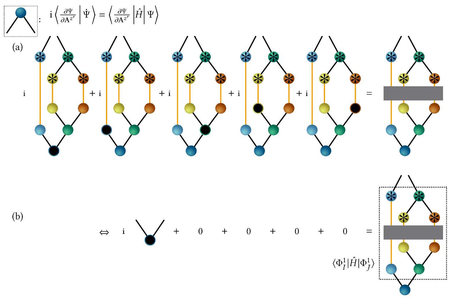
قبل أن نبدأ في تعريف معادلات الحركة، سنقوم بتعريف كميتين إضافيتين وتقديم تعبيرات بيانية لهما. يتم تعريف مصفوفة كثافة “الجسيم الفردي” على أنها
وهو يساوي المصفوفة المنقولة لمصفوفة الكثافة المخفضة لجسيم واحد في نظرية البنية الإلكترونية [111]. بالإضافة إلى ذلك، فإنه مرتبط بمصفوفة غرام. مع الإدخالات من مع المعلمات ، والذي يُستخدم في نظريات مشابهة [23،54،55،57،127،128]. تُبسط خاصية التعامد لـ SPF حساب ومثال على ذلك موضح في الشكل 14. إن تحويله إلى الشكل القطري ينتج عنه دوال شكل طبيعية ودوال شكل عشوائية. القيم الذاتية لـ تُسمى المهن الطبيعية. إن الـ SHFs ذات المهن الطبيعية غير الصفرية تكون متعامدة، ولكنها ليست متعامدة طبيعية.
تُعرّف مشغلات الحقل المتوسط على أنها
حيث قمنا بإدراج التعريفات لـ SHFs في المعادلة الثانية لتسليط الضوء على أن المعادلة (18) لا تزال تعرف مشغلاً وليس عددًا عدديًا. ومن ثم، هي مصفوفة من المشغلين. مثال على رسم بياني يبرز “جزء المشغل” و”جزء المصفوفة” (المؤشرات و ) من المعادلة (18) موضحة في الشكل 15.

ب. معادلات الحركة

باستخدام تعريفات مصفوفات الحقل المتوسط ومصفوفات الكثافة، نقدم الآن تعبيرات مختصرة لمعادلات الحركة في ML-MCTDH. تؤدي المعادلة (14) مع المعادلة (16) إلى المعادلات التالية للحركة للـ SPFs [2]:
الشكل 15. مخطط لمصفوفة الحقل المتوسط لنموذج TTNS من الشكل 5. المستطيل المتقطع يتوافق مع “جزء المشغل” من مصفوفة الحقل المتوسط وتحدد المؤشرات “جزء المصفوفة.” قارن مع المعادلة (18).
لاحظ أنه في الممارسة العملية، مصفوفة كثافة الجسيم الفردي يمكن أن تكون مفردة وعادة ما تحتاج إلى تنظيم [2]، ولكن توجد بدائل. ; انظر أيضًا القسم X. سنجعل المعادلة (19) أكثر وضوحًا من خلال إسقاط التكوينات المقابلة على المعادلة (19) بحيث يتم الحصول على معادلات الحركة لموتر معامل SPF كالتالي
لجذر الموتر في الطبقة الأولى نحصل على معادلات حركة شبيهة بمعادلات ريتز-غاليركين القياسية [26،77] لمعادلة شرويدنجر الزمنية المعتمدة، معبراً عنها في قاعدة محدودة (لكنها تعتمد على الزمن):

ج. بعض الأشكال الشائعة للهاميلتوني

أكثر شكل شائع من والمشغلين الآخرين المستخدمين من قبل MCTDH والعديد من الطرق الأخرى هو شكل مجموع المنتجات (SoP)، حيث يتم تحليل الهاميلتوني كمجموع لـ المنتجات المباشرة لمشغلات ذات بعد واحد:
في الجزء الثاني من المعادلة (22) قمنا بامتصاص المعاملات ذات القيم المركبة إلى أحد المشغلين ، من أجل الوضوح. هذه الهاميلتونية لها ميزة أن تطبيقها على حالة ما له تنفيذ بسيط نسبيًا ولكنه يتناسب بشكل جيد [131، 132] استنادًا إلى حلقة واحدة فقط على ضربات المصفوفات المحسّنة جيدًا [133].
النظير لمشغل هاملتونيان في مجتمع DMRG هو مشغل المنتج المصفوفي (MPO) [26،35،134،135]، والذي يُعرف بأنه
الـ MPO هو تعميم للـ MPS إلى مشغل. وبالمثل، يمكن تعريف مشغل شبكة موتر الشجرة كتعميق لـ TTNS إلى مشغل. في مجتمع MCTDH، يُعرف هذا بالنسبة لمشغلات الجهد القطرية بصيغة multilayer potfit، التي لم يتم استكشاف مزاياها وعيوبها بالكامل حتى الآن.
يمكن تمثيل هاملتونيان SoP كـ MPO يكون قطريًا في بعد الربط [138، 139]: تعريف كمؤشر مركب مفكك يمكن تحويل المعادلة (22) إلى المعادلة (23) من خلال العلاقة
يتم عرض هاملتونيان SoP ورسمه إلى MPO بشكل بياني في الشكل 16.
الشكل 16. مخطط لمشغل مجموع المنتجات (SoP) ورسمه إلى مشغل مصفوفة المنتج المحدد (MPO) مع موترات قطرية. هنا، تشير الخطوط المنقطة والقطرية في موترات MPO إلى موترات قطرية فقط بالنسبة لبُعد الربط الافتراضي (الخطوط السوداء). تشير الخطوط البرتقالية إلى الفضاء الفيزيائي. قارن مع المعادلات (22)-(24).
الشكل 17. مخطط لتمثيل مصفوفة لمشغل مجموع المنتجات في حقل متوسط لنموذج TTNS من الشكل 5. يتم تصور تقسيم هذا المخطط إلى مصطلح دالة ثقب واحد (جزء المصفوفة في الحقل المتوسط) ومصطلح تكوين (جزء المشغل في الحقل المتوسط) بواسطة مستطيلات منقطة. قارن مع المعادلة (26) والشكل 15.
بالنسبة لمعادلات ML-MCTDH، المعادلة (20)، من المفيد إعادة كتابتها من حيث المشغل الذي يعمل فقط على نفس الفضاء الذي تمتد إليه التكوينات ، ومن حيث المشغل الذي يعمل على المساحة المتبقية [19، 96]:
يتم تعريفه بشكل تكراري بنفس الطريقة التي يتم بها تعريف SPFs، مما يجعل هذا التقسيم مشابهًا لتوسع SHF-SPF لـ TTNS، المعادلة (8). يوجد تقسيم مطابق تقريبًا لـ DMRG وهذا التقسيم يتحقق بشكل تافه لكل من SoPs وMPOs. ثم يمكن تمثيل “المصفوفة” لمشغل الحقل المتوسط، المعادلة (18)، التي يتم إعطاؤها بواسطة موتر رباعي الأبعاد، على النحو التالي
يوضح الشكل 17 مثالاً على الرسم البياني. لاحظ أن كل من مشغلات الحقل المتوسط ومصفوفات الكثافة يمكن تقييمها بكفاءة بطريقة تكرارية بدءًا من الطبقة الأولى لجزء الكثافة وبدءًا من الطبقة الأخيرة لجزء المشغل [19]. هذا مرتبط بتقليص التداخلات من موقع إلى آخر في DMRG [35، 48].

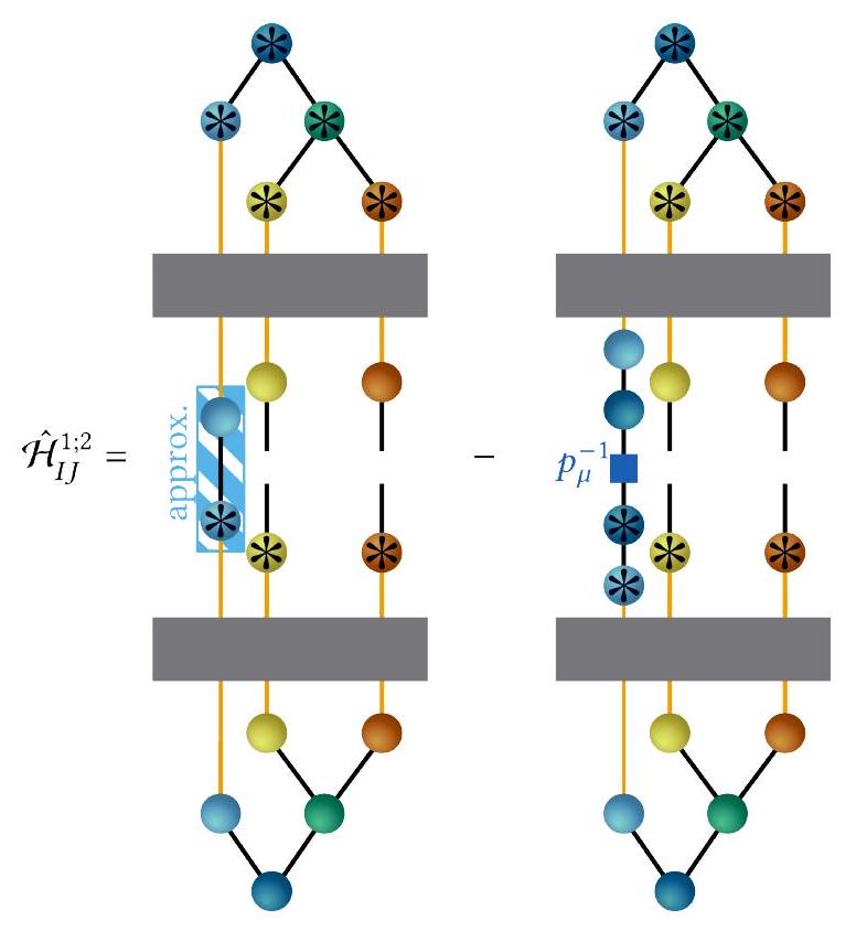
VI. اشتقاق ML-MCTDH باستخدام الرسوم البيانية

هنا سنستخدم مخططات الشبكة التنسورية لاستنتاج معادلات الحركة ML-MCTDH (20) و (21). لحل TDVP، نحتاج إلى التغيرات من الدرجة الأولى. إنها مرتبطة بمشتقات TTNS بالنسبة لجميع مكونات التنسورات الفردية، التي نحددها هنا على أنها :
الشكل 18. مشتقات TTNS. التغير من الدرجة الأولى لـ ، التي تحتوي على مشتقات بالنسبة إلى الموترات الفردية (اللوحة العلوية)، ومشتق الزمن (اللوحة السفلية) لـ TTNS من الشكل 5. يتم تمييز التنسورات التي تشير إلى التغيرات بعلامة .
إدراج إلى TDVP، المعادلة (14)، يؤدي إلى عدد من الحدود يساوي عدد المعلمات في TTNS لـ ، ونحصل على
نظرًا للاختلافات هي عشوائية ومستقلة عن بعضها البعض، يجب أن تتلاشى كل من الحدود في المعادلة (28) بشكل مستقل عن بعضها البعض ومستقل عن التغيرات [91]. ومن ثم، نحصل على مجموعة المعادلات التالية
هنا، سيكون من المفيد استخدام بنية التنسور لإعادة كتابة المعادلة (30) من حيث التنسورات الفردية لشبكة التنسور المتسلسلة.
مع شروط القياس المعادلة (16)، ستؤدي كل من هذه المعادلات إلى معادلات الحركة لتنسور معين.
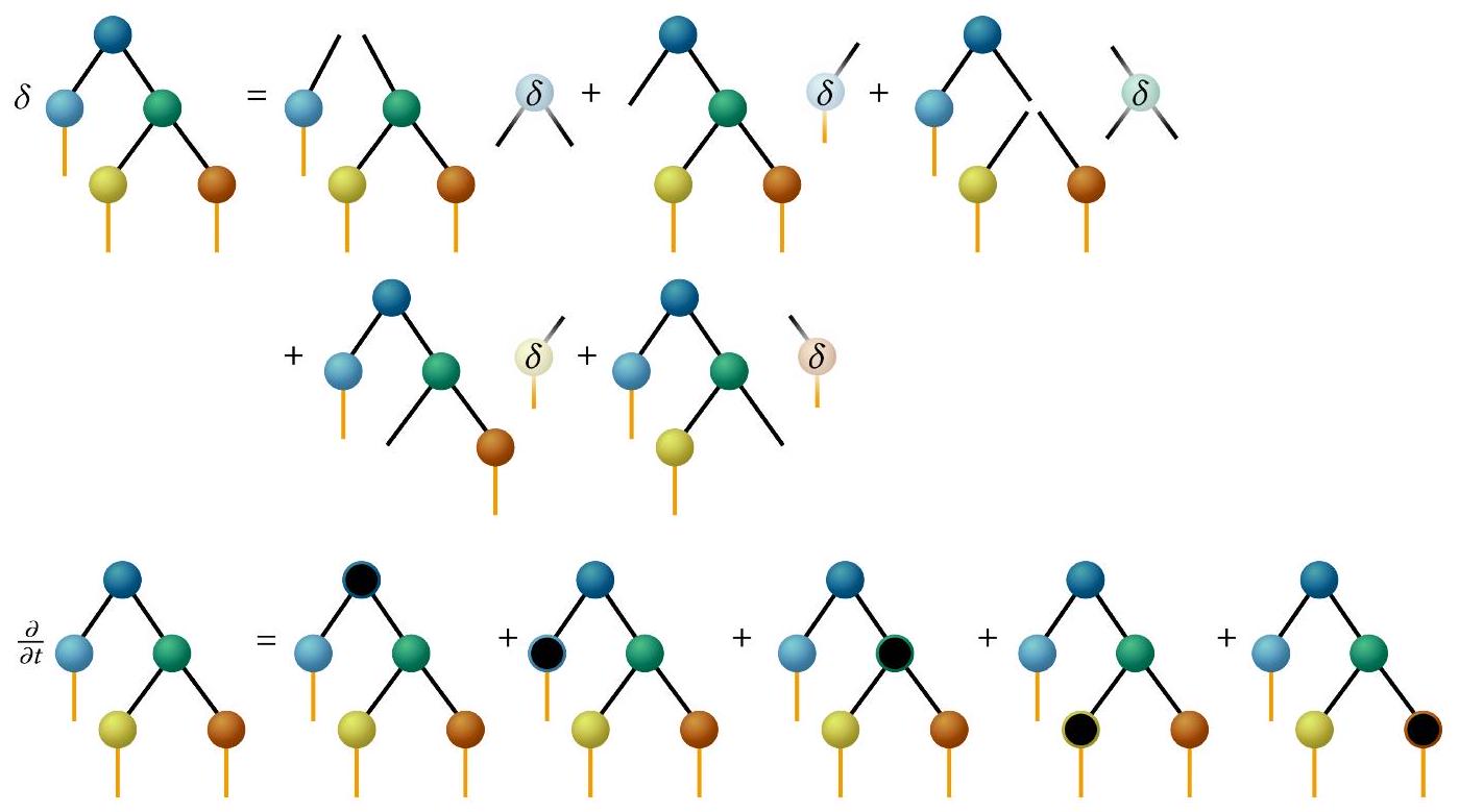
لاشتقاقات معادلات الحركة لكل موتر، نستخدم مرة أخرى TTNS من الشكل 5 كمثال بسيط ولكن نلاحظ أن هذا يمكن تعميمه بسهولة على أي TTNS، بما في ذلك TTNSs ذات طبقات أكثر. التغير من الدرجة الأولى والمشتقة الزمنية لـ موضحة في الشكل 18.
نبدأ الاشتقاق بالحد الأول من في الشكل 18، الذي يخص العقدة الجذرية، إدخال هذا في المعادلة (31) يؤدي إلى التعبير في الشكل 19(أ). لأننا نطلب أن يكون إسقاط SPF على مشتقته الزمنية صفرًا، المعادلة (16)، فإن معظم الحدود الناتجة عن تختفي، ومن خلال استخدام علاقات التعامد لـ SPF، الشكل 10، نحصل ببساطة على المعادلة (21)، التي تم توضيحها بيانيًا في الشكل 19(b).
بعد ذلك ننتقل إلى المعادلات لـ من TTNS في الشكل 5. يتم عرض الاشتقاق في الشكل 20. من خلال إدخال المعادلة (21) التي تم اشتقاقها للتو، نحصل على شكل محدد من المعادلة (20) لهذه العقدة. بالمقارنة مع المعادلة الأكثر عمومية (20)، هناك نوعان من التغييرات: أولاً، نظرًا لأن طبقة التالية لا يوجد لـ ، هنا التكوينات من المعادلة (21) تتوافق فقط مع تمثيل الأساس البدائي. ثانياً، في الشكل 20 قمنا بنقل إلى الجانب الأيسر في المعادلة (20)، والتي تقترب من اشتقاق MCTDH الأصلي وتلمح إلى طرق أخرى لحل هذه المعادلة، وهي باستخدام المعكوس الزائف لـ [1,130] (انظر
الشكل 19. اشتقاقات معادلات الحركة لمتجه الجذر (الموضح في المستطيل العلوي الأيسر) لـ TTNS من الشكل 5. يتم الإشارة إلى هاميلتونيان بواسطة المستطيل الرمادي. تأتي الحدود الفردية من الشكل 18. بعد الاستفادة من علاقات التعامد لـ SPF، الشكل 10، وقياس SPF، المعادلة (16)، يصل المرء إلى اللوحة (ب)، التي تتوافق مع المعادلة (21). يبرز المستطيل المنقط في الزاوية السفلى اليمنى من اللوحة (ب) .
أيضًا المراجع [127، 140] والقسم XA). لاحظ أن المعادلات التي تم اشتقاقها للتو لـ و كافية لبرمجة معادلات الحركة العادية لـ MCTDH بالكامل دون الشكل متعدد الطبقات.
المشتقات للمعادلات لـ يشبه إلى حد كبير كما هو موضح في الشكل 21. الفرق الرئيسي هو أنه هنا لدينا في الواقع تكوينات الظهور في المخططات. وذلك لأن ليس مرتبطًا بأي أساس بدائي، وهو ما يحدث فقط في ML-MCTDH وليس في MCTDH العادي للتنسورات غير الجذرية.
ننتقل الآن إلى الاشتقاقات الخاصة بالموترات في الطبقة الثالثة. بما أن ليس مختلفًا عن سنركز على واحد فقط منهم. إدراج إلى المعادلة (31) يؤدي إلى الرسوم البيانية الموضحة في الشكل 22. بالمقارنة مع الاشتقاق للطبقة الأولى والثانية، هنا يكون الاشتقاق أكثر تعقيدًا قليلاً حيث يتعين علينا أخذ معادلات الطبقتين السابقتين في الاعتبار. أولاً، نبسط مصطلحين يظهران على الجانب الأيسر من الشكل 22(b). لذلك، نجمع النتائج من الشكل 19 والشكل 21، مما يعطي التعبير الموضح في الشكل 23. لاحظ أن مصطلحين على الجانب الأيمن من الشكل 23 يلغي كل منهما الآخر. إدخال هذا مرة أخرى في الشكل 22(b) يؤدي إلى المعادلات النهائية للحركة كما هو موضح في الشكل 24. وهذا يتوافق مع المعادلة (20) للطبقة 3.
نلاحظ أنه بجانب النهج “القياسي” الذي نستخدمه هنا [ يوجد نهج بديل لاشتقاق معادلات الحركة لـ ML-MCTDH . هناك، يتم اشتقاق المشروع أولاً الذي يُسقط على الفضاء المماس، أي الفضاء الذي يمتد بواسطة التغيرات من الدرجة الأولى. ثم يتم حل
يمكن كتابته كـ ، حيث هو معكوس مصفوفة غرام. مع هذا التشكيل لـ يتم الحصول على معادلات الحركة القياسية ML-MCTDH [142-144]. باستخدام تعبير مختلف عن ستصبح هذه الطريقة مهمة لنظام TDVP-DMRG الم discussed في القسم الثامن.

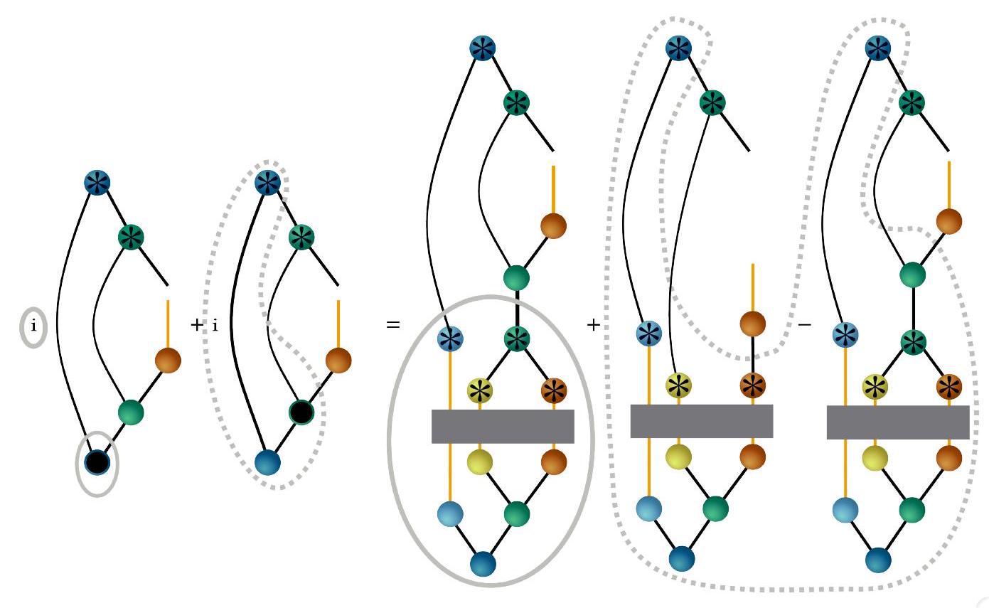
VII. التوحيد: تغيير العقدة الجذرية والتنظيف

هنا، سنناقش كيفية تغيير العقدة الجذرية لحالة ML-MCTDH/TTNS دون تغيير الحالة الفعلية الممثلة، والتي هي جوهر خوارزميات DMRG. هذه “التوحيد القياسي” تستغل أن TTNS غير متغيرة تحت
الشكل 20. اشتقاقات معادلات الحركة لـ (الموضح في المستطيل العلوي الأيسر) من TTNS الموضح في الشكل 5. تم تعيين الحدود التي تساوي صفر بشكل تافه بسبب شروط القياس إلى صفر على الفور (قارن مع الشكل 19). تم استخدام علاقات التعامد SPF، الشكل 10، والتعبير من الشكل 19 في اللوحة (ب) لتبسيط التعبير في (أ). وهذا ما تم تمييزه بالبيضاوات الرمادية.
الشكل 21. نفس الشكل 20 ولكن لـ .
الشكل 22. الجزء الأول من اشتقاق معادلات الحركة لـ (الموضح في المستطيل العلوي الأيسر) من TTNS الموضح في الشكل 5. تم تعيين الحدود التي تساوي صفر بشكل تافه بسبب شروط القياس إلى صفر على الفور (قارن مع الشكل 19). تبسط خاصية التعامد في SPF التعبير في (أ)، كما هو موضح في (ب) (قارن مع الشكل 9).
تحويل بواسطة مصفوفة قابلة للعكس . يتم رؤية ذلك من خلال إدخال في توسيع SHF، المعادلة (8):
حيث قدمنا -تحويل SHFs و SPFات ،
هذا موضح بشكل بياني في الشكل 25(أ).
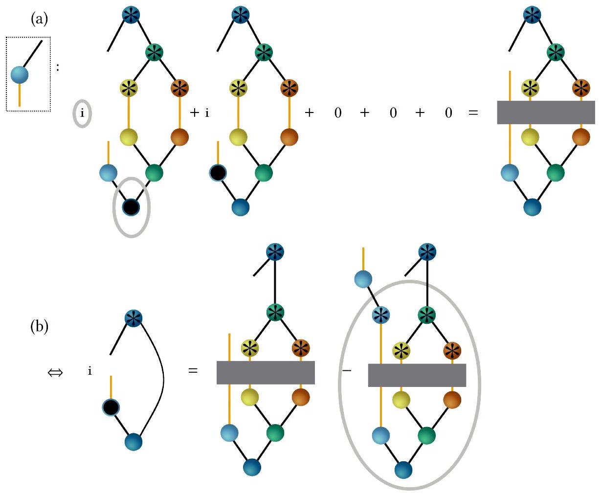
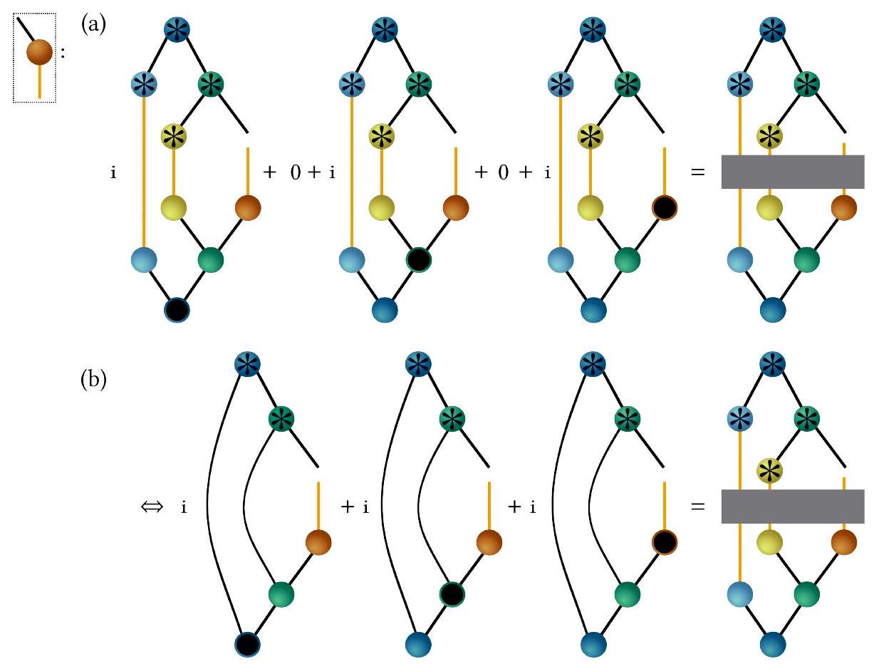
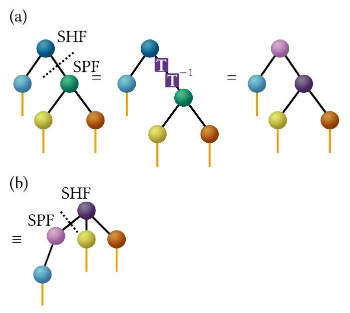
يمكن اختيار T لتعامد وتطبيع SHFs. وهذا يؤدي بعد ذلك إلى SPFs غير المتعامدة التي تم تحويلها بواسطة T. ومع ذلك، نظرًا لأن SPFs يجب أن تكون متعامدة وطبيعية، يمكننا الآن إعادة تفسير المعادلة (34) ببساطة من خلال تبادل معاني SHFs وSPFs المحولة بواسطة T عن طريق تحويل SHFs المتعامدة الآن إلى SPFs والعكس بالعكس. وهذا يؤدي إلى تغيير في هيكل الشجرة. بالإضافة إلى ذلك، إذا تم إجراء التحويل للطبقة الأولى، فإن عقدة الجذر تتغير. وهذا موضح في الشكل 25(b).
في الممارسة العملية، بسبب التوافق المتعامد لجميع دوال الشكل الأساسية في نظام الشبكة التنسيلية، لتوحيد وتطبيع دوال الشكل المتجانسة. يحتاج المرء فقط إلى جعل الموتر متعامدًا مع الإدخالات . يتم ذلك أولاً عن طريق نقله إلى مع الإدخالات ، حيث و تتوافق مع التسميات لهيكل الشجرة مع تغيير عقدة الجذر. ثم تم تحويله إلى مصفوفة (قارن مع الشكل 8) وتمت عملية التعامد. يمكن إجراء عملية تعامد المصفوفة وتطبيعها، على سبيل المثال، باستخدام تحليل المصفوفة QR، الذي يتوافق مع عملية تعامد غرام-شميدت [23، 145]. في مصفوفة QR ثم يتوافق مع في المعادلة (36) ويتم امتصاصه في الموتر المتصل بـ تُظهر هذه العملية، التي تُسمى أحيانًا التماثل [39]، مع الشروط المختلفة للأورثونورمال (التماثلات) لمتجه الجذر الأولي بشكل بياني في الشكل 26.
لاحظ أن هذا التغيير في التوحيد يمكن أن يتم مع أي زوج من SPF-SHF في الشجرة وليس فقط مع ذلك الخاص بالطبقة 1. علاوة على ذلك، يسمح لنا التوحيد بالتنقل بشكل منهجي في الشجرة بطريقة تجعل كل موتر في مرحلة ما يصبح على الأقل
الشكل 23. التعبير عن رسمين على الجانب الأيسر من الشكل 22(b). توضح البيضاويات ذات الخطوط الرمادية (المتقطعة الرمادية) التعبير من الشكل 19 (الشكل 21). لاحظ أن الحد الأول والأخير على الجانب الأيمن يلغي كل منهما الآخر.
الشكل 24. التعبير النهائي لمعادلات الحركة لـ (الموضح في المستطيل العلوي الأيسر) من TTNS الموضح في الشكل 5. للوصول إلى ذلك، يتم إدخال التعبير من الشكل 23 في الشكل 22.
مرة واحدة جذر العقدة. هذه مكونة مهمة في أي خوارزمية DMRG وتسمى المسح. يمكن تنفيذها باستخدام خوارزميات الرسم البياني مثل البحث المتعمق؛ انظر الشكل 27 لمثال. هناك طرق أخرى للتنقل في TTNS في مسح واحد ممكنة أيضًا [39].
ك remark تقني، بدلاً من استخدام تحليل QR لجعل SHFs متعامدة، يمكن أيضًا استخدام إجراءات أخرى للتعامد مثل تحليل القيم المفردة (SVD) [23،145] (باستخدام في تحليل القيمة المفردة كمصفوفة عمودية وSV كـ ). هذا يعادل استخدام القيم الذاتية لمصفوفة الكثافة المخفضة. ومن ثم، يؤدي ذلك إلى SPFs طبيعية، والتي غالبًا ما تؤدي إلى تحسين الأرقام، حيث أن الهاميلتونيان الممثل بواسطة قاعدة التكوينات غالبًا ما يكون مهيمنًا قطريًا. SPFs التي تقوم بتقطيع الجزء القابل للفصل من الهاميلتونيان هي خيار آخر شائع الاستخدام لتحسين الأرقام [146]. جميع هذه الخيارات تحقق قياسًا معينًا.

ثامناً. تقريب DMRG المعتمد على الزمن

تتمثل إحدى المشكلات الرئيسية في معادلات الحركة لـ ML-MCTDH في أنها يمكن أن تصبح غير خطية بشكل كبير. لذلك، يجب استخدام مدمجات متطورة من أجل انتشار فعال [94]. للتغلب على ذلك بالنسبة لـ MCTDH القياسي، استنادًا إلى رؤى تفيد بأن الدوال الأساسية الذاتية (SPFs) تتطور عادةً بشكل أبطأ من الدالة الموجية الفعلية، تم تطوير مدمج فعال يستهدف هيكل معادلات MCTDH وأطلق عليه اسم مدمج الحقل المتوسط الثابت (CMF) [125، 147]. حيث تتواجد معادلات الحركة لـ
الشكل 25. عدم الاعتماد على القياس في حالة ML-MCTDH/TTNS. (أ) إدخال مصفوفة وعكسه على رابط افتراضي لا يغير الحالة. مصفوفة التحويل وعكسه يُشار إليهما كمستطيلات بنفسجية. يتم امتصاصها في الأنسجة بنفسجية؛ قارن مع المعادلات (34)-(36). (ب) إذا يتم اختياره لتعامد وتطبيع الدوال الشكلية العليا ثم يتغير هيكل الشجرة وتتحول SHFs إلى SPFs والعكس صحيح؛ انظر النص للتفاصيل. الخطوط المنقطة تحدد انقسام SHFs وSPFs.
الشكل 26. تغيير عقدة الجذر (التوحيد) من الموتر إلى . (أ) الخطوات التي تم تنفيذها في التوحيد: (I) إعادة تشكيل وتحليل QR و (II) امتصاص في . هذا يؤدي إلى هيكل شجري مختلف. (ب) شروط التعامد (التحويلات) لـ للهيكلين الشجريين (الأشكال القياسية) حيث هي عقدة الجذر (يسار) وحيث هي عقدة الجذر (يمين). الخط المستقيم يدل على مصفوفة وحدة.
الشكل 27. مثال على مسح عبر شجرة. هنا، يتم تعريف المسح ليبدأ عند عقدة في الطبقة الأخيرة (أسفل اليسار). في كل “توقف” من المسح، الذي يتم الإشارة إليه بالأرقام، يتم تعامد الموتر المقابل، مما يغير الشكل القياسي للشجرة. هذا يعرف مسحًا للأمام. عكس الاتجاه يؤدي إلى مسح للخلف ينتهي عند العقدة التي تبدأ المسح للأمام.
تم فصل SPFs، المعادلة (19)، وتلك الخاصة بالموتر الجذري، المعادلة (21)، من خلال افتراض أن التكوينات، ومصفوفات الكثافة، والحقول المتوسطة ثابتة في الزمن أثناء الانتشار. هذه لها ميزة أن الموتر الجذري يمكن أن ينتشر باستخدام مروجات أسية قياسية [84] مثل مروج لانكزوس التكراري القصير (SIL) [148]. يؤدي انتشار SIL إلى تقديرات خطأ فعالة [125، 147]. ثم يتم حل المعادلات الخاصة بـ SPFs باستخدام مروج عام. يمكن أن تكون خطة تكامل CMF أسرع بمقدار ترتيب من نشر جميع موترات MCTDH في وقت واحد. الخطأ هو من ترتيب بالنسبة لخطوة الزمن التكيفية .
نظرًا لأن CMF مصمم لـ MCTDH العادي، فإن استخدامه المباشر لـ ML-MCTDH محدود بالطبقتين الأوليين في TTNS. بينما من حيث المبدأ يمكن توسيع فكرة CMF إلى أي طبقة في ML-MCTDH، إلا أنه ليس قويًا كما يمكن نشر الموتر الجذري فقط باستخدام مدمج أسّي. وبالتالي، قد لا يقدم المدمج القياسي CMF تحسينات كبيرة لـ TTNSs ذات الطبقات العديدة. مدمج نسميه هنا TDVP-DMRG يضع مدمج CMF في أقصى حد ويسمح باستخدام مدمجات أسية لجميع الموترات من خلال الاستفادة من المسحات [61، 100]. كانت فكرة TDVP-DMRG مدفوعة بالبحث عن طريقة بديلة لحل معادلات حركة MCTDH [99، 100]، لكنها تم تقديمها في عدة مجالات تقريبًا في نفس الوقت. وبالتالي، يُعرف أيضًا باسم مدمج تقسيم المشروع (PSI)-MCTDH [75، 101، 116، 143]، مدمج لوبيتش [76، 149] (المسمى على اسم مخترعه [99، 100، 102]) بالإضافة إلى “تدريب الموتر KSL” في حالة MPSs [141، 150]. تم استخدام TDVP-DMRG لأول مرة لـ MPSs (ولاحقًا لـ MCTDH القياسي [101، 102]). أول تطبيق لـ TDVP-DMRG على TTNSs الذي نعرفه هو المرجع [151]. للتحليل الرياضي، انظر المرجع [152]. لقد استخدمناه مؤخرًا للحالة الصعبة للديناميات ذات السعة الكبيرة لأيون زوندل المتقلب [70].
هنا، قبل رسم الاشتقاق، نشرح أولاً الأفكار الأساسية لـ TDVP-DMRG باستخدام حجج غير دقيقة بعض الشيء. نظرًا لأن TTNS يغير عقدة الجذر الخاصة به أثناء مسح TDVP-DMRG، فإن نظام تسمية ML-MCTDH، الذي يرتبط بعقدة جذر معينة، يصعب استخدامه. بدلاً من ذلك، سنستخدم رموزًا عامة مثل و للإشارة إلى الموترات. يتم عرض توضيح تخطيطي لشجرتنا النموذجية (الشكل 5) في الشكل 28. نبدأ المسح في الشكل 28(أ) بموتر في إحدى الطبقات الأخيرة، والذي نطلق عليه هنا . الخطوة الأولى في الانتشار في TDVP-DMRG، الشكل 28(ب)، تتبع خطة CMF وتنتشر إلى الزمن باستخدام المعادلة (21) مع تقريب التكوينات المستقلة عن الزمن .
بدلاً من اتباع خطة CMF وحل المعادلة المعقدة (20) لنشر الموتر المجاور لـ في الشكل 28(ج)، نقوم بتعامد باستخدام، على سبيل المثال، تحليل QR. هذا يعطي ، كما هو موضح في الشكل 28(د). ثم يتم استبدال بـ و ، وهي عقدة جديدة إضافية في الشجرة، انظر الشكل 28(هـ). لتغيير عقدة الجذر إلى ، نحتاج إلى امتصاص في . ومع ذلك، فإن في خطوة زمنية مختلفة عن . من أجل الحصول على أوقات متطابقة لـ و ، نفسر كعقدة جذر فعلية ونعيد نشر إلى ، كما هو موضح في الشكل 28(و) و (ز). يستخدم هذا النشر العكسي مرة أخرى معادلات MCTDH للموتر الجذري، المعادلة (21)، لكن لاحظ أن التكوينات المستخدمة في المعادلة (21) لنشر تصف أوقات نشر مختلفة، وهي للأجزاء من التكوينات المرتبطة بـ و للأجزاء من التكوينات المرتبطة بـ . بعد إعادة نشر يتم امتصاصه في ، الذي يصبح عقدة الجذر الجديدة لـ TTNS؛ انظر الشكل 28(ح). يتم تكرار الإجراء الموصوف: يتم نشر وتعامده، ويتم إعادة نشر الناتج من تحليل QR لـ وامتصاصه في عقدة الجذر الجديدة ؛ انظر الشكل 28(ط). يؤدي القيام بذلك لكل موتر في TTNS في النهاية إلى الحالة المعلنة بالكامل
نحن الآن نرسم اشتقاق TDVP-DMRG. لتبسيط التعبيرات، هنا نستخرجها فقط لـ MPSs، لكن تعميم خطة TDVP-DMRG للأشجار أمر مباشر، كما أظهرنا في الأشكال 26 و 28. يتوافق MPS مع شجرة خطية غير متوازنة، ولكل عقدة رابطين افتراضيين ورابط مادي واحد، باستثناء الموترات في النهاية، التي تحتوي فقط على رابط افتراضي واحد. يمكننا كتابة MPS بعدد أبعاد حيث يكون شكله القياسي (عقدة الجذر) مركزيًا عند البعد كـ
انظر الشكل 29(أ) لمثال تخطيطي. هنا نستخدم تدوين ML-MCTDH المعدل قليلاً حيث نضيف موقع عقدة الجذر/الشكل القياسي باستخدام وحيث أسقطنا التسمية للطبقة الأولى في الموتر الجذري و SPFs. لتغيير عقدة الجذر إلى البعد ، نقوم بتحليل QR للموتر الجذري كـ
ونستخدم كمعاملات توسيع لـ SPFs الجديدة لعقدة الجذر عند البعد (قارن مع الشكل 26):
الشكل 28. خطة TDVP-DMRG لـ TTNS من الشكل 5. تظهر الألواح (أ)-(ح) خطوات مختلفة في الخوارزمية لنشر الموتر الأول ولتغيير عقدة الجذر إلى الموتر المجاور . تظهر اللوحة (ط) TTNS للموترات المعلنة و . مع تغير هيكل الشجرة أثناء المسح، نستخدم هنا رموزًا عامة لتسمية موترات معينة. هنا، هو الموتر الوحيد الذي يحتوي على 3 روابط افتراضية. وبالتالي، أثناء المسح، سيظهر مرتين كعقدة جذر، لكنه سيتم نشره مرة واحدة فقط إلى الزمن ثم سيتم تخطيه في المرة التالية التي يكون فيها عقدة جذر أثناء المسح. هذه هي الاختلاف الرئيسي عند تطبيق TDVP-DMRG على TTNSs بدلاً من MPSs. انظر النص للتفاصيل.
الشكل 29. مثال على MPS وأجزاء من مشروع فضاء المماس لموتر MPS. (أ) مثال على التدوين المستخدم في المعادلة (37) لـ . (ب) المشاريع و لـ MPS الموضح في (أ). هذه المشاريع هي جزء من مشروع فضاء المماس، المعادلة (41). تستخدم المعادلة (40)، حيث تم استبدال بـ من المعادلة (39)، وبالتالي اللون المختلف لتلك العقدة.
باستخدام التي تم تشكيلها حديثًا، نحصل على حالة وسيطة مع كعقدة جذر:
التي تجمع بين و في TTNS واحد. يُعرف هذا التمثيل باسم الشكل القياسي للرابط في لغة MPS. إنه الشكل المستخدم لإعادة نشر في الشكل 28. يؤدي امتصاص في كما في الشكل 26 إلى تمثيل TTNS مع مركز/عقدة جذر التوحيد عند .
يستخدم TDVP-DMRG TDVP المكتوب من حيث مشروع فضاء المماس ، المعادلة (32)، باستخدام شكل خاص من الذي يستخدم أشكالًا قياسية مختلفة لـ MPS:
مع
انظر الشكل 29(ب) لمخططات أمثلة. لاحظ أن يستخدم SPFs من الشكل القياسي للرابطة، المعادلة (40). المجموع الأول في المعادلة (41) ينعكس على جميع TTNSs الممكنة التي تختلف فقط في موقع واحد (قارن مع التغيرات من الدرجة الأولى الموضحة في الشكل 18). المجموع الثاني يطرح جميع المكونات التي تتطابق مع الحالة الحالية [30]، باستثناء المقياس.
باستخدام المعادلة (41) وفرض وجود هاملتوني غير معتمد على الزمن، يمكننا بعد ذلك كتابة انتشار TDVP، المعادلة (32)، من الزمن إلى كـ [65، 141]
حيث قمنا بتقريب الأس باستخدام تقسيم لاي-تروتر. هذا يؤدي إلى المخطط الذي تم مناقشته أعلاه والمبين في الشكل 28 لـ TTNS. ينتشر للأمام عقد الجذر و ينتشر للخلف المصفوفات. لمزيد من التفاصيل حول اشتقاق جوانب مختلفة، نشير إلى . يمكن الحصول على تعبير مشابه للمعادلة (45) لـ TTNSs من خلال التأكد من أن التنسورات التي تحتوي على أكثر من رابطين افتراضيين في TTNS ستنتشر مرة واحدة فقط خلال عملية واحدة (يمكن تجاهل انتشار الزمن خلال لحظات العملية حيث تصبح هذه التنسورات عقد الجذر الجديدة) [116، 152، 153]؛ ومع ذلك، فإن إثبات رياضي لهذا مفقود [152]. باستخدام كخطوة زمنية ودمج المعادلة (45) مع عملية خلفية يؤدي إلى خطأ تقسيم لاي-تروتر من الدرجة . هذا من نفس الدرجة مثل ذلك الخاص بمجمع CMF. بالمقارنة مع مخطط CMF لـ MCTDH، لم يتم تنفيذ أي خطوة زمنية تكيفية حتى الآن وعادة ما يحتاج الأمر إلى تجربة خطوات زمنية مختلفة. باستخدام مخططات التركيب، يمكن تحقيق درجات أعلى أيضًا، لكن هذا لم يتم استكشافه حتى الآن.
حالة خاصة مثيرة للاهتمام من TDVP-DMRG التي تشبه أكثر ML-MCTDH من DMRG هي مخطط الانتشار “غير الهرمي” الذي قدمه ويكي ومانث [76]. هناك، استنادًا إلى SHFs المعاد توجيهها بواسطة لويدين [155] (باستخدام كمصفوفة تحويل)، يتم تعريف مشغل مقياس زمني ومتعتمد على العقدة الذي يؤدي إلى معادلات حركة متناظرة لـ SHFs وSPFs. هذا يجعل جميع SHFs متعامدة وSPFs غير متعامدة. تأخذ معادلات الحركة لجميع التنسورات شكلًا مشابهًا لذلك الخاص بالتنسور الجذري، المعادلة (21)، بالإضافة إلى مصطلح إضافي للمشغل :
معًا مع التوجيه لويدين، فإن هذه المصطلحات الإضافية لمشغل المقياس لكل بعد من تتوافق تقريبًا مع التحلل والانتشار الخلفي لـ التنسور في TDVP-DMRG، وهنا مقيد ليكون . وبالتالي، بالمقارنة مع TDVP-DMRG، لا يوجد تقسيم لاي-تروتر ولكن بدلاً من ذلك، بسبب المقياس المداري المحدد، يصبح الهاملتوني الفعال معتمدًا على الزمن. بينما يتم الاستفادة من أفكار DMRG (استغلال مخططات التعامد المختلفة)، فإن هذا الناشر سهل التنفيذ باستخدام أكواد MCTDH الموجودة. علاوة على ذلك، لديه خاصية جذابة تتمثل في أنه يمكن نشر جميع التنسورات في وقت واحد باستخدام مجمع CMF مع خطوة زمنية تكيفية. هذا يجعل تنفيذ الناشر متوازيًا بشكل محرج. تم اقتراح مجمع “تحديث الأساس وغيليركين” (BUG) آخر لتفكيك توكر مؤخرًا بواسطة سيروتي ولوبتش [156]. لا يستخدم الانتشار الخلفي ويمكّن من الانتشار المتوازي، لكن النسخة الأولية لا تحافظ على النورم والطاقة. تم ذكر امتداد تكيفي بعدد الروابط يحافظ على النورم/الطاقة لهذا لـ TTNSs في القسم X B.
نختتم هذا القسم بالإشارة إلى أن هناك العديد من الطرق الأخرى لحل TDSE في سياق DMRG. ومع ذلك، فإن العديد من هذه الطرق تستهدف هاملتونيين نماذج معينة. انظر المرجع [30] لمراجعة حديثة حول TDVP-DMRG وطرق الانتشار الأخرى لـ MPSs.
الشكل 30. أداء ML-MCTDH وTTNS/DMRG لنموذج بعده 12 من الأسيتونيتريل، الذي يستخدم توسيع تايلور الرباعي [171]. الأخطاء المطلقة للحالة الأساسية (أ) وأدنى 13 حالة (ب) باستخدام نهج متوسط الحالة. تظهر المنحنى الأخضر أداء خوارزمية DMRG وتظهر المنحنيات الزرقاء أداء طريقة ML-MCTDH، باستخدام إما استرخاء محسّن (أزرق داكن) أو انتشار زمني تخيلي (أزرق فاتح؛ خطأ بعد كل خطوة زمنية قدرها 1 فيمتوثانية). تستخدم الطرق الثلاثة نفس TTNS الأولي لكلا التحسينين دون تعديل عدد دوال الجسيمات الفردية (وبالتالي فإن حساب الحالة الأساسية أكثر دقة). التكرار يتناسب مع وقت التشغيل لكل طريقة. جميع الطرق الثلاثة لها نفس مقاييس الحساب ولكن عوامل مختلفة. أعيد طبعها من المرجع [59]، بإذن من AIP Publishing.

IX. DMRG غير المعتمد على الزمن

نظرًا لأن ML-MCTDH يقرب TDSE، يمكن الحصول على الحالات الذاتية من خلال ML-MCTDH عن طريق الانتشار في الزمن التخيلي [157]. للتغلب على نفس المشكلات كما في الانتشار الزمني الحقيقي، تم تطوير متغير CMF لتطور الزمن التخيلي وMCTDH القياسي بواسطة ماير وآخرين وأطلق عليه اسم الاسترخاء المحسن [146، 158]، حيث يتم استبدال انتشار التنسور الجذري بطريقة التقطيع التكرارية لديفيدسون [159]. يمكن اعتبار الاسترخاء المحسن نهجًا ذاتيًا متعدد التكوينات الاهتزازية [160-162]، حيث يتم استبدال تحسين SPFs من خلال التقليل المباشر (على سبيل المثال، عبر دورات جاكوب [161، 162]) بانتشار الزمن التخيلي. بدلاً من ذلك، طور مانثي مخطط لانكزوس معدلاً يأخذ في الاعتبار مساحات SPF المختلفة لكل حالة MCTDH خلال إجراء لانكزوس [163، 164]. يمكن استخدام متوسط الحالة لاستهداف عدة حالات في وقت واحد [146،160،165،166]. بينما يمكن تعميم الاسترخاء المحسن بسهولة من MCTDH إلى ML-MCTDH [167]، تبقى نفس المشكلات كما تم مناقشتها في القسم الثامن. علاوة على ذلك، من الصعب جدًا استهداف العديد من الحالات المثارة وقد استهدفت معظم تحسينات الحالات الذاتية (ML-)MCTDH حتى الآن القليل من الحالات الذاتية الأدنى أو الحالات المثارة التي يسهل التعرف عليها، على سبيل المثال، من خلال إثارة معينة في وضع واحد.
كبديل لخوارزمية ML-MCTDH لاستهداف الحالات الذاتية، يمكن استخدام طريقة TDVP-DMRG للحالات الذاتية أيضًا عن طريق الانتشار في الزمن التخيلي. مثل الاسترخاء المحسن، يمكن استبدال الانتشار الزمني التخيلي للعقدة الجذرية بتقطيع الهاملتوني الفعال مباشرة (في قاعدته المعاد تجديدها)، . يتطلب تحسين الحالة الذاتية فقط متابعة تدرج الطاقة. ومن ثم، فإن الانتشار الخلفي في الزمن التخيلي لـ ليس ضروريًا و يمكن امتصاصه مباشرة في التنسور التالي. هذا يؤدي بعد ذلك إلى خوارزمية DMRG (ذات الموقع الواحد) [3،4]، والتي تُعرف أيضًا باسم مخطط المربعات الأقل تناوبًا (ALS) [23،26،168]. وبالتالي، فإن خوارزمية DMRG في الواقع أبسط من TDVP-DMRG وكل ما هو مطلوب خلال العملية هو حل مشكلة القيم الذاتية الفعالة بشكل متسلسل.
يفصل DMRG المعادلات غير الخطية الكاملة التي ستظهر عند متابعة تدرج الطاقة لجميع التنسورات في وقت واحد (وهو ما يتم في انتشار الزمن التخيلي لـ ML-MCTH). في الواقع، تشبه DMRG (ذات الموقع الواحد) تكرار نقطة ثابتة حيث يتم حل مشكلة القيم الذاتية بشكل تكراري لكل تنسور، وهو مشابه للخوارزمية الذاتية المستخدمة في طرق الحقل المتوسط. في الواقع، يمكن اشتقاق خوارزمية DMRG من خلال تقديم لاغرانجيان مشابه لـ TDVP [169]. يتم عرض مقارنة عددية لخوارزميات المعتمدة على ML-MCTDH مع خوارزمية DMRG في الشكل 30. تتطلب DMRG عددًا أقل بكثير من التكرارات للتقارب مقارنة بـ ML-MCTDH. لاحظ، مع ذلك، أن متوسط الحالة يمكن أن يتم فقط تقريبًا باستخدام DMRG [59، 170]، ومن أجل نفس الدقة، تتطلب DMRG المتوسطة حالة بعدد روابط أكبر قليلاً من ML-MCTDH المتوسطة حالة.
يمكن أيضًا توسيع DMRG لحساب الحالات المثارة. طريقة بسيطة للقيام بذلك هي استخدام تغيير المستوى، أي،
حساب أدنى الحالات بالتتابع عن طريق تغيير الحالات المحسوبة سابقًا في الطاقة،
حيث هو رقم كبير ما [172]. بينما قد يبدو أن هذه الطريقة تنهار عندما تكون الحالات تقريبية جدًا، فقد استخدمناها بالتتابع لحساب أكثر من 1000 حالة ذاتية بدقة لمشاكل معقدة مثل مشكلة الاهتزازات ذات الأبعاد 15 لأيون زونديل المتقلب [70]. طالما أن العديد من الدول الأدنى هي في الواقع ذات أهمية، هذه الطريقة سريعة ودقيقة وسهلة الاستخدام [59]. ومع ذلك، في النهاية، تصبح كثافة الدول كبيرة جدًا عند الطاقات العالية وتكون هناك حاجة إلى طرق أكثر تعقيدًا لاستهداف الحالات الذاتية عالية الطاقة مباشرةً ذات الخصائص المرغوبة. بعض الطرق لتحقيق ذلك هي استخدام خوارزمية DMRG ولكن مع استهداف الحالات المثارة في هاميلتونيان الفعال [59، 173]، حل مشكلة القيم الذاتية لـ أو ، حيث هي الطاقة المستهدفة [64]، أو استخدام طرق عالمية تصف الحالة الذاتية كمجموع من TTNSs [174، 175].

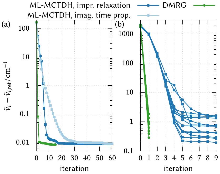
X. نشر SPFs غير المشغولة وإثراء الفضاء الفرعي

هنا، سنناقش كيفية التعامل مع نشر SPFs غير المشغولة غير المحددة وكيفية توسيع أو “إثراء” الفضاء الفرعي لـ SPF. كلا الموضوعين مرتبطان ببعضهما البعض وقد كانت الأبحاث حول هذه الموضوعات نشطة جدًا مؤخرًا في مجتمعات MCTDH و DMRG.

A. نشر SPFs غير المشغولة

في معظم السيناريوهات، يزداد عدد SPFs المطلوبة (أبعاد الربط لـ TTNS) مع مرور الوقت. تبدأ العديد من المحاكاة حتى بحالة هارتري واحدة كحالة أولية (SPF واحدة فقط مشغولة في كل بعد، )، وبعد بضع خطوات زمنية، يمكن أن تصبح الحالة مرتبطة بسرعة. لأخذ ذلك في الاعتبار، يجب على المرء إما استخدام TTNS أولية بأبعاد ربط أكبر (SPFs غير مشغولة إضافية في البداية)، أو يجب على المرء إضافة SPFs ديناميكيًا خلال تطور الزمن. الحالة الأولى هي الحالة الافتراضية في MCTDH، والثانية هي تطوير حديث [106، 176، 177]. في كلتا الحالتين، تصبح مصفوفة كثافة الجسيمات الفردية التي تحتاج إلى أن تُعكس في معادلات حركة SPF، المعادلة (19)، مفردة (تختفي الشغلات الطبيعية). لتجنب المصفوفات المفردة، يتم تنظيمها عمليًا خلال نشر الزمن [2]. بالنسبة للعديد من التطبيقات النموذجية، تعمل التنظيم بشكل جيد. هذه هي الحالة حتى عند استخدام مساحات SPF غير المباشرة وإضافة وإزالة SPFs جديدة خلال المحاكاة [106]. بدلاً من عكس مصفوفة الكثافة، يمكن للمرء عكس معامل التنسور المنظم، مما يؤدي إلى تحسين الاستقرار . ومع ذلك، حتى مع تحسين الاستقرار، يمكن أن تصبح التنظيم مشكلة من حيث الاستقرار العددي والكفاءة العددية [99، 129، 178، 179].
رسميًا، في TDVP-DMRG لا يوجد عكس لمصفوفة الجسيم الفردي المعنية، ولا يتطلب أي تنظيم صريح. بينما تعتبر طريقة TDVP-DMRG قوية بالنسبة للشغلات الطبيعية الصغيرة [142]، فإن تقويم SHFs غير محدد بالنسبة للمصفوفات الكثافة المفردة، وبالتالي تصبح أي إجراء تقويم أيضًا عشوائيًا. ومع ذلك، فإن الحجج التي تقول إنه لا يمكن نشر SPFs غير المشغولة في TDVP-DMRG [149] لا تصمد، حيث يمكن للمرء دائمًا تعديل SPFs غير المشغولة بشكل مناسب، على سبيل المثال، إما باستخدام الإجراءات الموصوفة في القسم X B أو حتى باستخدام طريقة التنظيم القياسية في MCTDH.
بشكل عام، يمكن أن تصف الطرق التي تستخدم TDVP SPFs فقط من الدرجة الأولى في الزمن وبالتالي هناك دائمًا عشوائية فيما يتعلق بـ SPFs غير المشغولة [129]. هذا ينطبق على (ML-)MCTDH و TDVP-DMRG، بغض النظر عن الطريقة التي يتم بها التنظيم (أو ما إذا كانت “مخفية” باستخدام تحلل المصفوفات أو المقاييس [76]). وبالتالي، في سيناريوهات معينة، يجب توخي الحذر لضمان تقارب المحاكاة بشكل صحيح [76، 179، 180]، على الرغم من أن التنظيم القياسي يعمل بشكل جيد للعديد من حالات الاستخدام.

B. توسيع الفضاء الفرعي: تحسين SPFs غير المشغولة

بدلاً من محاولة نشر SPFs غير المشغولة، والتي هي غير محددة، يمكن للمرء بدلاً من ذلك تحسينها بشكل مختلف. هناك طرق مختلفة لتحسين SPFs غير المشغولة، والتي تُعرف أيضًا في لغة DMRG بإثراء الفضاء الفرعي أو توسيع الفضاء الفرعي. هنا، سنناقش أولاً نهج DMRG ذو الموقعين، ثم نتابع مع نهج MCTDH، وأخيرًا نناقش نهج DMRG ذو الموقع الواحد. العديد من هذه مرتبطة ببعضها البعض.
الشكل 31. هاميلتونيان فعال ذو موقعين. يتم استخدام TTNS من الشكل 5 كمثال. يؤدي تشخيص الهاميلتونيان الفعال إلى تحسين التنسور المعروض في المستطيل المنقط، وهو انكماش لـ مع . المستطيل الرمادي يتوافق مع الهاميلتونيان . قارن مع المعادلة (49).

1. نهج DMRG ذو الموقعين

في الممارسة العملية، يتم تخفيف بعض ولكن ليس كل القضايا المحتملة الناشئة عن الوصف من الدرجة الأولى لـ SPFs في TDVPDMRG باستخدام ما يسمى خوارزمية الموقعين، حيث يتم حل مشكلة النشر المحلية في الفضاء الفرعي ليس لتنسور واحد ولكن لتنسورين في الشجرة. يتم ذلك عن طريق أولاً انكماش التنسور الجذري وأحد جيرانه، ثم نشر التنسور المنكمش، وأخيرًا “فك انكماش” التنسور المنشر باستخدام، على سبيل المثال، SVD. في لغة MCTDH، نعرف تكوينات SHF على أنها
حيث تحتوي على جميع المؤشرات ولكن . ثم يحل DMRG ذو الموقعين معادلة شرودنجر في فضاء تكوينات SHF و SPF، وبالتالي يقوم DMRG ذو الموقعين بشكل فعال بتحسين زوج من معامل التنسور SHF-SPF. يؤدي ذلك إلى هاميلتونيان فعال مع عناصر مصفوفة
قارن مع الشكل 31.
يمكن أن يتجنب المتغير ذو الموقعين مشاكل التقارب وهو مهم بشكل خاص لـ DMRG المتكيف مع التناظر [35]. قبل أن يتمكن المرء من تقويم العقدة التالية في المسح، يجب فك انكماش التنسور ذو الموقعين باستخدام، على سبيل المثال، SVD. وهذا يسمح بطريقة مباشرة لضبط أبعاد الربط ديناميكيًا (عدد SPFs). من خلال ملاحظة مجموع القيم المفردة المهملة، يحصل المرء على تقدير للخطأ، والذي يمكن استخدامه لتقديرات الطاقة [7، 181، 182]. في الواقع، تم صياغة DMRG القياسي في البداية كخوارزمية ذات موقعين [3] والإصدار ذو الموقع الواحد هو تطوير أكثر حداثة [183]. ومع ذلك، لاحظ أن TDVP-DMRG ذو الموقعين لا يزال يعتمد على TDVP وبالتالي قد لا يتم حل القضايا المحتملة بسبب SPFs غير المشغولة بالكامل. يُعرف DMRG ذو الموقعين أيضًا باسم ALS المعدل [168].

2. نهج لي/فيشر/مانث

تطوير خوارزميات لتوسيع مساحة SPF/أبعاد الربط بشكل منهجي هو أمر مباشر، وكلا من MCTDH و TDVP-DMRG ذو الموقع الواحد تم تطوير العديد من المخططات لزيادة عدد SPFs/أبعاد الربط ديناميكيًا خلال الزمن [69، 106، 150، 176، 177، 184، 185]. من الصعب أكثر فعلاً تحسين SPFs الجديدة المضافة وبالتالي غير المشغولة. لتحسين SPFs غير المشغولة/لتوسيع الفضاء الفرعي، تم تطوير نهج مختلفة في مجتمعات DMRG و MCTDH. نناقش أولاً الحلول المطورة في سياق MCTDH. هناك، الفكرة العامة هي أنه بدلاً من نشر SPFs التي تكون غير مشغولة في الوقت ، والتي هي غير محددة، يتم تحسينها من خلال تعظيم كمية تتعلق بالتداخل بين SPFs المشغولة في ذلك الوقت . وهذا يسمح بتوسع طبيعي لمساحة SPF خلال تطور الزمن. يمكن اشتقاق مثل هذا التعبير بطرق مختلفة، لكن الشكل العام للتعبير المستمد من قبل علماء مختلفين متشابه.
استمد لي وفيشر تعبيرًا عن SPFs المثلى لـ MCTDH البوزوني [15، 186، 187] من خلال تقليل الخطأ [188]. استمد مانث نفس التعبير بلغة MCTDH العادية (ML-) من خلال تحليل توسع مصفوفة كثافة الجسيم الفردي إلى الدرجة الثانية في الزمن [129، 189]. لتحليل التعبير الذي توصل إليه مانث، نعتبر هنا فقط SHFs الطبيعية، المشار إليها بـ من خلال فحص الشغلات الطبيعية، نقسم SHFs
الشكل 32. عامل مرتبط بـ SPFs غير المشغولة المثلى. قارن مع المعادلة (50). يتم استخدام TTNS من الشكل 5 كمثال. المستطيل الرمادي يتوافق مع الهاميلتونيان والمربع الأزرق يتوافق مع عكس الشغلات الطبيعية (تداخلات SHFs الطبيعية). المنطقة المخططة باللون الأزرق تتوافق مع التقريب المقدم في المعادلة (56). هذا يتجنب حساب في فضاء الأساس البدائي.
و SPFs المقابلة في المشغولة ( occ) وغير المشغولة. لاحظ أن هذا يقدم معلمة عددية. التعبير المستخدم للعثور على SPFs غير المشغولة المثلى يحتوي بعد ذلك على العامل التالي الممثل بالتكوينات :
حيث يوجه إلى فضاء SHFs الطبيعية المشغولة:
ثم يتم تحديد أفضل SPFs غير المشغولة بواسطة الحالات الذاتية ذات أكبر قيمة ذاتية للمشغل
حيث يتم إسقاطها على SPFs الطبيعية المشغولة. نظرًا لأن تحتوي على كل من و ، فإنها تغطي الفضاء الذي لا يتضمنه الفضاء المماس. يمكن حساب الحالات الذاتية بكفاءة باستخدام حلول القيم الذاتية التكرارية مثل حل لانكزوس. انظر الشكل 32 للحصول على مثال توضيحي.
بينما تحتوي المعادلة (52) على SPFs غير المشغولة التي تكون مثالية من الدرجة الثانية في الزمن، فإن المصطلح في المعادلة (50) مكلف في الحساب لأنه يحتوي على تم تقييمه جزئيًا في الأساس البدائي. بالنسبة لمشغلات SoP (وبالمثل لمشغلات MPOs)، يمكن التعبير عن باستخدام التقسيم من المعادلة (25) كـ
إدخال توسيع SHF-SPF المعادلة (8) يؤدي إلى
التي تحتوي على مجموع مزدوج على جميع المصطلحات في هاملتونيان SoP. لتجنب زيادة ، يمكن تقريب المعادلة (54) من خلال تضمين فقط المصطلحات “القطرية” مع ، مما يؤدي بعد ذلك إلى تنفيذ يتناسب بشكل ملائم. أظهر مانث أن هذا التقريب يؤدي إلى SPFs غير مشغولة مثالية بشكل كافٍ [189].
الشكل 33. الحالة المستخدمة للعثور على SPFs غير مشغولة مثالية بناءً على المعادلتين (55) و(56). قارن مع الشكلين 31 و32.

3. نهج منديف-تابيا/ماير

باستخدام اشتقاق مختلف، توصل منديف-تابيا وماير إلى تعبير عن معاملات SPFs غير المشغولة المثالية [177]. كما اشتقوا تعبيرًا عن SPFs غير المشغولة المثالية التي تتطابق مع المعادلة (50) باستثناء المكلفة، والتي يتم تقريبها من خلال إسقاط هذا التعبير على تكوينات SHFs. يؤدي ذلك إلى تنفيذ فعال لتقريب لـ . باستخدام اشتقاق آخر يشبه أكثر اشتقاق لي وفيشر [188]، توصل مارتينازو وبورغارت إلى نفس التعبير تقريبًا [190].
نظهر الآن أن خوارزمية TDVP-DMRG ذات الموقعين تتعلق بالتعبير من منديف-تابيا وماير. كان اشتقاقهم لمتوسط MCTDH العادي، ولكن يمكن توسيعه بسهولة إلى ML-MCTDH. باستخدام تكوينات SHF، المعادلة (48)، يمكننا تعريف الحالة التالية
ثم من المعادلة (50) المسقطة على فضاء تكوينات SHF، والتي تُسمى هنا يمكن كتابتها كـ
بطريقة مشابهة، من خلال إسقاط على ( ) يمكننا الحصول على تعبير لـ . كيف يرتبط هذا بخوارزمية الموقعين؟ المستخدمة في المعادلة (55) تحتوي على كل من تكوينات SHF وتكوينات SPF المقابلة. يتم الحصول على SHFs وSPFs نفسها من خلال الانكماش مع موتر المعاملات. لذا، يتطلب الأمر موترين للمعاملات لاسترجاع TTNS الكلي من ، والتي تصف وفقًا لذلك التكوينات المستخدمة في خوارزمية DMRG ذات الموقعين! يمكن رؤية ذلك بسهولة من خلال مقارنة الشكل 33، حيث يتم تصوير ، مع هاملتونيان فعال ذو موقعين المقابل الموضح في الشكل 31. لاحظ أن التكلفة الحسابية لاستخدام المعادلة (56) أقل من تلك الخاصة باستخدام خوارزمية DMRG ذات الموقعين حيث يتم انكماش التكوينات في عقدة واحدة في المعادلة (56). لذا، يمكن تفسير التعبير الذي وجده منديف-تابيا وماير كتقريب لخوارزمية DMRG ذات الموقعين، ويمكن استخدام هذا أو تعبيرات مانث ليس فقط في ML-MCTDH ولكن أيضًا في DMRG ذات الموقع الواحد لزيادة مساحة SPF (وبالتالي زيادة أبعاد الربط). لاحظ أن هذه التعبيرات يمكن استخدامها لكل من الانتشار الزمني التخييلي والزمني الحقيقي، وبالتالي يمكن دمجها مع كل من DMRG وTDVP-DMRG.

4. نهج DMRG ذو الموقع الواحد

نناقش الآن الحلول لتجنب التعامل مع قضية انتشار SPFs غير المشغولة التي تم تطويرها في سياق DMRG. اقترح يانغ ووايت توسيع TNS باستخدام انتشار لانكزوس العالمي الإضافي التقريبي [192]، حيث يعمل بشكل صريح (ولكن تقريبي) على . نهج آخر، أكثر شيوعًا بدأه وايت يعتمد على إزعاج الحالة أثناء عملية DMRG [183]. هناك، نقطة البداية مختلفة قليلاً عن تلك الخاصة بـ MCTDH. بينما يتم
توسيع SPFs مباشرة باستخدام القيم الذاتية لـ من المعادلة (52)، في سياق DMRG يحدث ذلك في تمثيل SHF من خلال إضافة بعض الحالات الجديدة إلى فضاء SHF وتعديل إجراء التعميم SHF-SPF. يمكن القيام بذلك إما عن طريق إضافة صفوف إلى موتر المعاملات المصفوفة مع إدخالات تمثل SHF [193]، أو من خلال إنشاء مصفوفة كثافة SHF وإزعاجها باستخدام [183]
لاحظ أن يمثل فضاء SHF وليس هو نفسه مصفوفة كثافة الجسيم الواحد. كلا الإجراءين، إضافة صفوف إلى أو إزعاج ، متطابقان ولكن لهما مقاييس حسابية مختلفة [59، 193]. بجانب الفرق أن فضاء SHF وليس فضاء SPF هو الذي يتم توسيعه، فإن الفرق الرئيسي الآخر عن مخططات توسيع تحت مساحة MCTDH هو أن مخططات DMRG المستقلة عن الزمن قد تشمل ضغطًا إضافيًا للحالة الجديدة مع إلى العدد الأصلي من SPFs. يغير هذا الضغط ، ومن هنا جاء اسم إثراء تحت المساحة. يتم استخدامه لتجنب الحد الأدنى المحلي مع تماثيل غير مرغوب فيها في DMRG.

5. نهج وايت

أكثر مخططات الإثراء استخدامًا في DMRG هو الذي طوره وايت [183]. يعتمد على المعادلة (57) ولكنه تم توسيعه أيضًا إلى إثراء قائم على SVD [193]. لجعل الاتصال بمخططات توسيع MCTDH أكثر وضوحًا، سنقوم بتبادل SPFs وSHFs في ما يلي (أو بشكل مكافئ، النظام والبيئة في لغة DMRG). وبالتالي، لن نزعج مصفوفة كثافة SHF، المعادلة (57) بل سنقوم بقطر مشغل SPF المعادلة (52). في هذا التمثيل، باستخدام نظرية الاضطراب من الدرجة الأولى وأخذًا في الاعتبار تحليل SHF-SPF لهاملتونيان، المعادلة (25)، اشتق وايت المصطلح التالي، الذي نعرضه هنا في تدوين MCTDH:
حيث يتوافق مع الطاقات لكل مصطلح مجموع يتم تقييمه في أساس SPF، وحيث
لاحظ أنه بخلاف ، وتبادل SPFs وSHFs في التعبير الأصلي لوايت (الذي لا نعرضه هنا)، فإن المعادلة (58) تتطابق مع التعبير الذي اشتقه مانث، قارن مع المعادلتين (50) و(54) (حيث غير مدرج). بالنسبة لمشغلات SoP أو، بشكل مكافئ، لمشغلات MPOs مع المصطلحات، تجنب مانث زيادة عن طريق تقييم الجزء من المعادلة (59) بدقة ولكن فقط اعتبار المصطلحات مع للجزء . قام وايت بعمل تقريب أكثر حدة واعتبر . ثم تقيم المعادلة (58) إلى
مع . بدلاً من تقييم بشكل صريح، قام وايت بتعيينها إلى معلمة تجريبية لا تعتمد على . تعتبر التقريبات الأكثر حدة التي قام بها وايت مفيدة حيث اعتبر وايت DMRG المستقل عن الزمن وكان يسعى لإيجاد وسيلة للتغلب على الحد الأدنى المحلي وتحسين التقارب.

6. نهج تباين الطاقة

تم تطوير طرق توسيع تحت المساحة ذات صلة تعتمد على تقليل المساهمة ذات الموقعين في تباين الطاقة [194، 195]،
حيث تسقط على الفضاء الذي يتعامد على الفضاء المماس ذو الموقعين (تم تضمين المساهمات ذات الموقعين والصفر بالفعل في DMRG ذات الموقع الواحد) [154، 194]. بينما تؤدي المعادلة (61) إلى اشتقاق مختلف تمامًا للعثور على SPFs غير مشغولة مثالية، فإن هذا، في الأساس، هو نفس النهج الذي اتبعه منديف-تابيا وماير، المعادلة (56). تستخدم خطة حديثة لتقريب المعادلة (61) بكفاءة تسلسلات من SVDs [196، 197].

7. نهج مُدمج BUG

تمديد لمُدمج BUG غير الحافظ للطاقة [156]، الذي ذكرناه بإيجاز في القسم الثامن، يسمح أيضًا بتمديد تحت المساحة وهو محافظ على النور والطاقة [198، 199]. هناك، يتم زيادة مساحة SPF في الوقت بواسطة تلك في الوقت ويمكن زيادة أبعاد الربط بمقدار يصل إلى عاملين في كل خطوة زمنية. لقد تم توسيعه مؤخرًا من تنسيق تاكر إلى TTNSs [200].

XI. هياكل الشجرة

هنا، سنناقش لماذا تُستخدم TTNSs عادةً لمحاكاة الديناميات الكمومية الجزيئية (الاهتزازية) بينما تُستخدم MPSs وليس TTNSs في معظم المجالات الأخرى. نظرًا لأن هذه المناقشة تعتمد على المشكلة الكمومية، فإننا نقيد مقارنتنا بالأنظمة الجزيئية ونقارن بين الهيكل الإلكتروني الجزيئي والديناميات الاهتزازية الجزيئية. بالإضافة إلى ذلك، وذات صلة بذلك، سنناقش بعض الاستراتيجيات للعثور على هياكل شجرية مثالية لـ TTNSs.

A. TTNSs أم MPSs؟

بالمقارنة مع MPSs، يمكن لـ TTNSs التقاط مجموعات مختلفة من درجات الحرية المرتبطة بكفاءة أكبر وفصلها بكفاءة عن درجات الحرية الأقل ارتباطًا. تتوافق هذه درجات الحرية مع إما المدارات في نظرية الهيكل الإلكتروني أو أوضاع/إحداثيات الاهتزاز (والدوران) في الديناميات الكمومية الاهتزازية. على سبيل المثال، يمكن عادةً وصف تفاعل ما بواسطة بعض أوضاع التفاعل التي تكون مرتبطة بشدة، وبعض الأوضاع “المراقبة” أو “الحمام” التي لا تشارك بشكل مباشر في التفاعل. تسمح TTNSs بفصل كفء لهذه المجموعات من الأوضاع المرتبطة أو غير المرتبطة. بالمقارنة مع MPSs، فإن TTNSs غالبًا ما تتقارب بشكل أسرع فيما يتعلق بعدد SPFs المطلوبة، ، سواء في الديناميات الاهتزازية [59] وفي الهيكل الإلكتروني الجزيئي [26،37،40،201،202]. إذا كان هذا هو الحال، فلماذا نادرًا ما تستخدم TTNSs لمحاكاة الهيكل الإلكتروني؟ السبب هو اختلاف في قياس الحسابات. تحتوي MPSs على موترات بحجم تُوصف MPSs التي تصف الهياكل الإلكترونية بشكل أكثر كفاءة في فضاء Fock [26]. الأبعاد الفيزيائية هي إذن وبالتالي فهي غير ملحوظة. وبالتالي، فإن كل عملية موتر هيكل إلكتروني MPS تتوسع على الأقل كما هو حيث يتراوح من 500 إلى حتى 30,000 [182، 203، 204]. بالمقابل، تتوسع موترات TTNS على الأقل كما هو حيث أن الحد الأدنى من “البعد المفيد” للموتر في الشجرة هو 3. وبناءً عليه، فإن قياس عمليات TTNS في الهيكل الإلكتروني هو عامل أكبر من ذلك الخاص بـ MPSs [201، 202]. حتى إذا كانت TTNSs تتطلب أصغر للتقارب، فإن MPSs بشكل عام أكثر فائدة حسابيًا في العديد من حالات الهيكل الإلكتروني. قد يتغير هذا إذا كان يمكن أيضًا استغلال هيكل الشجرة للهميلتوني (باستخدام TTNO وليس MPO)، مع ضغط عددي للمشغل [135، 205]. ينطبق نفس حجة القياس على استخدام دمج الأوضاع لمحاكاة الهيكل الإلكتروني، والتي يمكن أن تكون مفيدة فقط في حالات خاصة [68، 139].
بالمقابل، يتم إجراء محاكاة الديناميات الاهتزازية في أغلب الأحيان في فضاء هيلبرت، وهناك تكون الأبعاد الفيزيائية من نفس الحجم تقريبًا ثم لا تنطبق الحجة أعلاه بعد الآن وغالبًا ما تقدم TTNSs ميزة حسابية واضحة على MPSs. تم التحقق من ذلك عدديًا في المرجع [59] وتمت ملاحظة تقليل أحجام الموترات وتقليل وقت الحساب عند استخدام TTNSs بدلاً من MPSs لنظام الأسيتونيتريل الاهتزازي ذي الأبعاد 12. لاحظ أن الديناميات الاهتزازية يمكن أيضًا أن تُجرى في فضاء Fock [206-208] ويمكن أن تصف MPSs الديناميات الاهتزازية بكفاءة أيضًا [62-66، 69، 71]. لاحظ أيضًا أن أصغر بكثير مما هو عليه في محاكاة الهيكل الإلكتروني الجزيئي النموذجية. على سبيل المثال، استخدمت محاكاة لدينا على نظام زوندل للحصول على حالات مثارة اهتزازية مع خطأ في الطاقة قدره [70]. على الرغم من “صغر” بالمقارنة مع الهيكل الإلكتروني، من حيث هذا هو أحد أكبر محاكاة TTNS/ML-MCTDH الاهتزازية التي تمت على أنظمة غير نموذجية واقعية. العديد من التطبيقات لا تتطلب مثل هذا التقارب الطاقي الضيق (على سبيل المثال، حيث تكون الملاحظات الأخرى ذات أهمية) وبالتالي تتطلب أصغر. التحدي الحسابي هو إذن مختلف ويكمن في المحاكاة الفعالة لتطور الزمن أو حساب العديد من الحالات المثارة، والمعالجة المتقدمة للحصول على الملاحظات المطلوبة، وإعداد هميلتوني واقعي [13، 209-212].

ب. هيكل الشجرة الأمثل

تعتمد كفاءة MPSs على ترتيب درجات الحرية في MPS. يجب وضع درجات الحرية المرتبطة بشدة بالقرب من بعضها في MPS. نظرًا لإنشاء العديد من الخوارزميات المتطورة باستخدام أساليب التحسين العالمية ورؤى من نظرية المعلومات الكمومية [7، 182، 213-215]، يمكن اعتبار هذه المشكلة غير البسيطة في التحسين قد تم حلها.
تم تكريس اهتمام أقل لتحسين هياكل الأشجار، وهو أمر أكثر تعقيدًا. أحد المبادئ التوجيهية الرئيسية لإعداد شجرة فعالة هو أن البعد الأمثل للموتر هو ثلاثة [21،37،59،201،202]. يمكن التعبير عن أي هيكل شجرة باستخدام موترات ثلاثية الأبعاد وتقييد أبعاد الموترات إلى ثلاثة يسمح بتطوير أسهل للبرامج [202]. لماذا استخدام موترات ثلاثية الأبعاد وليس موترات ذات أبعاد أعلى؟ يتوسع حجم كل موتر مع حيث أن هو البعد. تتوسع تطبيقات مشغلات SoP على موتر كما هو . وبالتالي، كلما زاد بعد الموتر، زادت سوء القياس! يجب استخدام أقل بعد ممكن للموتر لا يزال يسمح بإنشاء الأشجار، وهو ثلاثة. تُستخدم أحيانًا موترات ثنائية الأبعاد في تطبيقات ML-MCTDH (بما في ذلك مثالنا في الشكل 5)، لكنها لا يمكن أن تعبر عن تفرع الشجرة، ويمكن تقييدها لتكون قطرية [126،216]، أو يمكن امتصاصها في موتر مجاور، كما هو الحال بالنسبة لمصفوفة في عمليات DMRG (انظر الشكل 28).
إذا كانت الموترات ثلاثية الأبعاد هي الأكثر مثالية ويجب تجنب الموترات ثنائية الأبعاد للحصول على TTNSs بأفضل قياس فيما يتعلق بعدد المعلمات، فلماذا يتم استخدام أبعاد موتر غير مثالية على ما يبدو في تطبيقات ML-MCTDH الفعلية؟ نحن غير مدركين أن هذا قد تم مناقشته في أدبيات ML-MCTDH ونقدم هنا ثلاثة إجابات محتملة. (1) أحد الأسباب العملية هو أن دمج الأوضاع يؤدي على الفور إلى موترات عالية الأبعاد. بالنسبة للأنظمة النموذجية، يمكن تجنب دمج الأوضاع، ولكن بالنسبة للأنظمة غير النموذجية، فإن دمج الأوضاع أمر حاسم لتناسب الإمكانات بشكل مثالي في شكل SoP [211، 217، 218]. (2) سبب آخر، أكثر تكهنًا، هو أن الموترات ذات الأبعاد الأعلى تسمح بوجود “اتصال” أقرب للمجموعات المرتبطة بشدة. يؤدي استخدام الموترات ثلاثية الأبعاد فقط إلى المزيد من الطبقات والمزيد من الموترات في الشجرة. بينما لم نلاحظ صعوبات عددية باستخدام خوارزميات DMRG، قد تؤدي العديد من الموترات والطبقات في TTNS إلى صعوبات عند دمج معادلات الحركة ML-MCTDH. (3) تؤدي الأشجار ذات الطبقات العديدة إلى عيوب حسابية عند استخدام التكامل لتقييم مشغل الإمكانات في ML-MCTDH [19]، على الرغم من أن التطورات الأخيرة قد حسنت من ذلك [219]. وبالتالي، بينما قد تعطي الموترات ثلاثية الأبعاد أفضل قياس فيما يتعلق بعدد المعلمات وتطبيقات المشغل، هناك أسباب أخرى لا تسمح باستخدام الموترات ثلاثية الأبعاد فقط. هناك حاجة إلى مزيد من الدراسات لتوضيح ذلك.
تحسين هيكل الشجرة صعب بالنسبة للأنظمة غير النمذجة (وأحيانًا حتى للأنظمة النمذجة) وفي تطبيقات ML-MCTDH النموذجية، يتم توجيه إعداد هيكل الشجرة في الغالب بواسطة الحدس الكيميائي والتجربة والخطأ. لتحسين ذلك، قدمنا طريقة منهجية وآلية للعثور على الشجرة المثلى بناءً على بعض التخمينات الأولية، أي أن الشجرة الأولية غير المحسّنة تُفكك إلى شجرة أكثر مثالية حيث يتم فصل درجات الحرية المرتبطة وغير المرتبطة بشكل أفضل عن بعضها البعض. كما هو الحال في ترتيب MPS، هذه مشكلة صعبة من نوع NP ويجب استخدام طرق تحسين هيوريستية. كانت طريقتنا في “فك الارتباط” تعتمد في البداية على نهج جشع وتحتوي على أربع خطوات: (1) يتم اختيار موتر وجاره بشكل عشوائي، ويتم دمجهما، وتعيينهما كعقدة جذر جديدة. (2) ثم يتم إزعاج أبعاد موتر الموقعين الناتجين بشكل عشوائي. (3) عند تقسيم ثنائي مختار عشوائيًا، يتم “فك انكماش” موتر الموقعين باستخدام SVD. (4) يتم الاحتفاظ بالموترين الناتجين كلما كان حجم الزوج الناتج من الموترات أصغر من حجم الزوج الأولي من الموترات. تتكرر هذه الخطوات الأربع طالما كان هناك تقليل كبير في العدد الإجمالي للمعلمات. تؤدي هذه العملية البسيطة ولكن السريعة إلى نتائج جيدة جدًا، وتمكنا من العثور على هيكل شجرة أكثر مثالية لنظام الأسيتونيتريل الاهتزازي ذي الأبعاد 12. مؤخرًا، قمنا بتوسيع نهجنا الجشع إلى التلدين المحاكى، مما يسمح لنا بالتغلب على القيم الدنيا المحلية التي وجدها النهج الجشع. علاوة على ذلك، أضفنا خيار إزالة وإضافة العقد، مما يجعل تحسين هيكل الشجرة هذا عامًا تمامًا.
مثال على تحسين هيكل الشجرة لدينا موضح في الشكل 34 لمشكلة إيجاد شجرة مثالية لأيون إيغن ذي الأبعاد 33 [212،223]. تؤدي إجراءات تحسين الشجرة لدينا إلى TTNS (الشكل 34(b)) الذي يعطي طاقة تبلغ 70 بعدد روابط. أقل من النموذج غير المحسن الموضح في الشكل 34(أ)، الذي تم استخدامه كافتراض أولي وتم أخذه من المرجع [212،223]. حتى مع طاقة الشجرة غير المحسّنة لا تزال أقل من طاقة الشجرة المحسّنة مع ! لاحظ أنه، باستثناء تركيبة الوضع، تحتوي الشجرة غير المحسّنة على موترات رباعية الأبعاد بينما تحتوي الشجرة المحسّنة فقط على موترات ثلاثية الأبعاد، وهو ما يتماشى مع مناقشتنا أعلاه. تتيح لنا إجراءات التحسين لدينا أيضًا الحصول على رؤى حول النظام الجزيئي حيث تحدد الأوضاع المرتبطة بقوة. يمكن استخدام تحسين هيكل الشجرة لكل حالة ذاتية، ويمكن استخدامه أثناء انتشار الزمن من خلال تحسين الهيكل بعد كل بضع خطوات زمنية.
في فيزياء المادة المكثفة، تم اقتراح تحسين هيكل الشجرة ذات الصلة مؤخرًا والتي تعتمد إما على تقسيمات التشابك [224] أو على تحسين الهيكل مشابه لما نقوم به ولكن يتم خلال تحسين DMRG [225]. هذه الإجراءات وإجراءاتنا تعتمد على بعض التخمينات الأولية للشجرة وهاميلتونيان أولي. الأول سهل الحصول عليه ولكن بالنسبة للأخير في الأنظمة غير النموذجية غالبًا ما يحتاج المرء إلى ملاءمة الجهد [211،217،218]، مما يتطلب أحيانًا العثور على تركيبات وضع مثالية. نهج مقترح مؤخرًا للقيام بذلك هو تحليل الارتباطات من محاكاة الديناميكا الجزيئية الكلاسيكية بطرق مشابهة جدًا لأساليب المعلومات الكمومية المستخدمة في DMRG [226]. بدلاً من ذلك، يمكن للمرء أولاً استخدام تركيبة وضع غير مثالية للحصول على ملاءمة جهد غير مثالية ثم استخدام تحسين هيكل الشجرة.
الشكل 34. TTNSs مع هيكل (غير) محسن لأيون الاهتزازات الذاتية ذو الأبعاد 33. (أ) الهيكل الشجري المستخدم في المرجع [212، 223]. (ب) الهيكل المحسن باستخدام الخوارزمية من المرجع [59]. الرموز تشير إلى الإحداثيات المحددة [212]. الأرقام تشير إلى أبعاد الروابط المستخدمة خلال تحسين حالة الأرض DMRG مع عدد متكيف من SPFs مع القيمة القصوى المحددة إلى الطاقة المحسّنة بواسطة DMRG لقيمتين من مُعَروضة في الصناديق الرمادية. لم يتم تحسين تركيبات الوضع (مجموعات الإحداثيات) خلال تحسين هيكل الشجرة، ولكن هذا ممكن.
من خلال فحص أي الأوضاع مجمعة معًا، فإن ذلك يعطي تلقائيًا أيضًا تركيبات أوضاع مثلى.

اثنا عشر. الاستنتاجات

طريقة ML-MCTDH وDMRG هما خوارزميات قوية ذات خلفية رياضية مشتركة، لكن تم تطويرهما في مجتمعات مختلفة وتستخدم لغات مختلفة تمامًا لوصف نفس التعبيرات الرياضية. هنا، قدمنا مقارنة مباشرة وشاملة بين نظريات ML-MCTDH وDMRG من خلال ترجمة تعبيرات MCTDH إلى مخططات الشبكة التنسورية ومقارنة خوارزميات ML-MCTDH وDMRG لحل معادلة شرودنغر.
تتشابه العديد من التطورات المستقلة في مجتمعات ML-MCTDH وDMRG بشكل كبير، ولكن تُستخدم لغات مختلفة وغالبًا ما تُشتق تعبيرات مشابهة بناءً على نهج وسياقات مختلفة. لقد أبرزنا ذلك من خلال إظهار أوجه التشابه بين النظريات المستخدمة في كلا المجالين للموضوع المتقدم المتعلق بإثراء الفضاء الفرعي أو، بشكل مكافئ، إيجاد دوال الجسيم الفردية غير المشغولة المثلى. أخيرًا، ناقشنا لماذا تُستخدم الأشجار بشكل شائع في الديناميات الكمية الجزيئية ولكن لماذا تُفضل MPSs حاليًا في بنية الإلكترون الجزيئية، وكيفية تحسين هياكل الأشجار.
تتمتع “اللغات” الرياضية المختلفة بقوى تعبيرية مختلفة. في رأينا، تعتبر الرسوم البيانية مفيدة بشكل خاص في تسليط الضوء على انقباضات التنسور، وتقدم تمثيلات بصرية ملائمة للمعادلات الرياضية التي يمكن استخدامها أيضًا في الاشتقاقات، كما أظهرنا هنا من خلال اشتقاق معادلات ML-MCTDH. على النقيض من ذلك، نعتقد أن لغة MCTDH مريحة جدًا لتسليط الضوء على الفضاءات الفرعية المختلفة في TTNS والأسس الهرمية. نأمل أن تسهم هذه المساهمة في تعزيز استخدام الرسوم البيانية في أدبيات MCTDH وكذلك استخدام مفاهيم MCTDH في أدبيات DMRG.
لم يتم تناول العديد من المواضيع هنا، وقد أغفلنا بعض التطورات في الرياضيات التطبيقية، بالإضافة إلى البدائل لطريقة ML-MCTDH وDMRG. على سبيل المثال، المواضيع الأخرى التي تم تناولها من قبل كلا المجتمعين ولكننا لم نناقشها هنا تتعلق بتمثيل الشبكة التنسورية لهاملتونيان وكيفية حساب الجسيمات القابلة للتمييز، ومصفوفات الكثافة ودرجة الحرارة المحدودة. نظرًا لأن طريقة ML-MCTDH وDMRG تُستخدم عادةً في مجالات بحث مختلفة، فإن بعض المواضيع تتطور بشكل أكثر نشاطًا من قبل أحد المجتمعين المعنيين. على سبيل المثال، المواضيع
التي تُستخدم بشكل أكثر نشاطًا في طرق MCTDH هي التقليم (اختيار التكوين) وتمثيلات الشبكة ذات الأساس المختلط. وعلى العكس، فإن المواضيع التي تُستخدم بشكل أكثر نشاطًا في سياق DMRG هي التماثلات، وحسابات الطيف في مجال التردد، والنهج العالمية التي تطبق مباشرة الهاميلتوني على شبكة الموتر. بالنظر إلى هذه الأمثلة، لا يزال هناك مجال كبير لتبادل الأفكار بشكل متبادل. نأمل أن يساعد هذا المقال في تعزيز المزيد من تبادل المعرفة الذي سيساهم في تقدم الموضوع الشامل لحالات شبكة الموتر.

شكر وتقدير

تشكر H.R.L. A. M. Nierenberg على المناقشات المفيدة، وأوفي مانثي، هانس-ديتر ماير، وإمام وايهوتمه على التعليقات حول النسخة الأولية من هذه المقالة.

تمويل

تم دعم هذا العمل من قبل مؤسسة العلوم الوطنية الأمريكية (NSF) عبر منحة رقم CHE-2312005. جاء دعم إضافي من تمويل بدء التشغيل بجامعة كاليفورنيا في ميرسيد، ومن خلال الوقت الحاسوبي على مجموعات بيناكلز وميرسيد في جامعة كاليفورنيا في ميرسيد (المدعومة من NSF OAC-2019144 وACI-1429783).
[1] هـ. د. ماير، أ. مانث، و ل. س. سيدر باوم، نهج هارتري متعدد التكوينات المعتمد على الزمن، رسائل الكيمياء والفيزياء 165، 73 (1990).
[2] U. Manthe، H.-D. Meyer، و L. S. Cederbaum، ديناميات حزمة الموجات ضمن إطار هارتري متعدد التكوينات: الجوانب العامة والتطبيق على NOCl، J. Chem. Phys. 97، 3199 (1992).
[3] س. ر. وايت، صيغة مصفوفة الكثافة لمجموعات إعادة التعيين الكمية، فيزيكال ريفيو ليترز 69، 2863 (1992).
[4] س. ر. وايت، خوارزميات مصفوفة الكثافة لمجموعات إعادة التدوير الكمومية، فيزي. ريف. ب 48، 10345 (1993).
[5] س. ر. وايت و ر. ل. مارتن، كيمياء الكم الأولية باستخدام مجموعة إعادة تنظيم مصفوفة الكثافة، J. Chem. Phys. 110، 4127 (1999).
[6] أ. أ. ميتروشينكوف، ج. فانو، ف. أورطولاني، ر. لينغويري، و ب. بالمييري، الكيمياء الكمومية باستخدام مجموعة إعادة تنظيم مصفوفة الكثافة، مجلة الكيمياء الفيزيائية 115، 6815 (2001).
[7] ج. ك.-ل. تشان و م. هيد-غوردون، حسابات ذات ارتباط عالٍ باستخدام خوارزمية بتكلفة متعددة الحدود: دراسة لمجموعة إعادة تطبيع مصفوفة الكثافة، مجلة الكيمياء الفيزيائية 116، 4462 (2002).
[8] Ö. ليغيزا، ج. رودر، و ب. أ. هيس، دراسة QC-DMRG لتقاطع المنحنى الأيوني-المحايد لـ LiF، فيزيائيات الجزيئات 101، 2019 (2003)، arxiv:condmat/0208187.
[9] ج. زانغيليني، م. كيتزلر، س. فابيان، ت. برافك، وأ. سكرينزي، نهج MCTDHF لديناميات الإلكترونات المتعددة في مجالات الليزر، فيزياء الليزر. 13، 6 (2003).
[10] ت. كاتو و هـ. كونو، نظرية التعددية الزمنية المعتمدة على الزمن لديناميات الإلكترونات في الجزيئات في حقل ليزر مكثف، كيمياء. فيزيكس. رسائل 392، 533 (2004).
[11] م. نيست، ت. كلمروث، و ب. سالفرانك، طريقة هارتري-فوك متعددة التكوينات المعتمدة على الزمن للحسابات الكيميائية الكمومية، مجلة الكيمياء الفيزيائية 122، 124102 (2005).
[12] ج. كايلات، ج. زانغيليني، م. كيتزلر، أ. كوتش، و. كراوزر، و أ. سكرينزي، أنظمة متعددة الإلكترونات المترابطة في مجالات الليزر القوية: نهج هارتري-فوك متعدد التكوينات المعتمد على الزمن، فيزي. ريف. أ 71، 012712 (2005).
[13] ه.-د. ماير، ف. غاتي، و ج. أ. وورث، محررون، الديناميات الكمومية متعددة الأبعاد: نظرية MCTDH وتطبيقاتها، الطبعة الأولى. (وايلي-فيتش، فاينهايم، 2009).
[14] د. هوشتول، ج. م. هينز، وم. بونيتز، طرق متعددة التكوين تعتمد على الزمن لمحاكاة العمليات الضوئية لأشعة الإلكترونات في الذرات ذات الإلكترونات المتعددة، المجلة الأوروبية للفيزياء: الموضوعات الخاصة 223، 177 (2014).
[15] أ. ي. ج. لود، س. ليفيك، ل. ب. مادسن، أ. إ. ستريلتسوف، وأ. إ. ألون، ندوة: طرق هارتري متعددة التكوين تعتمد على الزمن للجسيمات غير القابلة للتمييز، مراجعة الفيزياء الحديثة 92، 011001 (2020).
[16] ت. ج. كولدا و ب. و. بادير، تحليل الموترات وتطبيقاتها، مراجعة SIAM 51، 455 (2009).
[17] ه.-د. ماير و ج. أ. وورث، الديناميات الجزيئية الكمومية: نشر حزم الموجات ومشغلات الكثافة باستخدام طريقة هارتري متعددة التكوينات المعتمدة على الزمن، الحسابات الكيميائية النظرية 109، 251 (2003).
[18] هـ. وانغ و م. ثوس، صياغة متعددة الطبقات لنظرية هارتري متعددة التكوين المعتمدة على الزمن، مجلة الكيمياء الفيزيائية 119، 1289 (2003).
[19] U. Manthe، نهج هارتري متعدد الطبقات ومتعدد التكوينات المعتمد على الزمن للديناميات الكمومية على أسطح الطاقة المحتملة العامة، مجلة الكيمياء الفيزيائية 128، 164116 (2008).
[20] ر. جوليان، ب. بفيوتي، ج. ن. فيلدز، و س. دونياش، طريقة إعادة التسمية عند درجة حرارة صفر للأنظمة الكمومية. I. نموذج إيسينغ في حقل عرضي في بعد واحد، فيزيكال ريفيو B 18، 3568 (1978).
[21] ي.-ي. شي، ل.-م. دوآن، و ج. فيدال، المحاكاة الكلاسيكية لأنظمة الكم ذات الجسم المتعدد باستخدام شبكة موتر شجرية، فيزيكس ريفيو A 74، 022320 (2006).
[22] و. هاكبوش وس. كوهين، مخطط جديد لتمثيل التنسور، مجلة تحليل فورييه والتطبيقات 15، 706 (2009).
[23] و. هاكبوش، فضاءات التنسور وحساب التنسور العددي، الطبعة الثانية، سلسلة سبرينغر في الرياضيات الحاسوبية، المجلد 56 (سبرينغر، شام، سويسرا، 2019).
[24] ل. غراسي ديك، تحليل القيم الفردية الهرمي للموترات، مجلة SIAM لتحليل المصفوفات والتطبيقات 31، 2029 (2010).
[25] ل. غراسي ديك، د. كريسنر، و ج. توبلر، مسح أدبي لتقنيات تقريب التنسور منخفض الرتبة، ميتل شترايفن غام 36، 53 (2013).
[26] س. سزلاي، م. بففر، ف. مورغ، ج. باركزا، ف. فيرسترات، ر. شنايدر، و أ. ليغيزا، طرق حاصل الضرب التنسوري وتحسين التشابك لـ كيمياء الكم الأولية، المجلة الدولية لكيمياء الكم 115، 1342 (2015).
[27] ج. فيدال، محاكاة فعالة للأنظمة الكمية ذات الجسم الواحد، فيزيكال ريفيو ليترز 93، 040502 (2004).
[28] س. ر. وايت و أ. إ. فيغوين، التطور في الوقت الحقيقي باستخدام مجموعة إعادة تنظيم مصفوفة الكثافة، فيزيكال ريفيو ليترز 93، 076401 (2004).
[29] أ. إ. فيغوين و س. ر. وايت، طرق استهداف خطوة الزمن للديناميات في الوقت الحقيقي باستخدام مجموعة إعادة تشكيل مصفوفة الكثافة، فيزي. ريف. ب 72، 020404 (2005).
[30] س. بايكل، ت. كوهلر، أ. سوبودا، س. ر. مانمانا، أ. شولووك، و ج. هوبغ، طرق تطور الزمن لحالات المنتج المصفوفي، آن. فيز. 411، 167998 (2019).
[31] م. فانس، ب. ناتشرغالي، و ر. ف. ويرنر، حالات مرتبطة نهائيًا على سلاسل سبين الكم، اتصالات. رياضيات. فيزيكس 144، 443 (1992).
[32] س. أستلوند وس. رومر، الحد الديناميكي الحراري لمصفوفة الكثافة المعاد تنظيمها، فيزيكال ريفيو ليترز 75، 3537 (1995).
[33] ج. فيدال، محاكاة كلاسيكية فعالة للحسابات الكمومية المتشابكة قليلاً، فيزيكال ريفيو ليترز 91، 147902 (2003).
[34] ف. فيرسترات وج. إ. سيراك، تمثل حالات المنتج المصفوفي الحالات الأساسية بدقة، فيزيكس ريفيو ب 73، 094423 (2006).
[35] U. Schollwöck، مجموعة إعادة تنظيم مصفوفة الكثافة في عصر حالات منتج المصفوفات، آن. فيز. 326، 96 (2011).
[36] ر. هوبنر، ف. نيبندال، و و. دور، حالات الشبكة التنسيلية المتسلسلة، نيو ج. فيز. 12، 025004 (2010).
[37] V. Murg، F. Verstraete، Ö. Legeza، و R. M. Noack، محاكاة الأنظمة الكمومية المرتبطة بقوة باستخدام شبكات موتر الشجرة، فيزيكال ريفيو B 82، 205105 (2010).
[38] H. J. Changlani، S. Ghosh، C. L. Henley، و A. M. Läuchli، مضاد المغناطيس هايزنبرغ على أشجار كايلي: طيف الطاقة المنخفضة وعدم التوازن في المواقع الزوجية والفردية، فيزيكال ريفيو B 87، 085107 (2013).
[39] م. جيرستر، ب. سيلفي، م. ريتزي، ر. فازيو، ت. كالاركو، و س. مونتانجيرو، شبكة موتر الشجرة غير المقيدة: صورة قياس تكيفية لأداء معزز، فيز. ريف. ب 90، 125154 (2014).
[40] V. Murg، F. Verstraete، R. Schneider، P. R. Nagy، و Ö. Legeza، حالة شبكة موتر الشجرة بترتيب موتر متغير: طريقة متعددة المراجع فعالة للأنظمة المرتبطة بقوة، J. Chem. Theory Comput. 11، 1027 (2015).
[41] ف. فيرسترات وج. إ. سيراك، خوارزميات إعادة التعيين للأنظمة الكمية ذات الجسم المتعدد في بعدين وأبعاد أعلى، arXiv:condmat/0407066 (2004)، arxiv:cond-mat/0407066.
[42] ج. فيدال، إعادة تنظيم التشابك، فيزيكال ريفيو ليترز 99، 220405 (2007).
[43] ج. فيدال، فئة حالات الكوانتم ذات الجسم المتعدد التي يمكن محاكاتها بكفاءة، فيزيكال ريفيو ليترز 101، 110501 (2008).
[44] ف. فيرسترات، م. م. وولف، د. بيريز-غارثيا، وج. إ. سيراك، الحرجية، قانون المساحة، والقوة الحسابية لحالات الأزواج المتشابكة المتوقعة، فيزيكال ريفيو ليترز 96، 220601 (2006).
[45] إتش. جي. تشانغلاني، جي. إم. كيندر، سي. جي. أومريغار، وجي. كيه.-إل. تشان، تقريبات دوال الموجة المرتبطة بقوة باستخدام حالات ناتج المرافقات، فيزيكال ريفيو بي 80، 245116 (2009).
[46] ك. هـ. مارتى، ب. باور، م. رايهر، م. تروير، و ف. فيرسترات، حالات شبكة موتر الرسم البياني الكامل: اقتراح جديد لوظيفة موجية فرميونية للجزيئات، نيو ج. فيز. 12، 103008 (2010).
[47] ج. ك.-ل. تشان، دوال الموجة ذات التشابك المنخفض، وايلي إنتر ديسيبلاين. ريف. كومبيوتر. مول. ساي. 2، 907 (2012).
[48] ر. أورو، مقدمة عملية لشبكات التنسور: حالات المنتج المصفوفي وحالات الزوج المتشابك المتوقعة، آن. فيز. 349، 117 (2014).
[49] ر. هاغشناس، م. ج. أوروك، و ج. ك.-ل. تشان، تحويل حالات الزوج المتشابك المتوقعة إلى شكل قياسي، فيزيكال ريفيو ب 100، 054404 (2019).
[50] م. ب. زالتيل و ف. بولمان، حالات الشبكة التنسورية المتساوية القياس في بعدين، فيزيكال ريفيو ليترز 124، 037201 (2020).
[51] U. Schollwöck، مجموعة إعادة التعيين لمصفوفة الكثافة، مراجعة الفيزياء الحديثة 77، 57 (2005).
[52] ك. أوييدا، ج. جين، ن. شباتا، ي. هيدا، و ت. نيشينو، مبدأ العمل الأقل لمجموعة إعادة تطبيع مصفوفة الكثافة في الزمن الحقيقي، arXiv:0612480 (2006)، arxiv:cond-mat/0612480.
[53] ج. ج. دوراندو، ج. هاكمان، و ج. ك.-ل. تشان، نظرية الاستجابة التحليلية لمجموعة إعادة تنظيم مصفوفة الكثافة، مجلة الكيمياء الفيزيائية 130، 184111 (2009).
[54] ج. هايجيمان، ج. آي. سيراك، ت. ج. أوزبورن، إ. بيزوران، هـ. فيرشيلد، و ف. فيرسترات، مبدأ التباين الزمني للأنظمة الكمومية، فيزيكال ريفيو ليترز 107، 070601 (2011).
[55] ن. ناكاتاني، س. ووتيرز، د. فان نيك، و ج. ك.-ل. تشان، نظرية الاستجابة الخطية لمجموعة إعادة تشكيل مصفوفة الكثافة: خوارزميات فعالة للحالات المثارة المرتبطة بقوة، مجلة الكيمياء الفيزيائية 140، 024108 (2014).
[56] س. ووترز، ن. ناكاتاني، د. فان نيك، و ج. ك.-ل. تشان، نظرية ثولس لحالات المنتج المصفوفي وطرق إعادة تنظيم مصفوفة الكثافة اللاحقة، فيزي. ريف. ب 88، 075122 (2013).
[57] ج. م. كيندر، س. س. رالف، و ج. كين-ليك تشان، تطور الزمن التحليلي، تقريب الطور العشوائي، ودوال غرين لحالات المنتج المصفوفي، في تقدم في الفيزياء الكيميائية، تحرير س. كايس (جون وايلي وأولاده، هوبوكين، نيو جيرسي، الولايات المتحدة الأمريكية، 2014) الطبعة الأولى، الصفحات 179-192.
[58] هـ. وانغ و م. ثوس، الديناميات الكمية الدقيقة عددياً للجسيمات غير القابلة للتمييز: نظرية هارتري متعددة الطبقات متعددة التكوين المعتمدة على الزمن في تمثيل الكوانتization الثاني، مجلة الكيمياء الفيزيائية 131، 024114 (2009).
[59] هـ. ر. لارسون، حساب حالات الاهتزاز الذاتية باستخدام حالات الشبكة التنسورية الشجرية (TTNS)، مجلة الكيمياء الفيزيائية 151، 204102 (2019).
[60] ب. كلوس، د. ر. رايشمان، ور. تيمبيلا، حسابات حالة المنتج المصفوفة متعددة المجموعات تكشف عن إثارات فرانك-كوندون المتنقلة تحت اقتران هولشتاين من النوع القوي، فيزيكال ريفيو ليترز 123، 126601 (2019).
[61] ج. هايجيمان، س. لوبيتش، إ. أوسيليديتس، ب. فانديرايكن، و ف. فيرسترات، توحيد تطور الزمن والتحسين باستخدام حالات المنتج المصفوفي، فيزيكس ريفيو ب 94، 165116 (2016).
[62] إكس. شي، واي. ليو، واي. ياو، يو. شولووك، سي. ليو، و إتش. ما، الديناميات الكمومية لمجموعة إعادة التشكيل لمصفوفة الكثافة المعتمدة على الزمن للأنظمة الكيميائية الواقعية، مجلة الكيمياء الفيزيائية 151، 224101 (2019).
[63] أ. باياردى و م. رايهر، الديناميات الكمومية على نطاق واسع باستخدام حالات المنتج المصفوفي، مجلة نظرية الكيمياء والحساب 15، 3481 (2019).
[64] أ. بايارد، ج. ستاين، ف. باروني، و م. رايهر، تحسين حالات المنتج المصفوفي المثارة بشدة مع تطبيق على الطيف الاهتزازي، مجلة الكيمياء الفيزيائية 150، 094113 (2019).
[65] ي. كوراشيغي، صياغة حالة المنتج المصفوفي لنظرية هارتري متعددة التكوين المعتمدة على الزمن، مجلة الكيمياء الفيزيائية 149، 194114 (2018).
[66] ج. رين، ي. وانغ، و. لي، ت. جيانغ، وز. شواي، مجموعة إعادة الترتيب لمصفوفة الكثافة المعتمدة على الزمن المرتبطة بإمكانات تمثيل النمط n لمعدل الانحلال غير الإشعاعي للحالة المثارة: الشكل والتطبيق على الأزولين، المجلة الصينية لفيزياء الكيمياء 34، 565 (2021).
[67] س. مينا لي، ف. غاتي، د. يوتشينكو، ب.-ن. روي، و هـ.-د. ماير، مقارنة بين طريقة هارتري متعددة الطبقات ومتعددة التكوين المعتمدة على الزمن (ML-MCTDH) ومجموعة إعادة تنظيم مصفوفة الكثافة (DMRG) لخصائص الحالة الأساسية لسلاسل الدوارات الخطية، مجلة الكيمياء الفيزيائية 154، 174106 (2021).
[68] إتش. آر. لارسون، إتش. زهاي، ك. غونست، وجي. ك.-ل. تشان، حالات المنتج المصفوفي مع مواقع كبيرة، مجلة نظرية الكيمياء والحساب 18، 749 (2022).
[69] ي. شو، ز. شيا، إكس. شيا، أ. شولووك، و هـ. ما، مبدأ التباين الزمني التكيفي العشوائي لموقع واحد، JACS Au 2، 335 (2022).
[70] إتش. آر. لارسون، م. شرويدر، ر. بيكمان، ف. بريوك، س. شران، د. ماركس، وأو. فندريل، طيف الأشعة تحت الحمراء المحلّل حسب الحالة للثنائي المائي المؤين: إعادة النظر في قمة ثنائية نقل البروتون المميزة، كيمياء. علوم 13، 11119 (2022).
[71] ن. غلاسر، أ. بايارد، وم. ريهير، إطار مرن قائم على DMRG للحسابات الاهتزازية غير التوافقية، مجلة نظرية الكيمياء والحسابات 10.1021/acs.jctc.3c00902 (2023).
[72] ف. كوهلر، ر. موكيرجي، و ب. شميلشر، استكشاف نماذج الدوران الكمي غير المرتبة باستخدام نهج متعدد الطبقات ومتعدد التكوينات، فيزيكال ريفيو ريسيرش 5، 023135 (2023).
[73] أ. كوتش و ج. لوبيتش، تقريب ديناميكي منخفض الرتبة، مجلة SIAM لتحليل المصفوفات والتطبيقات 29، 434 (2007).
[74] سي. لوبيش، من الديناميكا الجزيئية الكمومية إلى الكلاسيكية: نماذج مختزلة وتحليل عددي، الطبعة الأولى. (الجمعية الرياضية الأوروبية، زيورخ، سويسرا، 2008).
[75] ل. ب. ليندوي، ب. كلوس، و د. ر. رايشمان، تطور الزمن لدوال الموجة ML-MCTDH. I. شروط القياس، دوال الأساس، والانفرادات، مجلة الكيمياء الفيزيائية 155، 174108 (2021).
[76] ت. ويك وأ. مانث، التناظرات في تمثيل دالة الموجة هارتري المعتمدة على الزمن متعددة التكوينات وانتشارها، مجلة الكيمياء الفيزيائية 154، 194108 (2021).
[77] د. غوتليب و س. أ. أورزاغ، التحليل العددي للطرق الطيفية: النظرية والتطبيقات (جمعية الرياضيات الصناعية والتطبيقية، فيلادلفيا، بنسلفانيا، 1987).
[78] ب. أ. م. ديراك، تدوين جديد لميكانيكا الكم، إجراءات الرياضيات. كامب. فلسفة. مجتمع. 35، 416 (1939).
[79] سي. كوهين-تانودجي، ب. ديو، وف. لالو، ميكانيكا الكم، المجلد 1: المفاهيم الأساسية، الأدوات، والتطبيقات، الطبعة الثانية (وايلي-فيتش، فاينهايم، 2019).
[80] د. أ. هاريس، ج. ج. إنجرهولم، و و. د. غوين، حساب عناصر المصفوفة لمشاكل ميكانيكا الكم أحادية البعد وتطبيقها على المذبذبات غير التوافقية، مجلة الكيمياء الفيزيائية 43، 1515 (1965).
[81] أ. س. ديكنسون و ب. ر. سيرتين، حساب عناصر المصفوفة لمشاكل ميكانيكا الكم أحادية البعد، مجلة الكيمياء الفيزيائية 49، 4209 (1968).
[82] ج. ف. ليل، ج. أ. باركر، وج. س. لايت، تمثيلات المتغيرات المنفصلة والنماذج المفاجئة في نظرية التشتت الكمي، رسائل الفيزياء الكيميائية 89، 483 (1982).
[83] ج. سي. لايت وت. كاريغتون جونيور، تمثيلات المتغيرات المنفصلة واستخداماتها، تقدم في الكيمياء الفيزيائية 114، 263 (2000).
[84] د. تانور، مقدمة في ميكانيكا الكم، الطبعة الأولى. (كتب العلوم الجامعية، سوساليتو، كاليفورنيا، 2008).
[85] د. تانور، س. ماخنس، إ. أسيما، و هـ. ر. لارسون، طرق الفضاء الطوري مقابل طرق الفضاء الإحداثي: التوقعات للحسابات الكمومية الكبيرة، في تقدم في الفيزياء الكيميائية، المجلد 163، تحرير ك. ب. ويلي (جون وايلي وأولاده، هوبوكين، نيو جيرسي، الولايات المتحدة الأمريكية، 2018) الصفحات 273-323.
[86] د. باي، طريقة شبكة لاغرانج، تقرير فيزيائي 565، 1 (2015).
[87] ج. ب. بويd، طرق شبيشيف وفورييه الطيفية: الطبعة الثانية المنقحة، الطبعة الثانية، الطبعة المنقحة (منشورات دوفر، مينيولا، نيويورك، 2001).
[88] I. Burghardt، K. Giri، و G. A. Worth، الديناميات الكمومية متعددة الأوضاع باستخدام حزم الموجات الغاوسية: طريقة هارتري متعددة التكوينات المعتمدة على الغاوسية (G-MCTDH) المطبقة على طيف الامتصاص للبيرازين، J. Chem. Phys. 129، 174104 (2008).
[89] س. رومر، م. روكنباور، و I. بورغارت، هارتري المعتمد على الزمن متعدد التكوينات القائم على غاوسي: نهج ذو طبقتين. I. النظرية، ج. كيم. فيز. 138، 064106 (2013).
[90] ب. أ. م. ديراك، ملاحظة حول ظواهر التبادل في ذرة توماس، إجراءات الرياضيات، جمعية كامبريدج الفلسفية 26، 376 (1930).
[91] ج. فرانكل، ميكانيكا الموجات؛ نظرية عامة متقدمة، الطبعة الأولى. (دار نشر جامعة أكسفورد، 1934).
[92] أ. مكلاكلان، حل تبايني لمعادلة شرودنجر المعتمدة على الزمن، فيزياء الجزيئات 8، 39 (1964).
[93] ب. كرامر و م. سارسينو، هندسة المبدأ المتغير الزمني في ميكانيكا الكم، الطبعة الأولى. (سبرينجر، برلين، 1981).
[94] م. هـ. بيك، أ. يكل، ج. أ. وورث، و هـ.-د. ماير، طريقة هارتري متعددة التكوينات المعتمدة على الزمن (MCTDH): خوارزمية فعالة للغاية لنشر حزم الموجات، فيزيكس. ريب. 324، 1 (2000).
[95] U. Manthe، ديناميات حزمة الموجات ونهج هارتري متعدد التكوينات المعتمد على الزمن، مجلة الفيزياء: المادة المكثفة 29، 253001 (2017).
[96] أ. فندريل و هـ.-د. ماير، طريقة هارتري متعددة الطبقات ومتعددة التكوين تعتمد على الزمن: التنفيذ والتطبيقات على هاملتونيان هينون-هيلز وعلى البيرازين، مجلة الكيمياء الفيزيائية 134، 044135 (2011).
[97] هـ. وانغ، نظرية هارتري متعددة الطبقات ومتعددة التكوينات المعتمدة على الزمن، مجلة الفيزياء الكيميائية A 119، 7951 (2015).
[98] سي. لوبيتش، تي. روهفيدر، آر. شنايدر، وبي. فانديرايكن، الاقتراب الديناميكي بواسطة موترات تاكر الهرمية وموترات تدريب التنسور، مجلة SIAM لتحليل المصفوفات والتطبيقات 34، 470 (2013).
[99] سي. لوبيتش وإي. في. أوسيلدس، مُدمج تقسيم الإسقاط للتقريب الديناميكي منخفض الرتبة، BIT الرياضيات العددية 54، 171 (2014).
[100] C. لوبيتش، دمج الزمن في طريقة هارتري المعتمدة على الزمن متعددة التكوينات لديناميات الكم الجزيئي، أبحاث الرياضيات التطبيقية EXpress 2015، 311 (2015).
[101] ب. كلوس، إ. بورغارت، و ج. لوبيش، تنفيذ مُدمج جديد لتقسيم الإسقاط لطريقة هارتري متعددة التكوينات المعتمدة على الزمن، مجلة الكيمياء الفيزيائية 146، 174107 (2017).
[102] سي. لوبيتش، بي. فانديرايكن، و هـ. والاش، دمج الزمن لمتجهات توكر ذات قيود الرتبة، مجلة SIAM للتحليل العددي 56، 1273 (2018).
[103] ج. أ. وورث، هـ.-د. ماير، و ل. س. سيدر باوم، استرخاء نظام مع تقاطع مخروطي مرتبط بحمام: دراسة معيارية لحزمة موجية بُعدها 24 تعالج البيئة بشكل صريح، ج. كيم. فيز. 109، 3518 (1998).
[104] س. سوكيسيان و هـ.-د. ماير، حول تأثير الدوران الأولي على التفاعل. دراسة انتشار حزمة الموجات متعددة التكوينات المعتمدة على الزمن (MCTDH) على H + D2 و D أنظمة التشتت التفاعلي، J. Phys. Chem. A 105، 2604 (2001).
[105] ج. فوكشل، ب. س. توماس، ج. دين أيل، ي. أوزتورك، ف. ناتينو، هـ.-د. ماير، و ج.-ج. كرويس، التأثيرات الدورانية على ديناميات التفكك لـ على فيز. كيم. كيم. فيز. 18، 8174 (2016).
[106] إتش. آر. لارسون ودي. جي. تانور، تقليم ديناميكي لطريقة هارتري متعددة التكوينات المعتمدة على الزمن (DP-MCTDH): نهج فعال للديناميات الكمومية متعددة الأبعاد، مجلة الكيمياء الفيزيائية 147، 044103 (2017).
[107] د. ر. هارتري، و. هارتري، و ب. سويرلز، المجال الذاتي المتسق، بما في ذلك التبادل وتراكب التكوينات، مع بعض النتائج للأكسجين، فلسفة. ترانس. ر. سوس. لندن. سير. رياضيات. فيزي. علوم. 238، 229 (1939).
[108] ج. هينز، MC-SCF. I. طريقة الحقل الذاتي المتسق متعدد التكوينات، ج. كيم. فيز. 59، 6424 (1973).
[109] ج. داس و أ. سي. وال، دوال الموجة هارتري-فوك الممتدة: تكوينات التكافؤ المحسّنة لـ و تكوينات مزدوجة محسّنة لـ J. Chem. Phys. 44، 87 (1966).
[110] ب. أ. روس، ب. ر. تايلور، و ب. إ. م. سيغبهان، طريقة SCF لمساحة نشطة كاملة (CASSCF) باستخدام نهج super-CI المعتمد على مصفوفة الكثافة، كيمياء. فيزيكس. 48، 157 (1980).
[111] ت. هيلغاكر، ب. يورغنسن، وج. أولسن، نظرية البنية الإلكترونية الجزيئية، الطبعة الأولى. (وايلي، تشيتشستر؛ نيويورك، 2013).
[112] د. ل. ييجر و ب. يورغنسن، نهج هارتري-فوك متعدد التكوينات المعتمد على الزمن، كيمياء. فيزيكس. رسائل 65، 77 (1979).
[113] ر. موتشيا، الخصائص الثابتة والديناميكية من الدرجة الأولى والثانية بواسطة دوال الموجة التغيرية، المجلة الدولية للكيمياء الكمومية 8، 293 (1974).
[114] إ. دالغارد، نظرية هارتري-فوك متعددة التكوينات المعتمدة على الزمن، مجلة الكيمياء الفيزيائية 72، 816 (1980).
[115] ر. مكوين، بعض الملاحظات حول نظرية هارتري-فوك المعتمدة على الزمن متعددة التكوينات، المجلة الدولية للكيمياء الكمومية 23، 405 (1983).
[116] ل. ب. ليندوي، ب. كلوس، و د. ر. رايشمان، تطور الزمن لدوال الموجة ML-MCTDH. II. تطبيق مُجزئ الفاصل للمشغل، ج. كيم. فيز. 155، 174109 (2021).
[117] أ. ب. كيمبي، حول تطبيق رسومات كليفورد على الكوانتيك الثنائي العادي، محاضر جمعية الرياضيات اللندنية، السلسلة 1-17، 107 (1885).
[118] ب. كليفورد، مقتطف من رسالة إلى السيد سيلفستر من البروفيسور كليفورد من كلية جامعة لندن، المجلة الأمريكية للرياضيات 1، 126 (1878).
[119] ج. ج. سيلفستر، حول تطبيق النظرية الذرية الجديدة على التمثيل البياني للثوابت والمتغيرات المشتركة للكميات الثنائية، مع ثلاثة ملاحق، مجلة الرياضيات الأمريكية 1، 64 (1878)، 2369436.
[120] ج. هـ. كيم، م. س. هـ. أوه، وك. -ي. كيم، تعزيز حساب المتجهات باستخدام التدوين الرسومي، المجلة الأمريكية للفيزياء 89، 200 (2021).
[121] ر. بنروز، تطبيقات الموترات ذات الأبعاد السلبية، في الرياضيات التوافقية وتطبيقاتها: وقائع مؤتمر عُقد في المعهد الرياضي، أكسفورد، من 7-10 يوليو، 1969، تحرير د. ج. أ. ويلش (مطبعة أكاديمية، 1971) الصفحات 221-244.
[122] أ. تشيكوكي، ن. لي، إ. أوسيليديتس، أ.-هـ. فهان، ق. تشاو، و د. ب. مانديك، الشبكات التنسورية لتقليل الأبعاد والتحسين على نطاق واسع: الجزء 1 تحلل التنسورات ذات الرتبة المنخفضة، مؤسسون الاتجاهات® في تعلم الآلة 9، 249 (2016).
[123] ج. سي. بريدجمان و ج. تي. تشاب، التلويح باليد والرقص التفسيري: دورة تمهيدية حول شبكات التنسور، مجلة الفيزياء الرياضيات النظرية 50، 223001 (2017).
[124] أ. أينشتاين، أساس نظرية النسبية العامة، آن. فيز. 354، 769 (1916).
[125] م. هـ. بيك و هـ.-د. ماير، نظام تكامل فعال وموثوق لمعادلات الحركة لطريقة هارتري متعددة التكوين المعتمدة على الزمن (MCTDH)، Z. Für Phys. At. Mol. Clust. 42، 113 (1997).
[126] U. Manthe، تعليق على “تقريب هارتري الزمني متعدد التكوينات القائم على حالات الجسيمات الفردية الطبيعية” [J. Chem. Phys. 99، 4055 (1993)]، J. Chem. Phys. 101، 2652 (1994).
[127] ك. ج. كاي، مشكلة تفرد المصفوفة في طريقة التباين المعتمدة على الزمن، كيمياء. فيزي. 137، 165 (1989).
[128] ل. فانديرستراتن، ج. هاجيمان، و ف. فيرسترات، طرق الفضاء المماس لحالات المنتج المصفوفي الموحد، ملاحظات محاضرات ساي بوست فيزيكس، 7 (2019).
[129] U. Manthe، إعادة النظر في نهج هارتري متعدد التكوينات المعتمد على الزمن، J. Chem. Phys. 142، 244109 (2015).
[130] هـ. وانغ و هـ.-د. ماير، حول تنظيم معادلات الحركة لـ ML-MCTDH، مجلة الكيمياء الفيزيائية 149، 044119 (2018).
[131] U. Manthe و H. Köppel، طريقة جديدة لحساب ديناميات حزمة الموجات: الأسطح المرتبطة بقوة والأساس الأديباتي، J. Chem. Phys. 93، 345 (1990).
[132] م. ج. براملي وت. كارينجتون، طريقة عامة للمتغيرات المنفصلة لحساب مستويات الطاقة الاهتزازية للجزيئات المكونة من ثلاثة وأربعة ذرات، مجلة الكيمياء الفيزيائية 99، 8519 (1993).
[133] إتش. آر. لارسون، ب. هارتكي، و د. ج. تانور، ديناميات الكم الجزيئية الفعالة في فضاء الإحداثيات وفضاء الطور باستخدام قواعد مقطوعة، مجلة الكيمياء الفيزيائية 145، 204108 (2016).
[134] ب. بيرفو، ف. مورغ، ج. إ. سيراك، وف. فيرسترات، تمثيلات مشغلات المنتج المصفوفي، نيو ج. فيز. 12، 025012 (2010).
[135] ج. ك.-ل. تشان، أ. كيسلمان، ن. ناكاتاني، ز. لي، و س. ر. وايت، مشغلات المنتج المصفوفي، حالات المنتج المصفوفي، و خوارزميات مجموعة إعادة التدوير لمصفوفة الكثافة من البداية، J. Chem. Phys. 145، 014102 (2016).
[136] ف. أوتو، وعاء متعدد الطبقات: تمثيل دقيق للإمكانات من أجل ديناميات كمومية عالية الأبعاد بكفاءة، مجلة الكيمياء الفيزيائية 140، 014106 (2014).
[137] ف. أوتو، ي.-س. تشيانغ، و د. بيلايز، دقة تمثيلات الجهد المعتمدة على Potfit وتأثيرها على أداء (ML)MCTDH، كيمياء. فيزيكس. 509، 116 (2018).
[138] ز. لي و ج. ك.-ل. تشان، حالات المنتج المصفوفي المعتمدة على الدوران: أداة متعددة الاستخدامات للأنظمة المرتبطة بقوة، مجلة نظرية الكيمياء والحساب 13، 2681 (2017).
[139] إتش. آر. لارسون، سي. أ. خيمينيز-هويوس، وجي. كيه.-ل. تشان، حالات المنتج المصفوفي الدنيا والتعميمات لوظائف الموجة المتوسطة والمجموعة، مجلة نظرية الكيمياء والحساب 16، 5057 (2020).
[140] ه.-د. ماير، ج. كوتشار، و ل. س. سيدر باوم، هارتري المدور المعتمد على الزمن: التطوير الرسمي، مجلة الرياضيات والفيزياء 29، 1417 (1988).
[141] سي. لوبيتش، آي. في. أوسيلدس، وبي. فانديريكن، دمج الزمن لقطارات التنسور، مجلة SIAM للتحليل العددي 53، 917 (2015).
[142] إ. كيري، ج. لوبيتش، و هـ. والاش، تقريب ديناميكي منخفض الرتبة المنفصل في وجود قيم فردية صغيرة، مجلة SIAM للتحليل العددي 54، 1020 (2016).
[143] م. بونفانتي و I. بورغارت، صياغة فضاء المماس لمعادلات الحركة متعددة التكوين المعتمدة على الزمن هارتري: إعادة النظر في خوارزمية تقسيم المشروع، كيمياء. فيزي. 515، 252 (2018).
[144] أ. كوتش و ج. لوبيش، تقريب الموتر الديناميكي، مجلة SIAM لتحليل المصفوفات والتطبيقات 31، 2360 (2010).
[145] ج. هـ. غولوب و س. ف. ف. لون، حسابات المصفوفات، الطبعة الرابعة (دار جونز هوبكنز الجامعية، بالتيمور، 2013).
[146] ل. ج. دوريو، ف. غاتي، س. يونغ، و هـ.-د. ماير، حساب مستويات الطاقة الاهتزازية والحالات الذاتية للفلوروفورم باستخدام طريقة هارتري متعددة التكوينات المعتمدة على الزمن، مجلة الكيمياء الفيزيائية 129، 224109 (2008).
[147] U. Manthe، حول دمج معادلات الحركة متعددة التكوينات المعتمدة على الزمن هارتري (MCTDH)، كيمياء. فيزيكس. 329، 168 (2006).
[148] ت. ج. بارك وج. س. لايت، تطور الزمن الكمي الأحادي بواسطة تقليل لانكز التكراري، مجلة الكيمياء الفيزيائية 85، 5870 (1986).
[149] ه.-د. ماير و ه. وانغ، حول تنظيم معادلات الحركة MCTDH، مجلة الكيمياء الفيزيائية 148، 124105 (2018).
[150] ن. ليو، م. ب. سولي، و ف. س. باتيستا، طريقة مشغل تقسيم Tensor-Train KSL (TT-SOKSL) لمحاكاة الديناميات الكمومية، مجلة نظرية الكيمياء والحساب 18، 3327 (2022).
[151] ف. أ. ي. ن. شرويدر، د. هـ. ب. توربان، أ. ج. موسر، ن. د. م. هاين، وأ. و. تشين، محاكاة شبكة التنسور للديناميات الكمومية المفتوحة متعددة البيئات عبر التعلم الآلي وإعادة تنظيم التشابك، نات. كوميونيك. 10، 1062 (2019).
[152] ج. سيروتي، س. لوبيتش، و هـ. والاش، دمج الزمن لشبكات التنسور الشجرية، مجلة SIAM للتحليل العددي 59، 289 (2021).
[153] د. باورنفايند و م. آيشهورن، مبدأ التباين المعتمد على الزمن لشبكات التنسور الشجرية، ساي بوست فيزيكس. 8، 024 (2020).
[154] أ. غليس، ج.-و. لي، وج. فون ديلفت، الشكل الرسمي للمشاريع للمساحات المحتفظ بها والم discarded من حالات المنتج المصفوفي، فيزي. ريف. ب 106، 195138 (2022).
[155] ب.-أو. لودين، حول مشكلة عدم التوافق، في التقدم في الكيمياء الكمومية، المجلد 5، تحرير ب.-أو. لودين (دار النشر الأكاديمية، 1970) الصفحات 185-199.
[156] ج. سيروتي و ج. لوبيتش، مُتكامل قوي غير تقليدي للتقريب الديناميكي منخفض الرتبة، BIT الرياضيات العددية 62، 23 (2022).
[157] ر. كوسلوف و هـ. تال-إزر، طريقة استرخاء مباشرة لحساب الدوال الذاتية والقيم الذاتية لمعادلة شرودنجر على شبكة، رسائل الكيمياء والفيزياء 127، 223 (1986).
[158] ه.-د. ماير، ف. ل. كويري، س. ليونارد، وف. غاتي، حساب وتحديد انتقائي لمستويات الاهتزاز باستخدام خوارزمية هارتري متعددة التكوين المعتمدة على الزمن (MCTDH)، كيمياء. فيزيكس. 329، 179 (2006).
[159] إ. ر. دافيدسون، الحساب التكراري لبعض القيم الذاتية الأدنى والمتجهات الذاتية المقابلة لمصفوفات حقيقية متناظرة كبيرة، مجلة الفيزياء الحاسوبية 17، 87 (1975).
[160] ف. كولوت وج. لييفين، طريقة حسابية متعددة التكوينات لحل معادلة شرودنجر الاهتزازية في الجزيئات متعددة الذرات، نظرية الكيمياء. أكتا 89، 227 (1994).
[161] ك. دروكير و س. هاملز-شيفر، اشتقاق تحليلي لوظائف الموجة الاهتزازية لـ MC-SCF لمحاكاة الديناميكا الكمومية لتفاعلات نقل البروتونات المتعددة: التطبيق الأول على سلاسل الماء المؤينة، مجلة الكيمياء الفيزيائية 107، 363 (1997).
[162] س. هايسلبيز و ج. راوهوت، نظرية المجال الذاتي المتعدد التكوين الاهتزازي: التنفيذ وحسابات الاختبار، مجلة الكيمياء الفيزيائية 132، 124102 (2010).
[163] U. Manthe و F. Matzkies، التقطيع التكراري ضمن نهج هارتري متعدد التكوينات المعتمد على الزمن: حساب الحالات المثارة اهتزازياً ومعدلات التفاعل، كيمياء. فيزيكس. رسائل 252، 71 (1996).
[164] ر. وودرازكا وU. مانث، نهج هارتري متعدد التكوينات المعتمد على الزمن لحالات eigen لأنظمة متعددة الآبار، مجلة الكيمياء الفيزيائية 136، 124119 (2012).
[165] U. Manthe، نهج هارتري متعدد التكوينات متوسط الدولة المعتمد على الزمن: حسابات حالة الاهتزاز ومعدل التفاعل، مجلة الكيمياء الفيزيائية 128، 064108 (2008).
[166] ت. هامر وU. مانث، التقطيع التكراري في نهج هارتري متعدد التكوينات المعتمد على متوسط الحالة: انقسامات النفق في الحالة المثارة في المالونالديهيد، J. Chem. Phys. 136، 054105 (2012).
[167] هـ. وانغ، الحساب التكراري لحالات الطاقة الذاتية باستخدام نظرية هارتري متعددة الطبقات ومتعددة التكوين المعتمدة على الزمن، مجلة الفيزياء الكيميائية A 118، 9253 (2014).
[168] س. هولتز، ت. روهفيدر، ور. شنايدر، المخطط الخطي المتناوب لتحسين التنسور في تنسيق تنسور ترين، مجلة SIAM للعلوم الحاسوبية 34، A683 (2012).
[169] جي. كيه.-إل. تشان، لاغرانجيان مجموعة إعادة تنظيم مصفوفة الكثافة، فيزي. كيم. كيم. فيزي. 10، 3454 (2008).
[170] إ. رونكا، ز. لي، س. أ. خيمينيز-هويوس، و ج. ك.-ل. تشان، استهداف الزمن في خوارزميات مجموعة إعادة تشكيل مصفوفة الكثافة الديناميكية المعتمدة على الزمن مع هاملتونيان من النوع أب Initio، مجلة نظرية الكيمياء والحساب 13، 5560 (2017).
[171] ج. أفيلا و ت. كاريغتون، استخدام شبكات التكامل غير المنتجة لحل معادلة شرودنجر الاهتزازية في 12D، مجلة الكيمياء الفيزيائية 134، 054126 (2011).
[172] س. ووترز، و. بولمانز، و. ب. و. آيرز، و. د. فان نيك، CheMPS2: تنفيذ مفتوح المصدر ومتكيف مع الدوران لمجموعة إعادة تنظيم مصفوفة الكثافة في الكيمياء الكمومية من الدرجة الأولى، اتصالات الفيزياء الحاسوبية 185، 1501 (2014).
[173] ج. ج. دوراندو، ج. هاكمان، و ج. ك.-ل. تشان، خوارزميات الحالة المثارة المستهدفة، مجلة الكيمياء الفيزيائية 127، 084109 (2007).
[174] م. راخوبا و إ. أوسيلدس، حساب طيف الاهتزاز للجزيئات باستخدام تحليل مصفوفة التنسور، مجلة الكيمياء الفيزيائية 145، 124101 (2016).
[175] أ. بايارد، أ. ك. كيلمن، و م. ريهير، حالة الإثارة DMRG بسيطة مع FEAST، مجلة نظرية الكيمياء والحساب 18، 415 (2021).
[176] د. مينديف-تابيا، ت. فيرمينو، هـ.-د. ماير، و ف. غاتي، نحو تقارب منهجي لوظائف الموجة النووية متعددة الطبقات (ML) متعددة التكوين المعتمدة على الزمن هارتري: خوارزمية ML-spawning، كيمياء. فيزيكس. 482، 113 (2017).
[177] د. مينديف-تابيا و هـ.-د. ماير، تنظيم معادلات الحركة MCTDH من خلال اختيار مثالي على الفور (أي، توليد) لدوال الجسيمات الفردية غير المشغولة، مجلة الكيمياء الفيزيائية 153، 234114 (2020).
[178] أ. كوتش و ج. لوبيتش، انتظام تقريب هارتري الزمني متعدد التكوينات في الديناميكا الجزيئية الكمومية، ESAIM الرياضيات. نموذج. عدد. تحليل. 41، 315 (2007).
[179] سي. إم. هينز، إس. باوخ، و إم. بونيتز، عدم الاستقرار وعدم الدقة في هارتري-فوك متعدد التكوينات المعتمد على الزمن، سلسلة مؤتمرات الفيزياء 696، 012009 (2016).
[180] ب. كلوس، ي. ب. ليف، و د. رايشمان، مبدأ التباين المعتمد على الزمن في مجالات حالة المنتج المصفوفي: المخاطر والإمكانات، فيزي. ريف. ب 97، 024307 (2018).
[181] أ. ليغيزا، ج. رودر، و ب. أ. هيس، التحكم في دقة طريقة إعادة تشكيل مصفوفة الكثافة: نهج اختيار حالة الكتلة الديناميكية، فيزي. ريف. ب 67، 125114 (2003).
[182] ر. أوليفاريس-أماريا، و. هو، و. ناكاتاني، و. شارما، و. يانغ، و. ج. ك.-ل. تشان، مجموعة إعادة تشكيل مصفوفة الكثافة من البداية في الممارسة، مجلة الكيمياء الفيزيائية 142، 034102 (2015).
[183] س. ر. وايت، خوارزميات مجموعة إعادة تنظيم مصفوفة الكثافة مع موقع مركزي واحد، فيزي. ريف. ب 72، 180403(R) (2005).
[184] أ. ج. دانييت وأ. و. تشين، نهج فعال متكيف مع الروابط للديناميات الكمية المفتوحة عند درجات حرارة نهائية باستخدام مبدأ التباين الزمني المعتمد على موقع واحد لحالات المنتج المصفوفي، فيزي. ريف. ب 104، 214302 (2021).
[185] أ. ديكتور، أ. رودجرز، و د. فينتوري، طرق التنسور القابلة للتكيف مع الرتبة للمعادلات التفاضلية غير الخطية عالية الأبعاد، مجلة الحوسبة العلمية 88، 36 (2021).
[186] أ. إ. ستريلتسوف، أ. إ. ألون، و ل. س. سيدر باوم، دور الحالات المثارة في انقسام تكثيف بوز-أينشتاين المتفاعل المحبوس بواسطة حاجز يعتمد على الزمن، فيزي. ريف. ليت. 99، 030402 (2007).
[187] أ. إ. ألون، أ. إ. ستريلتسوف، و ل. س. سيدر باوم، طريقة هارتري المعتمدة على الزمن متعددة التكوينات للبوزونات: ديناميات العديد من الجسيمات للأنظمة البوزونية، فيزي. ريف. أ 77، 033613 (2008).
[188] ك.س. لي وأ.ر. فيشر، ديناميات العديد من الجسيمات المتفاعلة المختصرة: مبدأ تبايني مع مراقبة الخطأ، المجلة الدولية للفيزياء الحديثة ب 28، 1550021 (2014).
[189] U. Manthe، وظائف الجسيمات الفردية غير المشغولة المحسّنة في نهج هارتري متعدد التكوينات المعتمد على الزمن (متعدد الطبقات)، كيمياء. فيزي. 515، 279 (2018).
[190] ر. مارتينازو و I. بورغارت، خطأ محلي في الزمن في الديناميات الكمومية المتغيرة، فيزيكال ريفيو ليترز 124، 150601 (2020).
[191] ب. كلوس، قيد الإعداد (2023).
[192] م. يانغ و س. ر. وايت، مبدأ التباين المعتمد على الزمن مع فضاء كريلوف الفرعي المساعد، فيزي. ريف. ب 102، 094315 (2020).
[193] سي. هوبغ، آي. بي. مكولوك، يو. شولووك، وف. آ. وولف، خوارزمية DMRG ذات الموقع الواحد الصارمة مع توسيع الفضاء الفرعي، فيزيكال ريفيو بي 91، 155115 (2015).
[194] سي. هوبغ، ج. هاجيمان، ويو. شولووك، تقديرات الخطأ للتقديرات باستخدام حالات المنتج المصفوفي، فيزيكال ريفيو بي 97، 045125 (2018).
[195] ف. زاونر-شتاوبير، ل. فانديرستراتن، م. ت. فيشمان، ف. فيرسترات، و ج. هايغيمان، خوارزميات تحسين متغيرة لحالات المنتج المصفوفي الموحد، فيزيكس ريفيو ب 97، 045145 (2018).
[196] ج.و. لي، أ. غليس، وج. فون ديلفت، مبدأ التباين المعتمد على الزمن مع توسيع الروابط المتحكم فيه لحالات المنتج المصفوفي، arXiv.2208.10972 10.48550/arXiv.2208.10972 (2022).
[197] أ. غليس، ج.-و. لي، وج. فون ديلفت، توسيع الروابط المنضبط للبحث عن الحالة الأساسية لمجموعة إعادة تشكيل مصفوفة الكثافة بتكاليف موقع واحد، فيزي. ريف. ليت. 130، 246402 (2023).
[198] ج. سيروتي، ج. كوش، و س. لوبيتش، مُتكامل قوي متكيف مع الرتبة للتقريب الديناميكي منخفض الرتبة، BIT Numer. Math. 62، 1149 (2022).
[199] ج. سيروتي، ج. كوش، و س. لوبيتش، مُتكامل متوازي قابل للتكيف مع الرتبة للتقريب الديناميكي منخفض الرتبة (2023)، arxiv:2304.05660.
[200] ج. سيروتي، س. لوبيتش، و د. سولز، تكامل الزمن القابل للتكيف مع الرتبة لشبكات التنسور الشجرية، مجلة SIAM للتحليل العددي 61، 194 (2023).
[201] ن. ناكاتاني و ج. ك.-ل. تشان، حالات شبكة موتر الشجرة الفعالة (TTNS) في الكيمياء الكمومية: تعميمات لخوارزمية إعادة تشكيل مصفوفة الكثافة، مجلة الكيمياء الفيزيائية 138، 134113 (2013).
[202] ك. غونست، ف. فيرسترات، س. ووترز، أ. ليغيزا، و د. فان نيك، T3NS: حالات شبكة موتر الشجرة ثلاثية الأرجل، مجلة نظرية الكيمياء والحساب 14، 2026 (2018).
[203] هـ. ر. لارسون، هـ. زهاي، ج. ج. أومريغار، و ج. ك.-ل. تشان، ثنائي الكروم: إنهاء فصل من الكيمياء الكمومية، ج. أم. كيم. سوس. 144، 15932 (2022).
[204] أ. مينزر وأو. ليغيزا، خوارزميات حالة الشبكة التنسورية المتوازية بشكل كبير على الهياكل المعتمدة على وحدات المعالجة المركزية ووحدات معالجة الرسوميات، arXiv.2305.05581 10.48550/arXiv.2305.05581 (2023).
[205] H. Zhai، H. R. Larsson، S. Lee، Z.-H. Cui، T. Zhu، C. Sun، L. Peng، R. Peng، K. Liao، J. Tölle، J. Yang، S. Li، و G. K.-L. Chan، Block2: إطار عمل شامل مفتوح المصدر لتطوير وتطبيق خوارزميات DMRG المتطورة في هيكل الإلكترون وما بعده، J. Chem. Phys. 159، 234801 (2023).
[206] أو. كريستيانسن، صياغة الكوانتization الثانية لديناميات متعددة الأوضاع، مجلة الكيمياء الفيزيائية 120، 2140 (2004).
[207] ن. ك. مادسن، م. ب. هانسن، ج. أ. وورث، و أ. كريستيانسن، القطع المنهجي والتغيري لمساحة التكوين في طريقة هارتري متعددة التكوين المعتمدة على الزمن: تسلسل MCTDH[n]، مجلة الكيمياء الفيزيائية 152، 084101 (2020).
[208] ن. ك. مادسن، م. ب. هانسن، ج. أ. وورث، و أ. كريستيانسن، MR-MCTDH ]: فضاءات التكوين المرنة والديناميات غير الأدبية ضمن MCTDH[ إطار العمل، J. Chem. Theory Comput. 16، 4087 (2020).
[209] سي. إيفنهويز، جي. نيمان، ويو. مانث، الديناميات الكمومية لـ جزء: نظام إحداثيات منحني وعوامل الطاقة الحركية، J. Chem. Phys. 127، 144302 (2007).
[210] أ. فندريل، ف. غاتي، د. لوفيرغنات، و هـ.-د. ماير، محاكاة ديناميكية كمومية كاملة الأبعاد (15 بعدًا) لثنائي الماء المؤين. I. إعداد هاملتوني وتحليل حالة الاهتزاز الأرضية، ج. كيم. فيز. 127، 184302 (2007).
[211] م. شرويدر، تحويل أسطح الطاقة الكامنة عالية الأبعاد إلى تحليل متعدد الأبعاد قياسي باستخدام طرق مونت كارلو، مجلة الكيمياء الفيزيائية 152، 024108 (2020).
[212] م. شرويدر، ف. غاتي، د. لوفيرنات، هـ.-د. ماير، و أ. فندريل، اقتران البروتون المائي بقشرة الترطيب الأولى، نات كوميون 13، 6170 (2022).
[213] ج. موريز، ب. أ. هيس، و م. رايهر، سلوك التقارب لخوارزمية مجموعة إعادة تشكيل مصفوفة الكثافة لترتيبات المدارات المحسّنة، مجلة الكيمياء الفيزيائية 122، 024107 (2005).
[214] ج. باركزا، أ. ليغيزا، ك. هـ. مارتي، و م. رايهر، تحليل المعلومات الكمية للحالات الإلكترونية لهياكل جزيئية مختلفة، فيزيكال ريفيو A 83، 012508 (2011).
[215] و. لي، ج. رين، هـ. يانغ، وز. شواي، خوارزمية التبديل الفوري لترتيب درجات الحرية في مجموعة إعادة تنسيق مصفوفة الكثافة، مجلة الفيزياء: المادة المكثفة 34، 254003 (2022).
[216] أ. ب. ج. يانسن، تقريب هارتري المعتمد على الزمن متعدد التكوينات استنادًا إلى حالات الجسيمات الفردية الطبيعية، مجلة الكيمياء الفيزيائية 99، 4055 (1993).
[217] ه.-د. ماير، دراسة الديناميات الكمية الجزيئية باستخدام طريقة هارتري متعددة التكوينات المعتمدة على الزمن، وايلي مراجعات متعددة التخصصات في علوم الحوسبة والجزيئات 2، 351 (2012).
[218] م. شرويدر و هـ.-د. ماير، تحويل أسطح الطاقة الكامنة عالية الأبعاد إلى شكل مجموع المنتجات باستخدام طرق مونت كارلو، مجلة الكيمياء الفيزيائية 147، 064105 (2017).
[219] ر. إيليربروك وU. مانث، تمثيل متغيرات منفصلة غير هرمية، مجلة الكيمياء الفيزيائية 156، 134107 (2022).
[220] ر. ويلش وU. مانث، ديناميات التفاعل باستخدام نهج هارتري متعدد الطبقات ومتعدد التكوينات المعتمد على الزمن: ثوابت المعدل لإمكانات مختلفة، J. Chem. Phys. 137، 244106 (2012).
[221] ك. مينغ و هـ.-د. ماير، دراسة متعددة الطبقات متعددة التكوين تعتمد على الزمن الكامل لأطياف الامتصاص فوق البنفسجية لأكسيد الفورمالديهايد، مجلة الكيمياء الفيزيائية 141، 124309 (2014).
[222] ب. هارتكي، التحسين العالمي، WIREs علوم الحوسبة والجزيئات 1، 879 (2011).
[223] م. شرويدر، ف. غاتي، د. لوفيرنات، هـ.-د. ماير، و أ. فندريل، اقتران البروتون المائي مع غلافه الأول من الترطيب [مجموعة بيانات] (2022).
[224] ك. أوكونيشي، هـ. أوييدا، و ت. نيشينو، تقسيم التشابك وشبكات موتر الشجرة، تقدم. النظرية. التجريب. الفيزياء 2023، 023A02 (2023).
[225] ت. هيكيهارا، هـ. أوييدا، ك. أوكونيشي، ك. هارادا، و ت. نيشينو، تحسين الهيكل التلقائي لشبكات موتر الشجرة، فيزيكال ريفيو ريسيرش 5، 013031 (2023).
[226] د. مينديف-تابيا، هـ.-د. ماير، و أ. فندريل، الجمع الأمثل للأوضاع في طريقة هارتري متعددة التكوين المعتمدة على الزمن من خلال الإحصائيات متعددة المتغيرات: تحليل العوامل والتجميع الهرمي، مجلة نظرية الكيمياء والحساب 19، 1144 (2023).

    • لارسون [في] ucmerced.e أنت
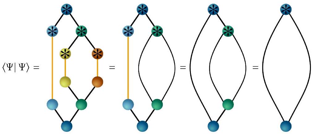
      لاحظ أننا نفسر ML-MCTDH و DMRG كخوارزميات معينة لحل معادلة شرودنغر باستخدام نفس فرضية TTNS. مع هذه التفسير، يمكن استخدام DMRG لـ MPSs و TTNSs على الرغم من أنه تم تقديمه كطريقة لتقريب الحالات الأساسية كـ MPSs.
      تم تقديم بعض الترجمات غير المكتملة بالفعل، على سبيل المثال، في المراجع [23، 59، 73-76].
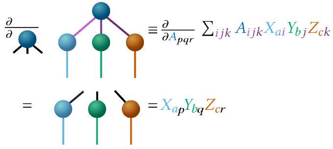
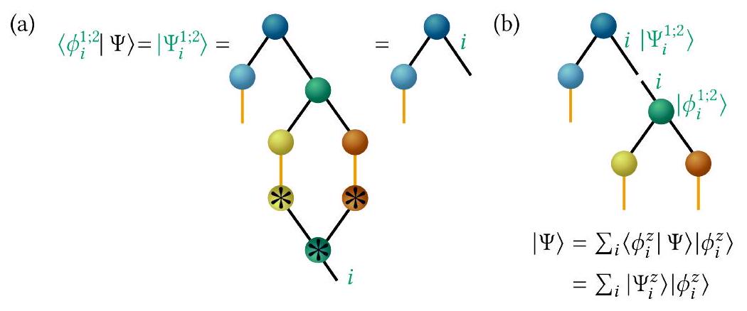
  1. لتجنب تعريف “حالات الجسيم الفردي”، سنستخدم هنا مصطلح “دالة” لكلا الحالتين وتمثيلها، على سبيل المثال، في فضاء الموضع، تبدأ العديد من اشتقاقات MCTDH عادةً بتعريف SPFs كدوال فعلية ثم تستخدم تدوين ديراك لعناصر المصفوفات والمشروعات. هنا، نفضل استخدام تدوين ديراك طوال الوقت.
    لاحظ أن الطريقة المسماة MCTDHF من قبل ييجر ويورغنسن هي في الواقع نهج CASSCF استجابة وبالتالي ليست تعتمد على الزمن بشكل صريح. ومع ذلك، فقد استخدمت المنشورات ذات الصلة بالفعل مبدأ التباين المعتمد على الزمن.
  2. لاحظ أنه في المرجع [59] نستخدم ترميزًا مختلفًا حيث يعني الموضع الأفقي في الطبقة . ثم إعطاء و يكفي تحديد موقع SPF في الشجرة.
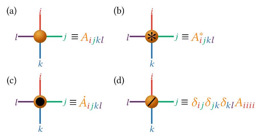
    لاحظ أن فندريل وماير يستخدمان نفس الرمز ولكن بتعريف مختلف [96]، حيث لا يحتوي على الذي يضاف إلى الرموز بشكل منفصل.
  3. هناك العديد من الروابط الافتراضية الممكنة ولكنها نادرة. انظر أدناه في المعادلة (12) لمثال مقدم من SHF ذو الفهرسة المزدوجة.
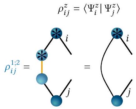
    يمكن أيضًا تفسير الرابطة الفيزيائية على أنها الفضاء الفرعي المتجه الذي ينتمي إليه الحالة. ثم يمثل مخطط TTNS في الواقع حالة. وليس تمثيلاً معيناً.
    في حالات خاصة مثل SHFs الطبيعية، يمكن أن تكون الروابط الافتراضية الموجهة لأسفل متعامدة ولكن ليست متعامدة طبيعية، انظر القسم الخامس.
  4. يرجى ملاحظة أننا نتعامل مع مستقل عن .
  5. ك remark فني، يجب توخي الحذر بالنسبة للموترات الموضوعة عند فروع الشجرة لتعميمها مرة واحدة فقط. يجب تخطي هذه الموترات خلال أجزاء من المسح بحيث يتم تعميمها مرة واحدة فقط في كل مسح. انظر المراجع [116، 151-153] لمزيد من التفاصيل.
  6. يمكن تجنب الانعكاس الصريح وحل نظام خطي بدلاً من ذلك. هذا أكثر استقرارًا من الناحية العددية ولكنه لا يخفف من مشكلة التفرد، مع ذلك.
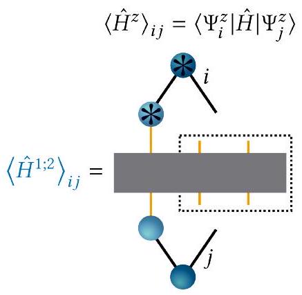
    تحويل الموتر إلى مصفوفة وإسقاط الـ ملصق، . ثم تحتوي معادلات حركة SPF على , وهو المعكوس الزائف لمور-بينروز والذي يمكن تنظيمه مباشرة، على سبيل المثال، من خلال SVD.
  7. توسيع هذا ليشمل SHFs غير الطبيعية أمر سهل.
  8. هذا يطبق جهاز SHF مرتين. حيث أن الأجهزة ذاتية التكرار، فإن هذا يعادل تطبيق الجهاز مرة واحدة فقط، كما هو موضح في المعادلة (50).
    لا تزيد أجهزة SHF وSPF من تكلفة الحسابات في المعادلة (56).
    تم مناقشة هذا أيضًا في المرجع [191].
  9. لاحظ أنه في التنفيذ الفعلي، بسبب عدم التغير في القياس، فإن تبادل SPFs وSHFs يؤدي إلى قيم عددية مختلفة، اعتمادًا على كيفية جعل SHFs متعامدة.
  10. يمكن تشكيلها إما باستخدام أجهزة SHF وSPF أو صراحة عن طريق إنشاء مساحة فارغة [194].
    لاحظ أن هذه التقريبات المعتمدة على SVD [193،197] تستخدم مصفوفات مؤقتة تتناسب مع أبعاد الربط وعدد حدود المجموع في هاملتونيان SoP (أو، بشكل مكافئ، أبعاد الربط MPO). حيث يمكن أن يكون هناك أكثر من حدود في التطبيقات النموذجية، مما قد يؤدي إلى مصفوفات كبيرة بشكل غير معقول ويجب إدخال تقريبات إضافية، على سبيل المثال، من خلال النظر فقط في أجزاء من الهاملتونيان الكلي لتغني الفضاء الفرعي.
    مع دمج الوضع، يمكن أن يكون حجم الأساس الفيزيائي الفعال أكبر بكثير من ; انظر الشكل 34 لمثال.

Journal: Molecular Physics, Volume: 122, Issue: 14
DOI: https://doi.org/10.1080/00268976.2024.2306881
Publication Date: 2024-02-12

A tensor network view of multilayer multiconfiguration time-dependent Hartree methods

Henrik R. LarssonDepartment of Chemistry and Biochemistry, University of California, Merced, CA 95343, USA*

Abstract

The multilayer multiconfiguration time-dependent Hartree (ML-MCTDH) method and the density matrix renormalization group (DMRG) are powerful workhorses applied mostly in different scientific fields. Although both methods are based on tensor network states, very different mathematical languages are used for describing them. This severely limits knowledge transfer and sometimes leads to re-inventions of ideas well known in the other field. Here, we review ML-MCTDH and DMRG theory using both MCTDH expressions and tensor network diagrams. We derive the ML-MCTDH equations of motions using diagrams and compare them with timedependent and time-independent DMRG algorithms. We further review two selected recent advancements. The first advancement is related to optimizing unoccupied single-particle functions in MCTDH, which corresponds to subspace enrichment in the DMRG. The second advancement is related to finding optimal tree structures and on highlighting similarities and differences of tensor networks used in MCTDH and DMRG theories. We hope that this contribution will foster more fruitful cross-fertilization of ideas between ML-MCTDH and DMRG.

I. INTRODUCTION

The multiconfiguration time-dependent Hartree (MCTDH) method and the density matrix renormalization group (DMRG) were developed nearly simultaneously in the fields of molecular quantum dynamics and condensed matter physics, respectively . Both methods have greatly influenced their respective field and continue to do so. This may be seen most clearly by noticing that MCTDH and DMRG are being used outside their initial field of research and are now established in other fields such as initio molecular electronic structure [5-8] in the case of DMRG and strong-field electron dynamics in the case of MCTDH [9-15], among many other examples. Initially, MCTDH and DMRG focused on very different areas and applications. MCTDH is based on the time-dependent Schrödinger equation (TDSE) whereas the DMRG is based on the time-independent Schrödinger equation (TISE). Around 20 years after their foundations, both methods were extended. The less flexible MCTDH wave function ansatz (relative to the DMRG), a Tucker decomposition [16], was improved by the development of the multilayer MCTDH method (ML-MCTDH) [17-19], where a tree tensor network state (TTNS) or hierarchical Tucker format [20-26] is used. For the DMRG, the focus on the TISE was broadened by extensions to real-time evolution [27-30]. Furthermore, the wavefunction ansatz of the DMRG, a matrix product state (MPS) [31-35], which is a subset of TTNSs, was later extended to TTNSs [36-40]. Inspired by the DMRG, other methods that extend TTNSs to general tensor network states (TNSs) have been developed [41-50]. These different individual developments led to very different mathematical “languages” used to describe DMRG, ML-MCTDH, MPSs and TTNSs. In fact, describing DMRG using MPSs even is a more recent concept that differs dramatically from the original DMRG language [35, 51]. This language barrier is becoming more severe as more and more DMRG approaches are used in systems typically treated with (ML-)MCTDH and vice versa [52-72]. It is very difficult to analyze similarities and differences of methods developed by these two communities, even when these methods actually are very similar or virtually identical.
Here, with a focus on ML-MCTDH, we will highlight connections between ML-MCTDH and DMRG by “translating” MCTDH expressions into the diagrammatic language that is extensively used in TNS community but so far has not come to full use in the ML-MCTDH community. We hope that these translations will show more clearly the connections between ML-MCTDH, DMRG and TNSs. We will highlight the power of the diagrammatic language by deriving the ML-MCTDH equations of motions through diagrams. We will discuss an alternative way to solve the ML-MCTDH equations of motions, which is given by time-dependent and time-independent DMRG approaches. Furthermore, we will show connections between DMRG and ML-MCTDH advancements exemplified by two advanced topics, (1) subspace enrichment (optimal unoccupied single particle functions, SPFs), and (2) optimal TTNS structures, which also includes a discussion of why MPSs are preferred in molecular electronic structure, compared to TTNSs in vibrational quantum dynamics.
Our outline is as follows: Sections II and III briefly review the ML-MCTDH and tensor network languages, respectively. Sections IV and V “translate” standard (ML-)MCTDH expressions and the ML-MCTDH equations of motions, respectively. Section VI fully derives the ML-MCTDH equations of motions solely using diagrams. Section VII reviews TTNS canonicalization/orthogonalization procedures and DMRG-typical sweeps. A time-dependent DMRG approach that can be viewed as counterpart to the ML-MCTDH equations is reviewed in Section VIII and used for describing the time-independent DMRG
in Section IX. Sections X and XI deal with two advanced topics on unoccupied SPFs and on tree structure optimizations. We conclude in Section XII.

II. THE MULTILAYER MULTICONFIGURATION TIME-DEPENDENT HARTREE ANSATZ

To solve Schrödinger’s equation, the standard full configuration interaction (FCI) approach is a Ritz-Galerkin ansatz [26,77], where the -dimensional wavefunction is represented by a direct product of “primitive” bases of finite size in each dimension :
Here, we use Dirac’s notation [78, 79] and assume an orthonormal primitive basis. Further, we will only discuss the case of distinguishable particles (or an appropriate mapping of indistinguishable particles, such as the Jordan-Wigner transform) and thus do not assume any (anti-)symmetry in the real- or complex-valued coefficient tensor , whose entries are then to be determined.
In most molecular quantum dynamics applications, the primitive basis is a spectral or pseudospectral grid-like basis given by the discrete variable representation (DVR) [80-85], which, among others, is also known as Lagrange-mesh method [86] in some Physics literature and as cardinal basis in some applied mathematics literature [84, 87]. Note that nonlinear bases, in particular Gaussians, are possible as well [88, 89].
The FCI ansatz in Eq. (1) is exact in the space of the primitive basis (given no further approximations on the Hamiltonian) but the number of entries in the coefficient tensor scales as , where is the geometric mean of the basis sizes . To avoid this prohibitive scaling, the (ML-)MCTDH ansatz approximates Eq. (1) by expanding in another orthonormal basis, the so-called single-particle functions (SPFs) The difference between the primitive basis and the SPF basis is that the latter is variationally optimized and thus fewer basis functions are required. The (ML-)MCTDH ansatz then takes the form of
Note that the SPFs may be multidimensional (thus ); see below. The superscript 1 in and in denotes the layer in ML-MCTDH. For time evolution, both the -dimensional tensor and the SPFs are optimized according to the Dirac-Frenkel-McLachlan time-dependent variational principle (TDVP) [90-94].
Some remarks on the notation that is used here: For consistency with the main body of ML-MCTDH literature, here we closely but not exclusively follow the notation of Manthe [19, 95]. It only marginally differs from that of Meyer and Vendrell [96], but there are some differences to the notation used by Wang and Thoss (e.g., the counting of layers differs) [18, 97]. Notably, all of these notations are based on the original MCTDH formulations [1,2]. A different notation exists in the mathematics community [98-102]. A non-exhaustive comparison of used symbols in the MCTDH, mathematics, and tensor network communities is given in Table I.
The ansatz in Eq. (2) is very flexible and there are three main realizations of it: (1) In the simplest MCTDH ansatz, the SPFs are one-dimensional and . The SPFs are then represented by the same time-independent, primitive basis used in the FCI ansatz, Eq. (1). MCTDH then has the same exponential scaling as the FCI ansatz, but the base is reduced as the SPFs are optimized and thus fewer of them are needed, compared to the primitive basis.
(2) For MCTDH with mode combination [103], and the SPFs are expressed in terms of a multidimensional ( dimensional) basis. Typically, this basis is a direct-product basis, but it also can be a non-direct-product basis [104-106]. The multidimensional degrees of freedom that describe the multidimensional SPFs are then denoted as “logical.” Mode combination is useful for describing strongly correlated degrees of freedom. For systems with , mode combination often leads to a better efficiency than the normal MCTDH ansatz. In the context of molecular electronic structure, an antisymmetrized MCTDH ansatz with mode combination is equivalent to the time-dependent complete active space self-consistent field (TD-CASSCF) algorithm [107-111]. This is also called multiconfiguration time-dependent Hartree-Fock, MCTDHF [9-15]. In TD-CASSCF,
TABLE I. Some notation used in this work and in MCTDH literature. A non-exhaustive list of alternative symbols used in MCTDH, mathematics, and DMRG literature is given, also. See Fig. 1 for a concrete example of the usage of some of the symbols.
description symbol alternative symbols
physical dimension
physical (“primitive”) basis state
physical basis dimension
number of layers L
layer
SPF basis state
horizontal position in layer
node/SPF position
layer and node/SPF position
coefficient tensor position
node/tensor/site/SPF dimension
bond dim./rank/SPF basis size
generic SPF basis size
total size of basis representing SPF
SPF index
SPF composite index
SHF composite index
SPF tensor/site
configuration
single-hole function (SHF)
SHF configuration
SPF projector
SHF projector
single-particle density matrix
mean-field operator
gauge operator
one-dimensional Hamiltonian term
the three-dimensional SPFs describing one electron would be called molecular orbitals and the primitive basis functions would be called atomic orbitals.
(3) For ML-MCTDH, holds as well, but the -dimensional SPFs in Eq. (2) are expanded recursively using the very same MCTDH ansatz, i. e.,
are then either described by the primitive basis (possibly with mode combination) or they are again expanded using the MCTDH ansatz. This is repeated recursively until the last layer is reached.
The recursive structure of the ML-MCTDH ansatz can be represented using tree diagrams [19] as shown in Fig. 1, which also gives an example of some ML-MCTDH notation. In the ML-MCTDH context, these diagrams are almost exclusively used to depict the tree structure of a particular ML-MCTDH wavefunction. Only recently have they been used to represent some other MCTDH-related quantities [59, 75, 76, 116]. As we will show below in Section III, there is a direct connection of these ML-MCTDH diagrams to the tensor network diagrams used in DMRG literature [30, 35, 48, 59]. Among others, we will further show how these diagrams can be used for deriving the ML-MCTDH equations of motions.
In the commonly used notation, the -dimensional SPFs of layer are denoted by . The additional symbols, specify the exact location of the SPFs in the tree. The indices are determined by traversing the tree using depth-first search starting at . During the traversal, the horizontal position of the path through the tree taken at layer is given by .
To avoid dealing with the cluttered notation used for indexing and specifying the locations of tensors and functions in the
FIG. 1. Example ML-MCTDH tree/TTNS displaying the notation. Bonds (vertices) denoting physical indices corresponding to primitive basis functions are shown in orange. Their size is given by but also implicitly through . Bonds denoting “virtual” indices for single-particle functions (SPFs) are shown in black. The tree has layers. Their basis sizes are , their dimension is , and the total number of SPFs at one node is . Note that the SPF is described by the tensor and those from lower nodes connecting to . Some of the SPFs and SPF coefficient tensors are shown as well. The tensors that describe two particular SPFs are marked by dotted rectangles.
tree, MCTDH developers often simplify the notation by defining the composite index , which specifies the entries of the tensors . Depending on the context, can also specify a raveled index with range with
We further simplify the notation by defining the compound indices , and specifies the layer and location of an SPF, and that of an SPF tensor. This simplified notation leads to a more compact description of the SPFs as
where
are the configurations.
Armed with this simplified notation, we introduce the counterpart of the SPFs, the single-hole functions , which are defined by projecting the corresponding SPFs onto the ML-MCTDH state , i.e.,
Using the orthonormality conditions of the SPFs, we can describe as sum of product of SHFs and SPFs,
The SHFs are useful for defining effective operators, as shown below in Section V A.
In traditional DMRG language [4, 35, 51], Eq. (8), corresponds to using single-site DMRG and expanding the state in terms of a system block, , and an environment block, :
where the system block is given in MCTDH notation by the SHFs and the environment block is given by the SPFs.
FIG. 2. Example of mapping a tensor to a node with four vertices/bonds in a tensor network diagram. Panels (b)-(d) show additional notations introduced here for specifying complex conjugation (b), time-derivative (c), and diagonal tensors (d).
FIG. 3. Two exemplary tensor contractions. Shown are the individual tensors, the actual tensor network diagrams, where bonds/vertices corresponding to the indices that are contracted over are connected, as well as the mathematical equations. (a) shows the contraction of an MCTDH state/Tucker tensor decomposition. (b) shows the ths entry of the product of the matrices , and .

III. TENSOR NETWORK DIAGRAMS

The complete tensor contraction pattern to retrieve the full ML-MCTDH state/TTNS represented by the primitive basis from the tensors/SPF representations actually is given by the diagram shown in Fig. 1. This is possible by introducing a means of translating these types of tensor network diagrams to mathematical equations. Since the 19th century, scholars have described tensor algebra using graphical notations [117-119]; see Ref. [120] for an overview. Tensor network diagrams were first used by Penrose in the 1950s [121] and can be highly useful not only to visualize but also to derive mathematical expressions [30, 35, 47, 48, 122, 123]. The notion of tensor networks leads to TNSs. In a tensor network diagram, each tensor is represented as a node and each of the tensor’s indices are represented as edges or “bonds;” see Fig. 2 for a representative example. Some additional definitions are often introduced. In the following, an asterisk on top of the node denotes complex conjugation. A dot denotes the time-derivative of a tensor and a diagonal line denotes diagonal tensors, as shown in Fig. 2. As the TTNS is the wavefunction ansatz of the ML-MCTDH method, in the following, the terms TTNS and ML-MCTDH state are used interchangeably.
Similar to Einstein’s summation convention [124], contractions of tensors (summations over common indices) are defined by connecting the common bonds (edges) of those nodes whose corresponding indices should be contracted. Fig. 3 depicts two examples.
Tensor network diagrams are not only helpful to visualize tensor contractions, but they also can be used to derive equations and to denote specific properties. Fig. 4 shows an example of calculating the derivative of a tensor network through a diagram.

IV. TENSOR NETWORK DIAGRAMS IN COMPARISON TO MCTDH LANGUAGE

Aiming at comparing the MCTDH language with tensor diagrams, here we give a translation of commonly used MCTDH expressions. We will use the ML-MCTDH state/TTNS shown in Fig. 5 as example. Note that, given the flexibility of TTNSs in terms of their structure, TTNS equations are best represented with the help of example trees. Generalizations to other tree structures are straightforward. This is different to MPSs or projected entangled pair states, since those TNSs have simpler structures (one- or two-dimensional grids, respectively).
FIG. 4. Example of how to use diagrams to derive mathematical expressions. Shown is the derivative of the tensor network from Fig. 3 (a) with respect to , i.e., .
FIG. 5. Example ML tree/TTNS that is used here for deriving ML-MCTDH expressions. The TTNS has three layers and describes a threedimensional state.
In the diagram of a TTNS, indices that are free “dangling” bonds, i. e., that are not connected to another node, are called physical. In tensor network diagrams, all other bonds of a TTNS are called virtual. Physical and virtual bonds cannot always directly be distinguished in more general diagrammatic expressions and need to be inferred from the initial TTNS. To simplify this, in the following diagrams, we will always color physical bonds orange and virtual bonds black. Here, each tensor has its own specific color, as given in Fig. 5. In tensor network diagrams, the number of SPFs, , corresponds to the dimension of a bond and hence is also called bond dimension (sometimes also rank in mathematics or number of kept states, , in traditional DMRG language; compare with Table I). In the following we will use when referring to the bond dimension/number of SPFs in general and when referring to a specific node. The dimensions of the physical bonds are given as that of the primitive basis.
Unlike a complete TTNS, functions such as SPFs or SHFs do have free virtual bonds. Any function must contain one or more free physical bonds and, typically, one single free virtual bond that denotes the function number (e.g., in ). The physical bonds then denote the function values. Orthonormality is often depicted either by using arrows instead of bonds or by using special symbols for the nodes such as triangles. Here, we follow the convention from ML-MCTDH and some mathematics literature [23,26,98] and depict orthonormality by the direction of the virtual bonds. If the virtual bond is pointing upward (toward layer 1, away from the physical bonds), then the function/tensor is orthonormal. Note that there always is only one single virtual bond pointing upward. If the virtual bond is pointing downward (toward the physical bonds/the last layer), then the function/tensor is nonorthonormal.
An example of a configuration (group of SPFs/nodes) is shown in Fig. 6 together with a contraction of the configurations with a coefficient tensor, which leads to an SPF. Examples of SPFs in comparison to single coefficient tensors are shown in Fig. 7. A coefficient tensor is just a single node and its connecting bonds. The values of can be obtained from the SPFs
FIG. 6. Example configuration. Shown are from Fig. 5 in the dashed rectangle. A contraction of with , leads to the SPF .
FIG. 7. Diagrams of SPFs in comparison to tensors. Four examples of SPFs and tensors taken from Fig. 5 are shown. (a) and (c) are SPFs as they contain physical bonds. (b) and (d) are tensors as the diagrams only contain a single node. The node in (c) is identical to that in (d) and can be interpreted either as SPF or tensor, depending on the context.
FIG. 8. Example of matricization and orthonormal matrices as diagrams. (a) Matricization of the tensor into , where is a composite index for and . (b) Diagrammatic notation of the orthonormality of and, equivalently, . The straight line denotes a unit matrix.
by projecting all SPFs connecting to onto , compare with Eq. (5) and (6). Note that for the last layer in the tree, a node can be interpreted either as tensor or as SPF, see Fig. 7(c) and (d). Which interpretation is used depends on the context. is called root tensor and the corresponding node is called root node.
It is often useful to reshape (and permute) a tensor into a matrix, which is called matricization (or flattening or matrix unfolding) [23]. For example, a tensor of size may be permuted and reshaped into a matrix by using the mapping where is a composite index . This is helpful for realizing orthonormality relationships, e. g., , or more explicitly, and, equivalently, . Fig. 8 gives an example of matricization and orthonormality relationships in diagrams.
In ML-MCTDH, the orthonormality of the SPFs means that each of the tensors used to construct the SPFs in a diagram can be matricized into orthonormal matrices of size , where is the total size of all the bonds pointing downward, as defined in Eq. (4). In this case, the matricization is performed by using the composite index (corresponding to the bonds pointing downward, toward the physical bonds) in as row index and the SPF index (the bond pointing upward to the root node) as column index; thus . This leads to extremely useful simplifications of the diagrams. For example, the squared norm of an ML-MCTDH state, , simply is given by that of the root node coefficient tensor, . This is shown diagrammatically in Fig. 9.
The computation of the overlap, , and the projector onto an SPF space,
are shown in Fig. 10. Due to the orthonormality, reduces to . Note that even though formally the SPFs are orthonormal, in practice the finite accuracy of the ML-MCTDH differential equation solver leads to small nonorthonormality errors of the SPFs. In MCTDH implementations, this error is neglected in the tensor contractions, but the SPF projector is modified to take
FIG. 9. Diagram of the overlap of a TTNS with itself (squared norm). The TTNS from Fig. 5 is used as example. The orthonormality relationships of the SPFs greatly simplify the diagram. Compare with Fig. 8 (b).
FIG. 10. SPF overlap (a) and projection (b). from Fig. 5 is used as example. For the overlap of orthonormal SPFs, compare with Fig. 8 (b).
the spurious nonorthonormalities into account via [125]
where is the overlap matrix of .
An example of an SHF is shown in Fig. 11. In contrast to the SPF, for an SHF the function index corresponds to a downward (and not upward) pointing virtual bond and thus an SHF is nonorthonormal. They can be made orthogonal, however; see Section V A. The relationship between the SHF-SPF decomposition in ML-MCTDH and the system-environment decomposition in traditional DMRG, Eq. (9), is shown in Fig. 12 (in this case we make an exception and show an MPS instead of the TTNS from Fig. 5).
The SHF definition can be generalized to doubly-indexed SHFs defined as [19]
where we have highlighted the two “hole indices” and by colors. An example is shown in Fig. 13. Doubly-indexed SHFs
FIG. 11. Example of a single-hole function (SHF), its construction and usage. (a) Construction of SHF from Fig. 5 through projection of onto . Orthonormality relations simplify the SHF, compare with Fig. 8 (b). (b) Simplified together with its counterpart, the SPF . Contracted over , they form the total TTNS .
FIG. 12. Comparison of ML-MCTDH diagram and traditional DMRG language. (a) The decomposition of an ML-MCTDH state/MPS in terms of a single-hole function (SHF) and a single-particle function (SPF); compare with Fig. 11. (b) Single-site DMRG setting with a system and an environment block. The system (environment) block is spanned by the SHF (SPF) space; compare with Eq. (9).
allow for a recursive definition of the SHFs:
In a diagram, the doubly-indexed SHF simply is represented by two virtual bonds, one pointing downward and one pointing upward; see Fig. 13 (b).

V. ML-MCTDH EQUATIONS AND CONNECTION TO DIAGRAMS

The ML-MCTDH equations are based on the ML-MCTDH ansatz, Eq. (2), and the TDVP,
FIG. 13. Example of a doubly-indexed single-hole function (SHF) and its usage. (a) from Fig. 5 as example of a doubly-indexed SHF. (b) (see Fig. 11) together with . Contracted over , they form the SHF .
FIG. 14. Diagram of a single-particle density matrix for the TTNS from Fig. 5. Compare with Eq. (17).
where denotes first-order variations of with respect to its parameters. In the following, we will set . For the ML-MCTDH wavefunction ansatz, Eq. (14) is solved subject to two constraints: Firstly, the orthonormality conditions of the SPFs, and secondly, their gauge invariance,
where is some arbitrary, hermitian constraint operator and denotes the time derivative of . The gauge invariance is discussed more in Section VII. In short, unitary transformations of the SPFs/SHFs alter neither orthonormality nor the state. This leads to an arbitrariness of the SPFs that is manifested by the gauge invariance. This arbitrariness is fixed by Eq. (15). Various choices of exist and here, for simplicity, we will use one of the most common choices and simply set it to zero [1], i.e.,
Generalizing the following equations to non-zero is straightforward and some aspects of using a different gauge will be discussed in Section VIII.

A. Density matrices and mean fields

Before we proceed with defining the equations of motions, we will define two additional quantities and provide diagrammatic expressions for them. The “single-particle” density matrix is defined as
and it is equal to the transpose of the one-particle reduced-density matrix in electronic structure theory [111]. In addition, it is related to the Gram matrix with entries of with parameters , which is used in similar theories [23,54,55,57,127,128]. SPF orthonormality simplifies the computation of and an example is shown in Fig. 14. Diagonalizing it yields natural SPFs and SHFs. The eigenvalues of are called natural occupations. The SHFs with nonvanishing natural occupations are then orthogonal, but not orthonormal.
The mean-field operators are defined as
where we have inserted the definitions for the SHFs in the second equation to highlight that Eq. (18) still defines an operator and not a scalar. Hence, is a matrix of operators. An example diagram that highlights the “operator part” and the “matrix part” (indices and ) of Eq. (18) is depicted in Fig. 15.

B. Equations of motions

Using the definitions of the mean-field matrices and density matrices, we now give concise expressions of the ML-MCTDH equations of motions. Eq. (14) together with Eq. (16) leads to the following equations of motions for the SPFs [2]:
FIG. 15. Diagram of a mean-field matrix for the TTNS from Fig. 5. The dashed rectangle corresponds to the “operator part” of the mean-field matrix and the indices specify the “matrix part.” Compare with Eq. (18).
Note that in practice the single-particle density matrix can be singular and typically needs to be regularized [2], but alternatives exist ; see also Section X. We will make Eq. (19) more explicit by projecting the corresponding configurations onto Eq. (19) so that the equations of motions for the SPF coefficient tensor are obtained as
For the root tensor in the first layer we obtain standard Ritz-Galerkin-like [26,77] equations of motions for the TDSE expressed in a finite (but time-dependent) basis:

C. Some common forms of the Hamiltonian

The most common form of and other operators used by MCTDH and many other methods is a sum-of-product form (SoP), where the Hamiltonian is decomposed as a sum of direct products of one-dimensional operators:
In the second part of Eq. (22) we have absorbed the complex-valued coefficients into one of the operators , for clarity. This Hamiltonian has the advantage that its application on a state has a relatively simple but favorably-scaling implementation [131, 132] based on one single loop over well-optimized matrix-matrix multiplications [133].
The counterpart to the SoP Hamiltonian in the DMRG community is the matrix product operator (MPO) [26,35,134,135], which is defined as
An MPO is a generalization of an MPS to an operator. Likewise, a tree tensor network operator can be defined as generalization of a TTNS to an operator [26]. In the MCTDH community, for diagonal potential operators this is known as multilayer potfit format [136], whose advantages and disadvantages so far have not been fully explored [137], however.
The SoP Hamiltonian can be represented as a MPO that is diagonal in bond dimension [138, 139]: Defining as raveled compound index , Eq. (22) can be mapped onto Eq. (23) by the relation
The SoP Hamiltonian and its mapping to an MPO is shown diagrammatically in Fig. 16.
FIG. 16. Diagram of a sum-of-product (SoP) operator and mapping to a particular matrix-product operator (MPO) with diagonal tensors. Here, the dotted, diagonal line in the MPO tensors indicate tensors diagonal only with respect to the virtual bond dimension (black lines). The orange lines denote the physical space. Compare with Eqns. (22)-(24).
FIG. 17. Diagram of a matrix representation of a mean-field sum-of-product operator for the TTNS from Fig. 5. The partitioning of this diagram into one single-hole function term (mean field “matrix part”) and one configuration term (mean field “operator part”) is visualized by dotted rectangles. Compare with Eq. (26) and Fig. 15.
For the ML-MCTDH equations, Eq. (20), it is useful to rewrite in terms of an operator that acts solely on the same space as that spanned by the configurations , and in terms of an operator that acts on the remaining space [19, 96]:
is defined recursively in the same way as the SPFs, making this partitioning similar to the SHF-SPF expansion of a TTNS, Eq. (8). A virtually identical partitioning exists for the DMRG and this partitioning is trivially fulfilled both for SoPs and MPOs. Then the “matrix” representation of the mean-field operator, Eq. (18), which is a given by a four-dimensional tensor, can be represented as
An example diagram is shown in Fig. 17. Note that both the mean-field operators and the density matrices can be evaluated efficiently in a recursive way starting at the first layer for the density part and starting at the last layer for the operator part [19]. This is related to the site-per-site contraction of overlaps in the DMRG [35, 48].

VI. DERIVATION OF ML-MCTDH USING DIAGRAMS

Here we will use tensor network diagrams to derive the ML-MCTDH equations of motion (20) and (21). For solving the TDVP, we need the first-order variations . They are related to the derivatives of the TTNS with respect to all of its individual tensors components, which we specify here as :
FIG. 18. Derivatives of a TTNS. First-order variation of , which contain derivatives with respect to the individual tensors (upper panel), and time derivative (lower panel) for the TTNS from Fig. 5. Tensors denoting variations are marked with a .
Inserting into the TDVP, Eq. (14), leads to as many terms as there are parameters in the TTNS for , and we get
Since the variations are arbitrary and independent of each other, each of the terms in Eq. (28) must vanish independently of each other and independently of the variations [91]. Hence, we get the following set of equations
Here, it will be useful to use the tensor structure to rewrite Eq. (30) in terms of the individual tensors of the TTNS,
Together with the gauge conditions Eq. (16), each of these equations will lead to the equations of motions for a particular tensor.
For the derivations of the equations of motions for each tensor, we again use the TTNS from Fig. 5 as a simple example but note that this can be easily generalized to any TTNS, including TTNSs with more layers. The first-order variation and time-derivative of are shown in Fig. 18.
We start the derivation with the first term of in Fig. 18, which is for the root node, . Inserting this into Eq. (31) leads to the expression in Fig. 19(a). Because we demand that the projection of an SPF onto its time-derivative is zero, Eq. (16), most of the terms arising from vanish, and, using the SPF orthogonality relationships, Fig. 10, straightforwardly we obtain Eq. (21), which is shown diagrammatically in Fig. 19(b).
Next we turn to the equations for from the TTNS in Fig. 5. The derivation is shown in Fig. 20. Inserting the just-derived Eq. (21), we obtain a specific form of Eq. (20) for this node. Compared to the more general Eq. (20), there are two variations: Firstly, since a next layer does not exist for , here the configurations from Eq. (21) just correspond to the primitive basis representation. Secondly, in Fig. 20 we moved to the left-hand-side in Eq. (20), which is closer to the original MCTDH derivation and hints at other ways to solve for this equation, namely by using the pseudo-inverse of [1,130] (see
FIG. 19. Derivations of the equations of motions for the root tensor (shown in the upper left rectangle) for the TTNS from Fig. 5. The Hamiltonian is denoted by the gray rectangle. The individual terms come from Fig. 18. After making use of the SPF orthogonality relationships, Fig. 10, and the SPF gauge, Eq. (16), one arrives at panel (b), which corresponds to Eq. (21). The dotted rectangle in the lower right of panel (b) highlights .
also Refs. [127, 140] and Section XA). Note that the just-derived equations for and are sufficient to fully program the plain MCTDH equations of motions without the multilayer form.
The derivations for the equations for is very similar to that of and shown in Fig. 21. The main difference is that here we actually have configurations appearing in the diagrams. This is because is not connected to any primitive basis, which only happens in ML-MCTDH and not in plain MCTDH for non-root-tensors.
We now turn to the derivations for the tensors in the third layer. Since is not any different from , we will focus on only one of them. Inserting into Eq. (31) leads to the diagrams shown in Fig. 22. Compared to the derivation for the first and second layer, here the derivation is slightly more involved as we have to take the equations of the previous two layers into account. We first simplify two terms appearing on the left-hand side of Fig. 22(b). For that we combine the results from Fig. 19 and Fig. 21, which gives the expression shown in Fig. 23. Note that two terms on the right-hand site of Fig. 23 cancel each other. Inserting this back into Fig. 22(b) leads to the final equations of motions as shown in Fig. 24. This corresponds to Eq. (20) for layer 3.
We note that next to the “standard” approach that we use here [ ], an alternative approach to derive the ML-MCTDH equations of motions exist . There, one first derives the projector that projects onto the tangent space, that is, the space spanned by the first-order variations. Then one solves
can be written as , where is the inverse of the Gram matrix. With this formulation of one obtains the standard ML-MCTDH equations of motions [142-144]. Using a different expression of , this approach will become important for the TDVP-DMRG scheme discussed in Section VIII.

VII. CANONICALIZATION: CHANGE OF ROOT NODE AND SWEEPS

Here, we will discuss how to change the root node of the ML-MCTDH state/TTNS without changing the actual state that is represented, which is at the heart of DMRG algorithms. This “canonicalization” exploits that the TTNS is invariant under
FIG. 20. Derivations of the equations of motions for (shown in the upper left rectangle) from the TTNS shown in Fig. 5. Terms that are trivially zero due to the gauge conditions have been set to zero immediately (compare with Fig. 19). The SPF orthogonality relationships, Fig. 10, and the expression from Fig. 19 have been used in panel (b) to simplify the expression in (a). This is marked by gray ellipses.
FIG. 21. Same as Fig. 20 but for .
FIG. 22. First part of the derivation of the equations of motions for (shown in the upper left rectangle) from the TTNS shown in Fig. 5. Terms that are trivially zero due to the gauge conditions have been set to zero immediately (compare with Fig. 19). SPF orthonormality simplifies the expression in (a), as shown in (b) (compare with Fig. 9).
transformation by an invertible matrix . This is seen by inserting into the SHF expansion, Eq. (8):
where we introduced the -transformed SHFs and SPFs ,
This is depicted diagrammatically in Fig. 25(a).
T can be chosen to orthogonalize and normalize the SHFs. This then leads to nonorthogonal T-transformed SPFs. Since SPFs should be orthonormal, however, now we can re-interpret Eq. (34) and just exchange the meanings of the T-transformed SHFs and SPFs by formally turning the now orthonormal SHFs into SPFs and vice versa. This leads to a change of the tree structure. Additionally, if the transformation is done for the first layer, the root node changes. This is shown in Fig. 25(b).
In practice, due to orthonormality of all SPFs in the TTNS, to orthogonalize and normalize the SHFs one only needs to orthogonalize the tensor with entries . This is done by first transposing it to with entries , where and correspond to the labels for the tree structure with changed root node. Then is matricized (compare with Fig. 8) and orthogonalized. The matrix orthogonalization and normalization can be done, e. g., using a QR matrix decomposition, which corresponds to Gram-Schmidt orthogonalization [23, 145]. The in the QR matrix then corresponds to in Eq. (36) and is absorbed in the tensor connecting to . This procedure, also sometimes dubbed isometrization [39], together with the different orthonormality conditions (isometries) of the initial root tensor is shown diagrammatically in Fig. 26.
Note that this change of canonicalization can be done with any SPF-SHF pair in the tree and not only that of layer 1. Further, the canonicalization allows us to systematically traverse the tree in a way that every tensor at some point will become at least
FIG. 23. Expression for two diagrams on the left-hand site of Fig. 22(b). The gray-lined (gray-dashed) ellipses show the expression from Fig. 19 (Fig. 21). Note that the first and last term on the right-hand site cancel each other.
FIG. 24. Final expression of the equations of motions for (shown in the upper left rectangle) from the TTNS shown in Fig. 5. To arrive at this, the expression from Fig. 23 is inserted in Fig. 22.
once a root node. This is an important ingredient in any DMRG algorithm and called sweep. It can be implemented using graph algorithms such as depth-first search; see Fig. 27 for an example. Other ways to traverse a TTNS in one sweep are possible as well [39].
As technical remark, instead of using a QR decomposition to orthogonalize the SHFs one can also use other orthogonalization procedures such as singular-value-decomposition (SVD) [23,145] (using in the SVD as orthogonal matrix and SV as ). This is equivalent to using the eigenvectors of the reduced density matrix. Hence, this leads to natural SPFs, which often result in improved numerics as then the Hamiltonian represented by the basis of the configurations often is diagonally dominant. SPFs that diagonalize the separable part of the Hamiltonian are another commonly used choice to improve numerics [146]. All of these choices realize a particular gauge.

VIII. TIME-DEPENDENT DMRG APPROXIMATION

One major problem of the ML-MCTDH equations of motions is that they can become highly nonlinear. Hence, sophisticated integrators need to be used for efficient propagation [94]. To overcome this for standard MCTDH, based on insights that SPFs typically evolve slower than the actual wavefunction, an efficient integrator targeting the structure of the MCTDH equations has been developed and dubbed constant mean-field (CMF) integrator [125, 147]. Therein, the equations of motions for the
FIG. 25. Gauge-invariance in a ML-MCTDH state/TTNS. (a) Inserting a matrix and its inverse along a virtual bond does not change the state. The transformation matrix and its inverse are denoted as purple rectangles. They are absorbed into the purple tensors; compare with Eqs. (34)-(36). (b) If is chosen to orthogonalize and normalize the SHFs then the tree changes its structure and the SHFs turn into SPFs and vice versa; see text for details. The dotted lines mark the splitting of the SHFs and SPFs.
FIG. 26. Change of root node (canonicalization) from tensor to . (a) Steps performed in the canonicalization: (I) Reshaping and QR decomposition and (II) absorption of into . This leads to a different tree structure. (b) Orthogonality conditions (isometries) of for the two tree structures (canonical forms) where is the root node (left) and where is the root node (right). The straight line denotes a unit matrix.
FIG. 27. Example of a sweep through a tree. Here, the sweep is defined to start at a node in the last layer (lower left). At each “stop” of the sweep, which is denoted by numbers, the corresponding tensor is orthogonalized, which changes the canonical form of the tree. This defines one forward sweep. Reversing the direction leads to a backward sweep that ends at the node that initializes the forward sweep.
SPFs, Eq. (19), and those for the root tensor, Eq. (21), are decoupled by assuming that the configurations, density matrices and mean fields are constant in time during the propagation. This has the advantage that the root tensor can be propagated using standard exponential propagators [84] such as the short iterative Lanczos (SIL) propagator [148]. The SIL propagation leads to efficient error estimates [125, 147]. The equations for the SPFs are then solved using a general purpose propagator. The CMF integration scheme can be an order of magnitude faster than propagating all MCTDH tensors simultaneously. The error is of order with respect to the adaptive time step .
As CMF is designed for normal MCTDH, its direct usage for ML-MCTDH is limited to the first two layers in a TTNS. While in principle the CMF idea can be extended to any layer in ML-MCTDH, there it is not as powerful as only the root tensor can be propagated using an exponential integrator. Hence, the standard CMF integrator may not offer significant improvements for TTNSs with many layers. An integrator that we call here TDVP-DMRG puts the CMF integrator to its extreme and allows for using exponential integrators for all tensors by making use of sweeps [61, 100]. The idea of TDVP-DMRG was motivated by finding an alternative way to solve the MCTDH equations of motions [99, 100], but it has been introduced in several fields almost simultaneously. Thus, it is also known as projector splitting integrator (PSI)-MCTDH [75, 101, 116, 143], Lubich integrator [76, 149] (named after its inventor [99, 100, 102]) as well as “tensor-train KSL” for the case of MPSs [141, 150]. TDVP-DMRG has first been used for MPSs (and later for standard MCTDH [101, 102]). The first application of TDVP-DMRG to TTNSs we are aware of is Ref. [151]. For a mathematical analysis, see Ref. [152]. We have recently used it for the challenging case of large-amplitude dynamics of the fluxional Zundel ion [70].
Here, before sketching the derivation, we first explain the basic ideas of TDVP-DMRG using somewhat hand-waving arguments. Since the TTNS changes its root node during the TDVP-DMRG sweep, the ML-MCTDH labeling scheme, which is tied to a particular rood node, is difficult to use. Instead, we will use generic symbols such as and to denote tensors. A diagrammatic illustration for our example tree (Fig. 5) is shown in Fig. 28. We start the sweep in Fig. 28(a) with a tensor in one of the last layers, which we dub here . The first propagation step in TDVP-DMRG, Fig. 28(b), follows the CMF scheme and propagates to time using Eq. (21) with the approximation of time-independent configurations .
Instead of following the CMF scheme and solving the complicated Eq. (20) for propagating the tensor adjacent to in Fig. 28(c), we orthogonalize using, e. g., a QR decomposition. This gives , as shown in Fig. 28(d). Then is exchanged by and , which is a new, additional node in the tree, see Fig. 28(e). For changing the root node to , we need to absorb into . However, is at a different time step than . In order to have matching times for and , we interpret as actual root node and back-propagate to , which is shown in Fig. 28(f) and (g). This back-propagation again uses the root tensor MCTDH equations, Eq. (21), but note that the configurations used in Eq. (21) for propagating describe different propagation times, namely for the parts of the configurations associated with and for the parts of the configurations associated with . After back-propagation of is absorbed into , which becomes the new root node of the TTNS; see Fig. 28(h). The described procedure is repeated: is propagated and orthogonalized, the resulting from the QR-decomposition of is back-propagated and absorbed into the new root node ; see Fig. 28(i). Doing this for each tensor in the TTNS finally leads to the fully propagated state
We now sketch the derivation of TDVP-DMRG. To simplify expressions, we here only derive it for MPSs, but generalizing the TDVP-DMRG scheme for trees is straightforward, as we have demonstrated in Figs. 26 and 28. An MPS corresponds to a linear, unbalanced tree, and each node has two virtual bonds and one physical bond, save for the tensors at the end, which only have one virtual bond. We can write an -dimensional MPS whose canonical form (root node) is centered at dimension as
See Fig. 29(a) for an example diagram. Here we use a slightly modified ML-MCTDH notation where we add the location of the root node/canonical form using and where we have dropped the label for the first layer in the root tensor and the SPFs. To change the root node to dimension , we QR-decompose the root tensor as
and use as expansion coefficients of the new SPFs for the root node at dimension (compare with Fig. 26):
FIG. 28. TDVP-DMRG scheme for the TTNS from Fig. 5. Panels (a)-(h) show different steps in the algorithm for propagating the first tensor and for changing the root node to the neighboring tensor . Panel (i) shows the TTNS for propagated tensors and . As the tree structure changes during the sweep, we here use generic symbols for labeling specific tensors. Here, is the only tensor with 3 virtual bonds. Hence, during the sweep, will appear twice as root node, but it will only be propagated once to time then will be skipped the next time it is root node during the sweep. This is the main difference when applying TDVP-DMRG to TTNSs instead of MPSs. See the text for details.
FIG. 29. Example MPS and parts of tangent space MPS projector. (a) Example of the notation used in Eq. (37) for . (b) Projectors and for the MPS shown in (a). These projectors are part of the tangent space projector, Eq. (41). makes use of Eq. (40), where was replaced by from Eq. (39), thus the different color of that node.
Using the newly formed , we obtain an intermediate state with as root node:
which combines and in one TTNS. This representation is known as bond-canonical form in MPS language. It is the one used for back-propagating in Fig. 28. Absorbing into as in Fig. 26 then leads to the TTNS representation with orthogonalization center/root node at .
TDVP-DMRG makes use of the TDVP written in terms of the tangent space projector , Eq. (32), using a special form of that utilizes different canonical forms of the MPS:
with
See Fig. 29(b) for example diagrams. Note that uses the SPFs from the bond-canonical form, Eq. (40). The first sum in Eq. (41) projects onto all possible TTNSs that only differ at one site (compare with the first-order variations shown in Fig. 18). The second sum subtracts all components that are identical with the current state [30], save for the gauge.
Using Eq. (41) and assuming a time-independent Hamiltonian, we can then write the TDVP propagation, Eq. (32), from time to as [65, 141]
where we approximated the exponential using Lie-Trotter splitting. This leads to the scheme discussed above and shown in Fig. 28 for a TTNS. forward-propagates root nodes and backward-propagates matrices. For more details on the derivation of different aspects we refer to . An expression similar to Eq. (45) may be obtained for TTNSs by ensuring that tensors with more than two virtual bonds in a TTNS will be propagated only once during one sweep (the time propagation can be omitted during instances of the sweep where these tensors become the new root node) [116, 152, 153]; a mathematical proof of this is missing, however [152]. Using as time step and combining Eq. (45) with a backward sweep leads to a Lie-Trotter splitting error of order . This is of the same order as that of the CMF integrator. Compared to the CMF scheme for MCTDH, however, no adaptive time step so far has been implemented and typically different time steps needs to be tried out. Using composition schemes, higher orders are possible as well, but this so far has not been explored.
An interesting special case of TDVP-DMRG that resembles more ML-MCTDH than DMRG is the “non-hierarchical” propagation scheme introduced by Weike and Manthe [76]. Therein, based on Löwdin-orthogonalized [155] SHFs (by using as transformation matrix), a time-dependent and node-dependent gauge operator is defined that leads to symmetric equations of motions for the SHFs and for the SPFs. This makes all SHFs orthonormal and the SPFs non-orthogonal. The equations of motions for all tensors then take a form similar to that of the root tensor, Eq. (21), plus an additional term for the operator :
Together with the Löwdin orthogonalization, these additional gauge-operator terms for each dimension of roughly correspond to the decomposition and back-propagation of the tensor in TDVP-DMRG, and here is constrained to be . Thus, compared to TDVP-DMRG, there is no Lie-Trotter splitting but instead, due to the specific orbital gauge, the effective Hamiltonian becomes time-dependent. While making use of DMRG ideas (exploiting different orthogonality schemes), this propagator is straightforward to implement using existing MCTDH codes. Further, it has the appealing property that all tensors can be propagated simultaneously using a CMF integrator with adaptive time step. This renders an implementation of the propagator embarrassingly parallel. Another “basis-update and Galerkin” (BUG) integrator for Tucker decompositions recently has been proposed by Ceruti and Lubich [156]. It does not make use of backward propagation and enables parallel propagation, but the initial version does not conserve norm and energy. A bond-dimension-adaptive and norm/energy-conserving extension of this for TTNSs is mentioned in Section X B.
We end this section by noting that many other methods to solve the TDSE exist in the context of DMRG. Many of these are, however, targeted at certain model Hamiltonians. See Ref. [30] for a recent review for TDVP-DMRG and other propagation methods for MPSs.
FIG. 30. Performance of ML-MCTDH and TTNS/DMRG for a 12 -dimensional model of acetonitrile, which employs a quartic Taylor expansion [171]. Absolute errors of the ground state (a) and the lowest 13 states (b) using the state averaging approach. The green curve shows the performance of the DMRG algorithm and the blue curves show that of the ML-MCTDH method, using either improved relaxation (dark blue) or imaginary time propagation (pale blue; error after each time step of 1 fs ). All three methods use exactly the same initial TTNS for both optimizations without adapting the number of single particle functions (thus the ground state computation is more accurate). The iteration is proportional to the runtime of each method. All three methods have the same computational scaling but different prefactors. Reprinted from Ref. [59], with the permission of AIP Publishing.

IX. TIME-INDEPENDENT DMRG

Since ML-MCTDH approximates the TDSE, eigenstates can be obtained through ML-MCTDH by propagation in imaginary time [157]. To overcome the same issues as in real-time propagation, a CMF variant for imaginary time evolution and standard MCTDH has been developed by Meyer et al. and dubbed improved relaxation [146, 158], where the propagation of the root tensor is replaced by Davidson’s iterative diagonalization method [159]. Improved relaxation can be viewed as a vibrational multiconfiguration self-consistent field approach [160-162], where the optimization of the SPFs through direct minimization (e. g., via Jacobi rotations [161, 162]) is replaced by imaginary time propagation. Alternatively, Manthe developed a modified Lanczos scheme that takes into account the different SPF spaces of each MCTDH state during the Lanczos procedure [163, 164]. State averaging can be used to target several states at once [146,160,165,166]. While improved relaxation can be straightforwardly generalized from MCTDH to ML-MCTDH [167], the same issues as discussed in Section VIII remain. Further, it is very difficult to target many excited states and most (ML-)MCTDH eigenstate optimizations so far have targeted the few lowest eigenstates or excited states that are easily to identify, e. g., by a particular excitation in one mode.
As alternative to the ML-MCTDH algorithm for targeting eigenstates, the TDVP-DMRG method can be used for eigenstates as well by imaginary time propagation. Like improved relaxation, the imaginary time propagation of the root node can be replaced by directly diagonalizing the effective Hamiltonian (in its renormalized basis), . Eigenstate optimization only requires following the energy gradient. Hence, the back-propagation in imaginary time of is not necessary and can directly be absorbed into the next tensor. This then leads to the (one-site) DMRG algorithm [3,4], which also is known as alternating least squares (ALS) scheme [23,26,168]. Thus, the DMRG algorithm actually is simpler than TDVP-DMRG and all that is required during the sweep is sequentially solving an effective eigenvalue problem.
The DMRG decouples the full nonlinear equations that would appear when following the energy gradient for all tensors simultaneously (which is done in ML-MCTH imaginary time propagation). Actually, (one-site) DMRG resembles a fixed-point iteration where, for each tensor, an eigenvalue problem is solved iteratively, which is similar to the self-consistent field algorithm used in mean-field methods. Indeed, the DMRG algorithm can be derived by introducing a Lagrangian similar to the TDVP [169]. A numerical comparison of ML-MCTDH-based algorithms with the DMRG algorithm is shown in Fig. 30. DMRG requires many fewer iterations to converge than ML-MCTDH. Note, however, that state averaging can only be done approximately using the DMRG [59, 170], and for the same accuracy state-averaged DMRG requires a slightly larger bond dimension than state-averaged ML-MCTDH.
DMRG can also be extended to the computation of excited states. A simple way to do that is to use level shifting, that is, to
compute the lowest states successively by shifting the previously computed states in energy,
where is some large number [172]. While this approach may seem to break down when the states are very approximate, we have successively used it to accurately compute more than 1000 eigenstates of complicated problems such as the 15-dimensional vibrational problem of the fluxional Zundel ion [70]. As long as many of the lowest states are actually of interest, this approach is fast, accurate, and straightforward to use [59]. Ultimately, however, the density of states becomes too large at large energies and more sophisticated approaches are required to directly target highly-energetic eigenstates with desired properties. Some ways to achieve that are using the DMRG algorithm but targeting excited states in the effective Hamiltonian [59, 173], solving the eigenvalue problem of or , where is the target energy [64], or using global approaches that describe the eigenstate as sum of TTNSs [174, 175].

X. PROPAGATING UNOCCUPIED SPFS AND SUBSPACE ENRICHMENT

Here, we will discuss how to deal with the ill-defined propagation of unoccupied SPFs and how to enlarge or “enrich” the SPF subspace. Both topics are related to each other and research on these topics recently has been very active both in the MCTDH and DMRG communities.

A. Propagating unoccupied SPFs

In most scenarios, the number of required SPFs (bond dimension of the TTNS) increases with time. Many simulations even start with a single Hartree product as initial state (only one SPF occupied in each dimension, ), and, after a few time steps, the state can rapidly become correlated. To take that into account, one either must use an initial TTNS with a larger bond dimension (additional initially unoccupied SPFs), or one must dynamically add SPFs during the time evolution. The first one is the default case in MCTDH, and the second one a recent development [106, 176, 177]. In either cases, the single-particle density matrix that needs to be inverted in the SPF equations of motions, Eq. (19), becomes singular (vanishing natural occupations). To avoid singular matrices, in practice they are being regularized during time propagation [2]. For many typical applications, regularization works well. This is the case even when non-direct-product SPF spaces are being used and new SPFs are added and removed during the simulations [106]. Instead of inverting the density matrix, one can pseudo-invert the regularized coefficient tensor, which leads to improved stability . Even with improved stability, however, the regularization can still become an issue both in terms of numerical stability and numerical efficiency [99, 129, 178, 179].
Formally, in TDVP-DMRG there is no inverse of the single-particle matrix involved, and no explicit regularization is required. While the TDVP-DMRG approach is robust with respect to small natural occupations [142], orthogonalizing the SHFs is ill-defined for singular density matrices and then any orthogonalization procedure also becomes arbitrary. However, arguments that it is not possible to propagate unoccupied SPFs in TDVP-DMRG [149] do not hold, as one can always modify the unoccupied SPFs appropriately, for example, either using the procedures described in Section X B or even using the standard MCTDH regularization approach.
In general, methods that use the TDVP can only describe SPFs to first order in time and thus there always is an arbitrariness regarding unoccupied SPFs [129]. This holds both for (ML-)MCTDH and TDVP-DMRG, regardless of the way the regularization is performed (or whether it is “hidden” by using matrix decompositions or gauges [76]). Hence in certain scenarios care must be taken to converge simulations properly [76, 179, 180], even though standard regularization works fine for a plethora of use cases.

B. Subspace enlargement: Optimizing unoccupied SPFs

Instead of trying to propagate unoccupied SPFs, which is ill-defined, one can instead optimize them differently. There are different ways to optimize unoccupied SPFs, which in DMRG language also is known as subspace enrichment or subspace enlargement. Here, we will first discuss the two-site DMRG approach, then continue with MCTDH approaches, and finally discuss one-site DMRG approaches. Many of these are related to each other.
FIG. 31. Effective two-site Hamiltonian. The TTNS from Fig. 5 is used as example. Diagonalizing the effective Hamiltonian optimizes the tensor shown in the dotted rectangle, which is a contraction of with . The gray rectangle corresponds to the Hamiltonian . Compare with Eq. (49).

1. Two-site DMRG approach

In practice, some but not all possible issues arising from the first-order description of the SPFs are alleviated in TDVPDMRG by using the so-called two-site algorithm, where the local propagation problem is solved in the subspace of not one but two tensors in the tree. This is done by first contracting the root tensor and one of its neighbors, then propagating the contracted tensor, and finally “de-contracting” the propagated tensor using, e. g., SVD. In MCTDH language, we define the SHF configurations as
where contains all indices but . Then the two-site DMRG solves the Schrödinger equation in the space of the SHF and SPF configurations, thus two-site DMRG effectively optimizes an SHF-SPF coefficient tensor pair. This leads to an effective Hamiltonian with matrix elements
compare with Fig. 31.
The two-site variant can avoid convergence issues and is particularly important for symmetry-adapted DMRG [35]. Before one can orthogonalize to the next node in the sweep, the two-site tensor needs to be decontracted using, e.g., an SVD. This allows for a straightforward way to dynamically adjust the bond dimension (number of SPFs). By observing the sum of discarded singular values, one obtains an error estimate, which can be used for energy extrapolations [7,181,182]. In fact, standard DMRG initially was formulated as two-site algorithm [3] and the one-site version is a more recent development [183]. Note, however, that two-site TDVP-DMRG still is based on the TDVP and thus possible issues due to unoccupied SPFs may not be fully resolved. Two-site DMRG also is known as modified ALS [168].

2. Lee/Fischer/Manthe approach

Developing algorithms to systematically extend the SPF space/bond dimension is straightforward and both for MCTDH and for one-site TDVP-DMRG many schemes have been developed to extend the number of SPFs/bond dimension dynamically during time [69, 106, 150, 176, 177, 184, 185]. It is more difficult to actually optimize the newly added and thus unoccupied SPFs. To optimize unoccupied SPFs/to enlarge the subspace, in the DMRG and MCTDH communities, different approaches have been developed. We first discuss solutions developed in the context of MCTDH. There, the general idea is that instead of propagating SPFs that are unoccupied at time , which is ill-defined, they are optimized by maximizing a quantity related to the overlap of the then-occupied SPFs at time . This allows for a natural expansion of the SPF space during the time evolution. Such an expression can be derived in various ways, but the general form of the expression derived by different scientists is similar.
Lee and Fischer derived an expression for optimal SPFs for bosonic MCTDH [15, 186, 187] by minimizing the error [188]. Manthe derived the same expression in the language of ordinary (ML-)MCTDH by analyzing the expansion of the single-particle density matrix to second order in time [129, 189]. To analyze the expression Manthe arrived at, we consider here only natural SHFs, denoted by By inspecting the natural occupations, we divide the SHFs
FIG. 32. Operator related to optimal unoccupied SPFs. Compare with Eq. (50). The TTNS from Fig. 5 is used as example. The gray rectangle corresponds to the Hamiltonian and the blue square corresponds to the inverse of the natural occupations (overlaps of the natural SHFs). The blue-striped region corresponds to the approximation introduced in Eq. (56). This avoids computing in the space of the primitive basis.
and corresponding SPFs in occupied ( occ) and unoccupied ones. Note that this introduces a numerical parameter. The expression used for finding optimal unoccupied SPFs then contains the following operator represented by the configurations :
where projects onto the space of the occupied natural SHFs:
The optimal unoccupied SPFs are then identified by the eigenstates with the largest eigenvalue of the operator
where projects onto the occupied natural SPFs. Since contains both and , it covers the space that is not included in the tangent space. The eigenstates can be computed efficiently using iterative eigenvalue solvers such as the Lanczos solver. See Fig. 32 for an example diagram.
While Eq. (52) contains the unoccupied SPFs that are optimal to second-order in time, the term in Eq. (50) is costly to compute as it contains partially evaluated in the primitive basis. For SoP operators (and similarly for MPOs), can be expressed using the partition from Eq. (25) as
Inserting the SHF-SPF expansion Eq. (8) leads to
which contains a double sum over all terms in the SoP Hamiltonian. To avoid a scaling of , Eq. (54) can be approximated by including only the “diagonal” terms with , which then leads to a favorably-scaling implementation. Manthe showed that this approximation leads to sufficiently optimal unoccupied SPFs [189].
FIG. 33. State used for finding optimal unoccupied SPFs based on Eqns. (55) and (56). Compare with Fig. 31 and 32.

3. Mendive-Tapia/Meyer approach

Using a different derivation, Mendive-Tapia and Meyer arrived at an expression for the coefficients of the optimal unoccupied SPFs [177]. They further derived an expression for the optimal unoccupied SPFs that is identical to Eq. (50) except for the costly , which is approximated by projecting this expression onto the configurations of the SHFs. This leads to an efficient implementation for an approximation of . Using another derivation that resembles more that of Lee and Fischer [188], Martinazzo and Burghardt arrived at essentially the same expression [190].
We now show that the two-site TDVP-DMRG algorithm relates to the expression from Mendive-Tapia and Meyer. Their derivation was for ordinary MCTDH, but this can be straightforwardly extended to ML-MCTDH. Using the SHF configurations, Eq. (48), we can define the following state
Then from Eq. (50) projected onto the space of the SHF configurations, dubbed here , can be written as
In a similar fashion, by projecting onto ( ) we can obtain an expression for an approximated . How does this relate to the two-site algorithm? used in Eq. (55) contains both the configurations of the SHF and the configurations of the corresponding SPF. The SHFs and SPFs themselves are obtained by contracting with a coefficient tensor. So two coefficient tensors are required to retrieve the total TTNS from , which accordingly describe the configurations used in the two-site DMRG algorithm! This is easily seen by comparing Fig. 33, where is depicted, with the corresponding two-site effective Hamiltonian shown in Fig. 31. Note that the computational cost of using Eq. (56) is smaller than that of using the two-site DMRG algorithm as the configurations in one node are contracted in Eq. (56). Hence, the expression found by Mendive-Tapia and Meyer can be interpreted as an approximation of the two-site DMRG algorithm, and either this or Manthe’s expressions can be used not only in ML-MCTDH but also in one-site DMRG to increase the SPF space (thus increasing the bond dimension). Note that these expressions can be used both for imaginary and for real-time propagation, and thus they can be combined with both DMRG and TDVP-DMRG.

4. One-site DMRG approaches

We now discuss solutions to avoid dealing with the issue of propagating unoccupied SPFs developed in the context of the DMRG. Yang and White suggested enlarging the TNS by using additional, approximate global Lanczos propagations [192], where explicitly (but approximately) acts onto . Another, more common approach initiated by White is based on perturbing the state during the DMRG sweep [183]. There the starting point is slightly different to that of MCTDH. While the SPFs are
extended directly using eigenvectors of from Eq. (52), in DMRG context this happens in SHF representation by adding some new states to the SHF space and modifying the SHF-SPF orthogonalization procedure. This can be done by either adding rows to the matricized coefficient tensor with entries representing the SHF [193], or by creating an SHF density matrix and perturbing it using [183]
Note that represents the SHF space and is not identical to the single-particle density matrix. Both procedures, adding rows to or perturbing , are identical but have different computational scalings [59, 193]. Next to the difference that the SHF space and not the SPF space is enlarged, another major difference to MCTDH subspace enlargement schemes is that time-independent DMRG schemes may include an additional compression of the new state with larger to the original number of SPFs. This compression alters , hence the name subspace enrichment. It is used for avoiding local minima with unwanted symmetries in DMRG.

5. White approach

The most commonly used enrichment scheme in DMRG is the one developed by White [183]. It is based on Eq. (57) but has also been extended to the SVD-based enrichment [193]. To make the connection to the MCTDH expansion schemes more clear, we will exchange the SPFs and SHFs in the following (or equivalently, system and environment in DMRG language). Thus we will not perturb the SHF density matrix, Eq. (57) but rather diagonalize the SPF operator Eq. (52). In this representation, using first-order perturbation theory and considering the SHF-SPF decomposition of the Hamiltonian, Eq. (25), White derived the following term, which we show here in MCTDH notation:
where corresponds to energies for each sum term evaluated in the SPF basis, and where
Note that aside from , and an exchange of SPFs and SHFs in White’s original expression (which we do not show here), Eq. (58) is identical to the expression derived by Manthe, compare with Eqns. (50) and (54) (there is not included). For SoP operators or, equivalently, MPOs with terms, Manthe avoided the scaling by evaluating the -part of Eq. (59) exactly but only considering the terms with for the -part. White made a more severe approximation and assumed . Then Eq. (58) evaluates to
with . Instead of evaluating explicitly, White set it to an empirical parameter that does not depend on . The more severe approximations done by White are useful as White considered time-independent DMRG and was seeking for a way to overcome local minima and to improve convergence.

6. Energy variance approaches

Related subspace expansion methods have been developed that are based on minimizing the two-site contribution to the energy variance [194, 195],
where project onto the space that is orthogonal to the two-site tangent space (the zero- and one-site contributions are already included in one-site DMRG) [154, 194]. While Eq. (61) leads to a very different derivation for finding optimal unoccupied SPFs, this, essentially, is the same approach as that of Mendive-Tapia and Meyer, Eq. (56). A recent scheme to efficiently approximate Eq. (61) uses sequences of SVDs [196, 197].

7. BUG integrator approach

An extension of the non-energy-conserving BUG integrator [156], which we briefly mentioned in Section VIII, further allows for subspace extension and is norm and energy-conserving [198, 199]. Therein, the SPF space at time is augmented by that at time and the bond dimension can be increased by up to a factor of two at each time step. It has recently been extended from the Tucker format to TTNSs [200].

XI. TREE STRUCTURES

Here, we will discuss why TTNSs are commonly used for molecular (ro-)vibrational quantum dynamics simulations whereas MPSs and not TTNSs are mostly used in other fields. As this discussion depends on the quantum problem, we restrict our comparison to molecular systems and compare molecular electronic structure with molecular vibrational dynamics. In addition, and related to this, we will discuss some strategies to find optimal tree structures for TTNSs.

A. TTNSs or MPSs?

Compared to MPSs, TTNSs can more efficiently capture different groups of correlated degrees of freedom and efficiently separate them from less-correlated degrees of freedom. These degrees of freedom correspond to either orbitals in electronic structure theory or vibrational (and rotational) modes/coordinates in vibrational quantum dynamics. For example, a reaction can typically be described by some reaction modes that are highly correlated, and some spectator or “bath” modes that do not take direct part in the reaction. TTNSs allow for an efficient separation of these groups of correlated or uncorrelated modes. Compared to MPSs, TTNSs thus often converge faster with respect to the number of required SPFs, , both in vibrational dynamics [59] and in molecular electronic structure [26,37,40,201,202]. If that is the case, why are TTNSs rarely used for electronic structure simulations? The reason is a different computational scaling. MPSs have tensors of size . MPSs describing electronic structures are most efficiently represented in Fock space [26]. The physical dimension is then and thus negligible. Thus, every electronic structure MPS tensor operation scales at least as , where ranges from 500 to even 30,000 [182, 203, 204]. In contrast, TTNS tensors scale at least as , since the minimal “useful” tensor dimension in a tree is 3 . Accordingly, the scaling of TTNS operations in electronic structure is a factor of larger than that of MPSs [201, 202]. Even if TTNSs require a smaller for convergence, overall MPSs are computationally more advantageous in many electronic structure situations. This may change if the tree structure can also be exploited for the Hamiltonian (using a TTNO and not an MPO), together with a numerical compression of the operator [135, 205]. A similar scaling argument applies to the use of mode combination for electronic structure simulations, which can be advantageous only in special cases [68, 139].
In contrast, vibrational dynamics simulations are most often performed in Hilbert space, and there the physical dimension is of similar magnitude than Then the argument above does not apply any more and TTNSs frequently offer a clear computational advantage over MPSs. This has been numerically verified in Ref. [59] and a reduction of the tensor sizes and a decrease of the computational runtime was observed when using TTNSs instead of MPSs for the 12-dimensional vibrational acetonitrile system. Note that vibrational dynamics can also be performed in Fock space [206-208] and MPSs can efficiently describe vibrational dynamics as well [62-66, 69, 71]. Note further that is much smaller than in typical molecular electronic structure simulations. For example, our simulations on the Zundel system used to obtain vibrational excited states with an energy error of [70]. Despite the “small” , compared to electronic structure, in terms of this is one of the largest vibrational TTNS/ML-MCTDH simulations done on realistic non-model systems. Many applications do not require such a tight energy convergence (e.g., as other observables are of interest) and thus require an even smaller . The computational challenge is then different and lies in the efficient simulation of time evolution or computing many excited states, sophisticated post-processing to obtain the required observables, and setting up realistic Hamiltonians [13, 209-212].

B. Optimal tree structure

The efficiency of MPSs depends on the ordering of the degrees of freedom in the MPS. Strongly coupled degrees of freedom should be placed closely in an MPS. Given the establishments of many sophisticated algorithms using global optimization approaches and insights from quantum information theory [7, 182, 213-215], this nontrivial optimization problem can be considered as solved.
Less attention has been devoted to optimize tree structures, which is more complicated. One main guiding principle to set up an efficient tree is that the optimal tensor dimension is three [21,37,59,201,202]. Any tree structure can be expressed using three-dimensional tensors and restricting the tensor dimensions to three allows for an easier development of programs [202]. Why using tree-dimensional tensors and not higher-dimensional tensors? The size of each tensor scales with , where is the dimension. Applications of SoP operators onto a tensor scales as . Thus, the higher the tensor dimension, the worse the scaling! The lowest possible tensor dimension that still allows for generating trees should be used, which is three. Two-dimensional tensors are sometimes used in ML-MCTDH applications (including our example in Fig. 5), but they cannot express tree branching, and they either can be restricted to be diagonal [126,216], or they can be absorbed in a neighboring tensor, as is the case for the matrix in DMRG sweeps (see Fig. 28).
If three-dimensional tensors are the most optimal ones and two-dimensional tensors should be avoided to get TTNSs with most optimal scaling with respect to the number of parameters, why are seemingly non-optimal tensor dimensions being used in actual ML-MCTDH applications? We are not aware that this has been discussed in ML-MCTDH literature and we here provide three possible answers. (1) One practical reason is that mode combination immediately leads to high-dimensional tensors. For model systems mode combination can be avoided, but for non-model systems, mode combination is crucial for optimally fitting the potential into SoP form [211, 217, 218]. (2) Another, more speculative reason is that higher-dimensional tensors allow for a “closer” connection of highly correlated groups. Solely using three-dimensional tensors leads to more layers and more tensors in the tree. While we have not observed numerical difficulties using DMRG algorithms, many tensors and layers in a TTNS may lead to difficulties when integrating the ML-MCTDH equations of motion. (3) Trees with many layers lead to computational disadvantages when using quadrature to evaluate the potential operator in ML-MCTDH [19], although recent developments have improved this [219]. Thus, while three-dimensional tensors may give the most optimal scaling with respect to number of parameters and operator applications, there are other reasons that do not allow for solely using three-dimensional tensors. Further studies are needed to clarify this.
Optimizing the tree structure is difficult for non-model systems (and sometimes even for model systems) and in typical ML-MCTDH application, the setup of the tree structure is mostly guided by chemical intuition and trial and error [96,220,221]. To improve this, we introduced a systematic and automated way to find optimal tree based on some starting guess [59], that is, an initial, unoptimized tree, is “disentangled” to a more optimal tree where correlated and uncorrelated degrees of freedom are better separated from each other. As the ordering in an MPS, this is an NP-hard problem and heuristic optimization methods need to be used [222]. Our “disentangling” method was initially based on a greedy approach and contains four steps: (1) A tensor and its neighbor are randomly chosen, contracted, and set as new root node. (2) The dimensions of the resulting two-site tensor are then randomly perturbed. (3) At a randomly chosen bipartition, the two-site tensor is “decontracted” using an SVD. (4) The resulting two tensors are kept whenever the size of the so-obtained pair of tensors is smaller than that of the initial pair of tensors. These four steps are repeated as long as there is a considerable reduction in the total number of parameters. This simple but fast procedure leads to very good results, and we could find a more optimal tree structure for the 12 -dimensional vibrational acetonitrile system [59]. We recently extended our greedy approach to simulated annealing, which allows us to overcome local minima found by the greedy approach. Further, we added the option to remove and to add nodes, which makes this tree structure optimization completely general.
An example of our tree structure optimization is shown in Fig. 34 for the problem of finding an optimal tree for the 33dimensional Eigen ion [212,223]. Our tree optimization procedure leads to a TTNS (Fig. 34(b)) that for a bond dimension of 70 gives an energy that is lower than the unoptimized one shown in Fig. 34(a), which served as initial guess and was taken from Ref. [212,223]. Even with the energy of the unoptimized tree still is lower than that of the optimized tree with ! Note that, save for the mode combination, the unoptimized tree contains four-dimensional tensors whereas the optimized tree only contains three-dimensional tensors, which is consistent with our discussion above. Our optimization procedure also allows us to get insights into the molecular system as it identifies strongly coupled modes. Our tree structure optimization can be used for each eigenstate, and it can be used during a time propagation by optimizing the structure after every few time steps.
In condensed matter physics, related tree structure optimization were recently proposed that are either based on entanglement bipartitions [224] or on structure optimization similar to ours but done during the DMRG optimization [225]. These and our procedures are based on some initial guess for the tree and an initial Hamiltonian. The former is straightforward to obtain but for the latter for non-model systems one often needs to fit the potential [211,217,218], which sometimes requires finding optimal mode combinations. A recently suggested approach to do this is to analyze correlations from classical molecular dynamics simulations in ways that are very similar to quantum information approaches used in DMRG [226]. Alternatively, one can first use a non-optimal mode combination to get a non-optimal potential fit and then use the tree structure optimization.
FIG. 34. TTNSs with (un-)optimized structure of the 33-dimensional vibrational Eigen ion. (a) Tree structure used in Ref. [212, 223]. (b) Optimized structure using the algorithm from Ref. [59]. The symbols denote the specific coordinates [212]. The numbers denote the bond dimension used during a DMRG ground state optimization with an adaptive number of SPFs with maximum value set to . The DMRG-optimized energies for two values of are shown in the gray boxes. The mode combinations (groups of coordinates) have not been optimized during the tree structure optimization, but this is possible.
By inspecting which modes are grouped together, this automatically also gives optimal mode combinations.

XII. CONCLUSIONS

The ML-MCTDH method and the DMRG are powerful algorithms with a common mathematical background, but they were developed in different communities and very different languages are used to describe the same mathematical expressions. Here, we gave a direct and thorough comparison of the ML-MCTDH and DMRG theories by translating MCTDH expressions to tensor network diagrams and by comparing ML-MCTDH and DMRG algorithms to solve the Schrödinger equation.
Many independent developments in the ML-MCTDH and in DMRG communities are very similar to each other, but different languages are used and often similar expressions are derived based on different approaches and contexts. We highlighted this by showing the similarities of theories used in both fields for the advanced topic of subspace enrichment or, equivalently, finding optimal unoccupied single-particle functions. Finally, we discussed why trees are ubiquitously used in molecular quantum dynamics but why MPSs currently are preferred in molecular electronic structure, and how to optimize tree structures.
Different mathematical “languages” have different expressive powers. In our opinion, diagrams are particularly useful for highlighting tensor contractions, and they offer convenient visual representations of the mathematical equations that can also be used for derivations, as we have shown here by deriving the ML-MCTDH equations. In contrast, in our opinion, the MCTDH language is very convenient for highlighting different subspaces in a TTNS and hierarchical bases. We hope that this contribution will help to foster more adaption of using diagrams in MCTDH literature as well as the use of MCTDH concepts in DMRG literature.
Many topics have not been addressed here, and we did omit some developments from applied mathematics, as well as alternatives to the ML-MCTDH method and the DMRG. For example, other topics that have been addressed by both communities but that we did not discuss here relate to the tensor network representation of the Hamiltonian and how to account for distinguishable particles, density matrices and finite temperature. As the ML-MCTDH method and the DMRG are typically used in different areas of research, some topics are more actively developed by one of the respective communities. For example, topics
that are more actively used in MCTDH methods are pruning (configuration selection) and mixed basis-grid representations. Vice versa, topics that are more actively used in the context of the DMRG are symmetries, spectra calculations in frequency domain, and global approaches that directly apply the Hamiltonian onto the tensor network. Given these examples, there is still much room for mutual cross-fertilization of ideas. We hope that this article will help to foster more exchange of knowledge that will advance the overarching topic of tensor network states.

ACKNOWLEDGEMENTS

H.R.L. thanks A. M. Nierenberg for helpful discussions, and Uwe Manthe, Hans-Dieter Meyer, and Imam Wahyutama for comments on a preliminary version of this article.

FUNDING

This work was supported by the US National Science Foundation (NSF) via grant no. CHE-2312005. Additional support came from University of California Merced start-up funding, and through computational time on the Pinnacles and Merced clusters at University of California Merced (supported by NSF OAC-2019144 and ACI-1429783).
[1] H.-D. Meyer, U. Manthe, and L. S. Cederbaum, The multi-configurational time-dependent Hartree approach, Chem. Phys. Lett. 165, 73 (1990).
[2] U. Manthe, H.-D. Meyer, and L. S. Cederbaum, Wave-packet dynamics within the multiconfiguration Hartree framework: General aspects and application to NOCl, J. Chem. Phys. 97, 3199 (1992).
[3] S. R. White, Density matrix formulation for quantum renormalization groups, Phys. Rev. Lett. 69, 2863 (1992).
[4] S. R. White, Density-matrix algorithms for quantum renormalization groups, Phys. Rev. B 48, 10345 (1993).
[5] S. R. White and R. L. Martin, Initio quantum chemistry using the density matrix renormalization group, J. Chem. Phys. 110, 4127 (1999).
[6] A. O. Mitrushenkov, G. Fano, F. Ortolani, R. Linguerri, and P. Palmieri, Quantum chemistry using the density matrix renormalization group, J. Chem. Phys. 115, 6815 (2001).
[7] G. K.-L. Chan and M. Head-Gordon, Highly correlated calculations with a polynomial cost algorithm: A study of the density matrix renormalization group, J. Chem. Phys. 116, 4462 (2002).
[8] Ö. Legeza, J. Röder, and B. A. Hess, QC-DMRG study of the ionic-neutral curve crossing of LiF, Mol. Phys. 101, 2019 (2003), arxiv:condmat/0208187.
[9] J. Zanghellini, M. Kitzler, C. Fabian, T. Brabec, and A. Scrinzi, An MCTDHF Approach to Multielectron Dynamics in Laser Fields, Laser Phys. 13, 6 (2003).
[10] T. Kato and H. Kono, Time-dependent multiconfiguration theory for electronic dynamics of molecules in an intense laser field, Chem. Phys. Lett. 392, 533 (2004).
[11] M. Nest, T. Klamroth, and P. Saalfrank, The multiconfiguration time-dependent Hartree-Fock method for quantum chemical calculations, J. Chem. Phys. 122, 124102 (2005).
[12] J. Caillat, J. Zanghellini, M. Kitzler, O. Koch, W. Kreuzer, and A. Scrinzi, Correlated multielectron systems in strong laser fields: A multiconfiguration time-dependent Hartree-Fock approach, Phys. Rev. A 71, 012712 (2005).
[13] H.-D. Meyer, F. Gatti, and G. A. Worth, eds., Multidimensional Quantum Dynamics: MCTDH Theory and Applications, 1st ed. (Wiley-VCH, Weinheim, 2009).
[14] D. Hochstuhl, C. M. Hinz, and M. Bonitz, Time-dependent multiconfiguration methods for the numerical simulation of photoionization processes of many-electron atoms, Eur. Phys. J. Spec. Top. 223, 177 (2014).
[15] A. U. J. Lode, C. Lévêque, L. B. Madsen, A. I. Streltsov, and O. E. Alon, Colloquium: Multiconfigurational time-dependent Hartree approaches for indistinguishable particles, Rev. Mod. Phys. 92, 011001 (2020).
[16] T. G. Kolda and B. W. Bader, Tensor Decompositions and Applications, SIAM Rev. 51, 455 (2009).
[17] H.-D. Meyer and G. A. Worth, Quantum molecular dynamics: Propagating wavepackets and density operators using the multiconfiguration time-dependent Hartree method, Theor. Chem. Acc. 109, 251 (2003).
[18] H. Wang and M. Thoss, Multilayer formulation of the multiconfiguration time-dependent Hartree theory, J. Chem. Phys. 119, 1289 (2003).
[19] U. Manthe, A multilayer multiconfigurational time-dependent Hartree approach for quantum dynamics on general potential energy surfaces, J. Chem. Phys. 128, 164116 (2008).
[20] R. Jullien, P. Pfeuty, J. N. Fields, and S. Doniach, Zero-temperature renormalization method for quantum systems. I. Ising model in a transverse field in one dimension, Phys. Rev. B 18, 3568 (1978).
[21] Y.-Y. Shi, L.-M. Duan, and G. Vidal, Classical simulation of quantum many-body systems with a tree tensor network, Phys. Rev. A 74, 022320 (2006).
[22] W. Hackbusch and S. Kühn, A New Scheme for the Tensor Representation, J. Fourier Anal. Appl. 15, 706 (2009).
[23] W. Hackbusch, Tensor Spaces and Numerical Tensor Calculus, 2nd ed., Springer Series in Computational Mathematics, Vol. 56 (Springer, Cham, Switzerland, 2019).
[24] L. Grasedyck, Hierarchical Singular Value Decomposition of Tensors, SIAM J. Matrix Anal. Appl. 31, 2029 (2010).
[25] L. Grasedyck, D. Kressner, and C. Tobler, A literature survey of low-rank tensor approximation techniques, GAMM-Mitteilungen 36, 53 (2013).
[26] S. Szalay, M. Pfeffer, V. Murg, G. Barcza, F. Verstraete, R. Schneider, and Ö. Legeza, Tensor product methods and entanglement optimization for initio quantum chemistry, Int. J. Quantum Chem. 115, 1342 (2015).
[27] G. Vidal, Efficient Simulation of One-Dimensional Quantum Many-Body Systems, Phys. Rev. Lett. 93, 040502 (2004).
[28] S. R. White and A. E. Feiguin, Real-Time Evolution Using the Density Matrix Renormalization Group, Phys. Rev. Lett. 93, 076401 (2004).
[29] A. E. Feiguin and S. R. White, Time-step targeting methods for real-time dynamics using the density matrix renormalization group, Phys. Rev. B 72, 020404 (2005).
[30] S. Paeckel, T. Köhler, A. Swoboda, S. R. Manmana, U. Schollwöck, and C. Hubig, Time-evolution methods for matrix-product states, Ann. Phys. 411, 167998 (2019).
[31] M. Fannes, B. Nachtergaele, and R. F. Werner, Finitely correlated states on quantum spin chains, Commun. Math. Phys. 144, 443 (1992).
[32] S. Östlund and S. Rommer, Thermodynamic Limit of Density Matrix Renormalization, Phys. Rev. Lett. 75, 3537 (1995).
[33] G. Vidal, Efficient Classical Simulation of Slightly Entangled Quantum Computations, Phys. Rev. Lett. 91, 147902 (2003).
[34] F. Verstraete and J. I. Cirac, Matrix product states represent ground states faithfully, Phys. Rev. B 73, 094423 (2006).
[35] U. Schollwöck, The density-matrix renormalization group in the age of matrix product states, Ann. Phys. 326, 96 (2011).
[36] R. Hübener, V. Nebendahl, and W. Dür, Concatenated tensor network states, New J. Phys. 12, 025004 (2010).
[37] V. Murg, F. Verstraete, Ö. Legeza, and R. M. Noack, Simulating strongly correlated quantum systems with tree tensor networks, Phys. Rev. B 82, 205105 (2010).
[38] H. J. Changlani, S. Ghosh, C. L. Henley, and A. M. Läuchli, Heisenberg antiferromagnet on Cayley trees: Low-energy spectrum and even/odd site imbalance, Phys. Rev. B 87, 085107 (2013).
[39] M. Gerster, P. Silvi, M. Rizzi, R. Fazio, T. Calarco, and S. Montangero, Unconstrained tree tensor network: An adaptive gauge picture for enhanced performance, Phys. Rev. B 90, 125154 (2014).
[40] V. Murg, F. Verstraete, R. Schneider, P. R. Nagy, and Ö. Legeza, Tree Tensor Network State with Variable Tensor Order: An Efficient Multireference Method for Strongly Correlated Systems, J. Chem. Theory Comput. 11, 1027 (2015).
[41] F. Verstraete and J. I. Cirac, Renormalization algorithms for Quantum-Many Body Systems in two and higher dimensions, arXiv:condmat/0407066 (2004), arxiv:cond-mat/0407066.
[42] G. Vidal, Entanglement Renormalization, Phys. Rev. Lett. 99, 220405 (2007).
[43] G. Vidal, Class of Quantum Many-Body States That Can Be Efficiently Simulated, Phys. Rev. Lett. 101, 110501 (2008).
[44] F. Verstraete, M. M. Wolf, D. Perez-Garcia, and J. I. Cirac, Criticality, the Area Law, and the Computational Power of Projected Entangled Pair States, Phys. Rev. Lett. 96, 220601 (2006).
[45] H. J. Changlani, J. M. Kinder, C. J. Umrigar, and G. K.-L. Chan, Approximating strongly correlated wave functions with correlator product states, Phys. Rev. B 80, 245116 (2009).
[46] K. H. Marti, B. Bauer, M. Reiher, M. Troyer, and F. Verstraete, Complete-graph tensor network states: A new fermionic wave function ansatz for molecules, New J. Phys. 12, 103008 (2010).
[47] G. K.-L. Chan, Low entanglement wavefunctions, Wiley Interdiscip. Rev. Comput. Mol. Sci. 2, 907 (2012).
[48] R. Orús, A practical introduction to tensor networks: Matrix product states and projected entangled pair states, Ann. Phys. 349, 117 (2014).
[49] R. Haghshenas, M. J. O’Rourke, and G. K.-L. Chan, Conversion of projected entangled pair states into a canonical form, Phys. Rev. B 100, 054404 (2019).
[50] M. P. Zaletel and F. Pollmann, Isometric Tensor Network States in Two Dimensions, Phys. Rev. Lett. 124, 037201 (2020).
[51] U. Schollwöck, The density-matrix renormalization group, Rev. Mod. Phys. 77, 57 (2005).
[52] K. Ueda, C. Jin, N. Shibata, Y. Hieida, and T. Nishino, Least Action Principle for the Real-Time Density Matrix Renormalization Group, arXiv:0612480 (2006), arxiv:cond-mat/0612480.
[53] J. J. Dorando, J. Hachmann, and G. K.-L. Chan, Analytic response theory for the density matrix renormalization group, J. Chem. Phys. 130, 184111 (2009).
[54] J. Haegeman, J. I. Cirac, T. J. Osborne, I. Pižorn, H. Verschelde, and F. Verstraete, Time-Dependent Variational Principle for Quantum Lattices, Phys. Rev. Lett. 107, 070601 (2011).
[55] N. Nakatani, S. Wouters, D. Van Neck, and G. K.-L. Chan, Linear response theory for the density matrix renormalization group: Efficient algorithms for strongly correlated excited states, J. Chem. Phys. 140, 024108 (2014).
[56] S. Wouters, N. Nakatani, D. Van Neck, and G. K.-L. Chan, Thouless theorem for matrix product states and subsequent post density matrix renormalization group methods, Phys. Rev. B 88, 075122 (2013).
[57] J. M. Kinder, C. C. Ralph, and G. Kin-Lic Chan, Analytic Time Evolution, Random Phase Approximation, and Green Functions for Matrix Product States, in Advances in Chemical Physics, edited by S. Kais (John Wiley & Sons, Inc., Hoboken, NJ, USA, 2014) 1st ed., pp. 179-192.
[58] H. Wang and M. Thoss, Numerically exact quantum dynamics for indistinguishable particles: The multilayer multiconfiguration time-dependent Hartree theory in second quantization representation, J. Chem. Phys. 131, 024114 (2009).
[59] H. R. Larsson, Computing vibrational eigenstates with tree tensor network states (TTNS), J. Chem. Phys. 151, 204102 (2019).
[60] B. Kloss, D. R. Reichman, and R. Tempelaar, Multiset Matrix Product State Calculations Reveal Mobile Franck-Condon Excitations Under Strong Holstein-Type Coupling, Phys. Rev. Lett. 123, 126601 (2019).
[61] J. Haegeman, C. Lubich, I. Oseledets, B. Vandereycken, and F. Verstraete, Unifying time evolution and optimization with matrix product states, Phys. Rev. B 94, 165116 (2016).
[62] X. Xie, Y. Liu, Y. Yao, U. Schollwöck, C. Liu, and H. Ma, Time-dependent density matrix renormalization group quantum dynamics for realistic chemical systems, J. Chem. Phys. 151, 224101 (2019).
[63] A. Baiardi and M. Reiher, Large-Scale Quantum Dynamics with Matrix Product States, J. Chem. Theory Comput. 15, 3481 (2019).
[64] A. Baiardi, C. J. Stein, V. Barone, and M. Reiher, Optimization of highly excited matrix product states with an application to vibrational spectroscopy, J. Chem. Phys. 150, 094113 (2019).
[65] Y. Kurashige, Matrix product state formulation of the multiconfiguration time-dependent Hartree theory, J. Chem. Phys. 149, 194114 (2018).
[66] J. Ren, Y. Wang, W. Li, T. Jiang, and Z. Shuai, Time-dependent density matrix renormalization group coupled with n-mode representation potentials for the excited state radiationless decay rate: Formalism and application to azulene, Chin. J. Chem. Phys. 34, 565 (2021).
[67] S. Mainali, F. Gatti, D. Iouchtchenko, P.-N. Roy, and H.-D. Meyer, Comparison of the multi-layer multi-configuration time-dependent Hartree (ML-MCTDH) method and the density matrix renormalization group (DMRG) for ground state properties of linear rotor chains, J. Chem. Phys. 154, 174106 (2021).
[68] H. R. Larsson, H. Zhai, K. Gunst, and G. K.-L. Chan, Matrix Product States with Large Sites, J. Chem. Theory Comput. 18, 749 (2022).
[69] Y. Xu, Z. Xie, X. Xie, U. Schollwöck, and H. Ma, Stochastic Adaptive Single-Site Time-Dependent Variational Principle, JACS Au 2, 335 (2022).
[70] H. R. Larsson, M. Schröder, R. Beckmann, F. Brieuc, C. Schran, D. Marx, and O. Vendrell, State-resolved infrared spectrum of the protonated water dimer: Revisiting the characteristic proton transfer doublet peak, Chem. Sci. 13, 11119 (2022).
[71] N. Glaser, A. Baiardi, and M. Reiher, Flexible DMRG-Based Framework for Anharmonic Vibrational Calculations, J. Chem. Theory Comput. 10.1021/acs.jctc.3c00902 (2023).
[72] F. Köhler, R. Mukherjee, and P. Schmelcher, Exploring disordered quantum spin models with a multilayer multiconfigurational approach, Phys. Rev. Res. 5, 023135 (2023).
[73] O. Koch and C. Lubich, Dynamical Low-Rank Approximation, SIAM J. Matrix Anal. & Appl. 29, 434 (2007).
[74] C. Lubich, From Quantum to Classical Molecular Dynamics: Reduced Models and Numerical Analysis, 1st ed. (European Mathematical Society, Zürich, Switzerland, 2008).
[75] L. P. Lindoy, B. Kloss, and D. R. Reichman, Time evolution of ML-MCTDH wavefunctions. I. Gauge conditions, basis functions, and singularities, J. Chem. Phys. 155, 174108 (2021).
[76] T. Weike and U. Manthe, Symmetries in the multi-configurational time-dependent Hartree wavefunction representation and propagation, J. Chem. Phys. 154, 194108 (2021).
[77] D. Gottlieb and S. A. Orszag, Numerical Analysis of Spectral Methods: Theory and Applications (Society for Industrial and Applied Mathematics, Philadelphia, Pa, 1987).
[78] P. A. M. Dirac, A new notation for quantum mechanics, Math. Proc. Camb. Philos. Soc. 35, 416 (1939).
[79] C. Cohen-Tannoudji, B. Diu, and F. Laloë, Quantum Mechanics, Volume 1: Basic Concepts, Tools, and Applications, 2nd ed. (Wiley-VCH, Weinheim, 2019).
[80] D. O. Harris, G. G. Engerholm, and W. D. Gwinn, Calculation of Matrix Elements for One-Dimensional Quantum-Mechanical Problems and the Application to Anharmonic Oscillators, J. Chem. Phys. 43, 1515 (1965).
[81] A. S. Dickinson and P. R. Certain, Calculation of Matrix Elements for One-Dimensional Quantum-Mechanical Problems, J. Chem. Phys. 49, 4209 (1968).
[82] J. V. Lill, G. A. Parker, and J. C. Light, Discrete variable representations and sudden models in quantum scattering theory, Chemical Physics Letters 89, 483 (1982).
[83] J. C. Light and T. Carrington Jr, Discrete-variable representations and their utilization, Adv. Chem. Phys. 114, 263 (2000).
[84] D. Tannor, Introduction to Quantum Mechanics, 1st ed. (University Science Books, Sausalito, Calif, 2008).
[85] D. Tannor, S. Machnes, E. Assémat, and H. R. Larsson, Phase-Space Versus Coordinate-Space Methods: Prognosis for Large Quantum Calculations, in Advances in Chemical Physics, Vol. 163, edited by K. B. Whaley (John Wiley & Sons, Inc., Hoboken, NJ, USA, 2018) pp. 273-323.
[86] D. Baye, The Lagrange-mesh method, Phys. Rep. 565, 1 (2015).
[87] J. P. Boyd, Chebyshev and Fourier Spectral Methods: Second Revised Edition, second edition, revised ed. (Dover Publications, Mineola, N.Y, 2001).
[88] I. Burghardt, K. Giri, and G. A. Worth, Multimode quantum dynamics using Gaussian wavepackets: The Gaussian-based multiconfiguration time-dependent Hartree (G-MCTDH) method applied to the absorption spectrum of pyrazine, J. Chem. Phys. 129, 174104 (2008).
[89] S. Römer, M. Ruckenbauer, and I. Burghardt, Gaussian-based multiconfiguration time-dependent Hartree: A two-layer approach. I. Theory, J. Chem. Phys. 138, 064106 (2013).
[90] P. A. M. Dirac, Note on Exchange Phenomena in the Thomas Atom, Math. Proc. Camb. Philos. Soc. 26, 376 (1930).
[91] J. Frenkel, Wave Mechanics; Advanced General Theory, 1st ed. (Oxford Univ. Press, 1934).
[92] A. McLachlan, A variational solution of the time-dependent Schrodinger equation, Mol. Phys. 8, 39 (1964).
[93] P. Kramer and M. Saraceno, Geometry of the Time-Dependent Variational Principle in Quantum Mechanics, 1st ed. (Springer, Berlin, 1981).
[94] M. H. Beck, A. Jäckle, G. A. Worth, and H.-D. Meyer, The multiconfiguration time-dependent Hartree (MCTDH) method: A highly efficient algorithm for propagating wavepackets, Phys. Rep. 324, 1 (2000).
[95] U. Manthe, Wavepacket dynamics and the multi-configurational time-dependent Hartree approach, J. Phys. Condens. Matter 29, 253001 (2017).
[96] O. Vendrell and H.-D. Meyer, Multilayer multiconfiguration time-dependent Hartree method: Implementation and applications to a Henon-Heiles Hamiltonian and to pyrazine, J. Chem. Phys. 134, 044135 (2011).
[97] H. Wang, Multilayer Multiconfiguration Time-Dependent Hartree Theory, J. Phys. Chem. A 119, 7951 (2015).
[98] C. Lubich, T. Rohwedder, R. Schneider, and B. Vandereycken, Dynamical Approximation by Hierarchical Tucker and Tensor-Train Tensors, SIAM J. Matrix Anal. Appl. 34, 470 (2013).
[99] C. Lubich and I. V. Oseledets, A projector-splitting integrator for dynamical low-rank approximation, BIT Numer. Math. 54, 171 (2014).
[100] C. Lubich, Time Integration in the Multiconfiguration Time-Dependent Hartree Method of Molecular Quantum Dynamics, Appl. Math. Res. EXpress 2015, 311 (2015).
[101] B. Kloss, I. Burghardt, and C. Lubich, Implementation of a novel projector-splitting integrator for the multi-configurational timedependent Hartree approach, J. Chem. Phys. 146, 174107 (2017).
[102] C. Lubich, B. Vandereycken, and H. Walach, Time Integration of Rank-Constrained Tucker Tensors, SIAM J. Numer. Anal. 56, 1273 (2018).
[103] G. A. Worth, H.-D. Meyer, and L. S. Cederbaum, Relaxation of a system with a conical intersection coupled to a bath: A benchmark 24-dimensional wave packet study treating the environment explicitly, J. Chem. Phys. 109, 3518 (1998).
[104] S. Sukiasyan and H.-D. Meyer, On the Effect of Initial Rotation on Reactivity. A Multi-Configuration Time-Dependent Hartree (MCTDH) Wave Packet Propagation Study on the H + D 2 and D Reactive Scattering Systems, J. Phys. Chem. A 105, 2604 (2001).
[105] G. Füchsel, P. S. Thomas, J. den Uyl, Y. Öztürk, F. Nattino, H.-D. Meyer, and G.-J. Kroes, Rotational effects on the dissociation dynamics of on , Phys. Chem. Chem. Phys. 18, 8174 (2016).
[106] H. R. Larsson and D. J. Tannor, Dynamical pruning of the multiconfiguration time-dependent Hartree (DP-MCTDH) method: An efficient approach for multidimensional quantum dynamics, J. Chem. Phys. 147, 044103 (2017).
[107] D. R. Hartree, W. Hartree, and B. Swirles, Self-consistent field, including exchange and superposition of configurations, with some results for oxygen, Philos. Trans. R. Soc. Lond. Ser. Math. Phys. Sci. 238, 229 (1939).
[108] J. Hinze, MC-SCF. I. The multi-configuration self-consistent-field method, J. Chem. Phys. 59, 6424 (1973).
[109] G. Das and A. C. Wahl, Extended Hartree-Fock Wavefunctions: Optimized Valence Configurations for and , Optimized Double Configurations for , J. Chem. Phys. 44, 87 (1966).
[110] B. O. Roos, P. R. Taylor, and P. E. M. Siegbahn, A complete active space SCF method (CASSCF) using a density matrix formulated super-CI approach, Chem. Phys. 48, 157 (1980).
[111] T. Helgaker, P. Jorgensen, and J. Olsen, Molecular Electronic-Structure Theory, 1st ed. (Wiley, Chichester ; New York, 2013).
[112] D. L. Yeager and P. Jørgensen, A multiconfigurational time-dependent Hartree-Fock approach, Chem. Phys. Lett. 65, 77 (1979).
[113] R. Moccia, Static and dynamic first- and second-order properties by variational wave functions, Int. J. Quantum Chem. 8, 293 (1974).
[114] E. Dalgaard, Time-dependent multiconfigurational Hartree-Fock theory, J. Chem. Phys. 72, 816 (1980).
[115] R. McWeeny, Some remarks on multiconfiguration time-dependent Hartree-Fock theory, Int. J. Quantum Chem. 23, 405 (1983).
[116] L. P. Lindoy, B. Kloss, and D. R. Reichman, Time evolution of ML-MCTDH wavefunctions. II. Application of the projector splitting integrator, J. Chem. Phys. 155, 174109 (2021).
[117] A. B. Kempe, On the Application of Clifford’s Graphs to Ordinary Binary Quantics, Proc. Lond. Math. Soc. s1-17, 107 (1885).
[118] P. Clifford, Extract of a Letter to Mr. Sylvester from Prof. Clifford of University College, London, Am. J. Math. 1, 126 (1878).
[119] J. J. Sylvester, On an Application of the New Atomic Theory to the Graphical Representation of the Invariants and Covariants of Binary Quantics, with Three Appendices, Am. J. Math. 1, 64 (1878), 2369436.
[120] J.-H. Kim, M. S. H. Oh, and K.-Y. Kim, Boosting vector calculus with the graphical notation, Am. J. Phys. 89, 200 (2021).
[121] R. Penrose, Applications of negative dimensional tensors, in Combinatorial Mathematics and Its Applications: Proceedings of a Conference Held at the Mathematical Institute, Oxford, from 7-10 7uly, 1969, edited by D. J. A. Welsh (Academic Press, 1971) pp. 221-244.
[122] A. Cichocki, N. Lee, I. Oseledets, A.-H. Phan, Q. Zhao, and D. P. Mandic, Tensor Networks for Dimensionality Reduction and Large-scale Optimization: Part 1 Low-Rank Tensor Decompositions, Found. Trends® Mach. Learn. 9, 249 (2016).
[123] J. C. Bridgeman and C. T. Chubb, Hand-waving and interpretive dance: An introductory course on tensor networks, J. Phys. Math. Theor. 50, 223001 (2017).
[124] A. Einstein, Die Grundlage der allgemeinen Relativitätstheorie, Ann. Phys. 354, 769 (1916).
[125] M. H. Beck and H.-D. Meyer, An efficient and robust integration scheme for the equations of motion of the multiconfiguration time-dependent Hartree (MCTDH) method, Z. Für Phys. At. Mol. Clust. 42, 113 (1997).
[126] U. Manthe, Comment on “A multiconfiguration time-dependent Hartree approximation based on natural single-particle states” [J. Chem. Phys. 99, 4055 (1993)], J. Chem. Phys. 101, 2652 (1994).
[127] K. G. Kay, The matrix singularity problem in the time-dependent variational method, Chem. Phys. 137, 165 (1989).
[128] L. Vanderstraeten, J. Haegeman, and F. Verstraete, Tangent-space methods for uniform matrix product states, SciPost Phys. Lect. Notes , 7 (2019).
[129] U. Manthe, The multi-configurational time-dependent Hartree approach revisited, J. Chem. Phys. 142, 244109 (2015).
[130] H. Wang and H.-D. Meyer, On regularizing the ML-MCTDH equations of motion, J. Chem. Phys. 149, 044119 (2018).
[131] U. Manthe and H. Köppel, New method for calculating wave packet dynamics: Strongly coupled surfaces and the adiabatic basis, J. Chem. Phys. 93, 345 (1990).
[132] M. J. Bramley and T. Carrington, A general discrete variable method to calculate vibrational energy levels of three- and four-atom molecules, J. Chem. Phys. 99, 8519 (1993).
[133] H. R. Larsson, B. Hartke, and D. J. Tannor, Efficient molecular quantum dynamics in coordinate and phase space using pruned bases, J. Chem. Phys. 145, 204108 (2016).
[134] B. Pirvu, V. Murg, J. I. Cirac, and F. Verstraete, Matrix product operator representations, New J. Phys. 12, 025012 (2010).
[135] G. K.-L. Chan, A. Keselman, N. Nakatani, Z. Li, and S. R. White, Matrix product operators, matrix product states, and initio density matrix renormalization group algorithms, J. Chem. Phys. 145, 014102 (2016).
[136] F. Otto, Multi-layer Potfit: An accurate potential representation for efficient high-dimensional quantum dynamics, J. Chem. Phys. 140, 014106 (2014).
[137] F. Otto, Y.-C. Chiang, and D. Peláez, Accuracy of Potfit-based potential representations and its impact on the performance of (ML)MCTDH, Chem. Phys. 509, 116 (2018).
[138] Z. Li and G. K.-L. Chan, Spin-Projected Matrix Product States: Versatile Tool for Strongly Correlated Systems, J. Chem. Theory Comput. 13, 2681 (2017).
[139] H. R. Larsson, C. A. Jiménez-Hoyos, and G. K.-L. Chan, Minimal Matrix Product States and Generalizations of Mean-Field and Geminal Wave Functions, J. Chem. Theory Comput. 16, 5057 (2020).
[140] H.-D. Meyer, J. Kučar, and L. S. Cederbaum, Time-dependent rotated Hartree: Formal development, J. Math. Phys. 29, 1417(1988).
[141] C. Lubich, I. V. Oseledets, and B. Vandereycken, Time Integration of Tensor Trains, SIAM J. Numer. Anal. 53, 917 (2015).
[142] E. Kieri, C. Lubich, and H. Walach, Discretized Dynamical Low-Rank Approximation in the Presence of Small Singular Values, SIAM J. Numer. Anal. 54, 1020 (2016).
[143] M. Bonfanti and I. Burghardt, Tangent space formulation of the Multi-Configuration Time-Dependent Hartree equations of motion: The projector-splitting algorithm revisited, Chem. Phys. 515, 252 (2018).
[144] O. Koch and C. Lubich, Dynamical Tensor Approximation, SIAM J. Matrix Anal. & Appl. 31, 2360 (2010).
[145] G. H. Golub and C. F. V. Loan, Matrix Computations, fourth edition ed. (Johns Hopkins University Press, Baltimore, 2013).
[146] L. J. Doriol, F. Gatti, C. Iung, and H.-D. Meyer, Computation of vibrational energy levels and eigenstates of fluoroform using the multiconfiguration time-dependent Hartree method, J. Chem. Phys. 129, 224109 (2008).
[147] U. Manthe, On the integration of the multi-configurational time-dependent Hartree (MCTDH) equations of motion, Chem. Phys. 329, 168 (2006).
[148] T. J. Park and J. C. Light, Unitary quantum time evolution by iterative Lanczos reduction, J. Chem. Phys. 85, 5870 (1986).
[149] H.-D. Meyer and H. Wang, On regularizing the MCTDH equations of motion, J. Chem. Phys. 148, 124105 (2018).
[150] N. Lyu, M. B. Soley, and V. S. Batista, Tensor-Train Split-Operator KSL (TT-SOKSL) Method for Quantum Dynamics Simulations, J. Chem. Theory Comput. 18, 3327 (2022).
[151] F. A. Y. N. Schröder, D. H. P. Turban, A. J. Musser, N. D. M. Hine, and A. W. Chin, Tensor network simulation of multi-environmental open quantum dynamics via machine learning and entanglement renormalisation, Nat. Commun. 10, 1062 (2019).
[152] G. Ceruti, C. Lubich, and H. Walach, Time Integration of Tree Tensor Networks, SIAM J. Numer. Anal. 59, 289 (2021).
[153] D. Bauernfeind and M. Aichhorn, Time dependent variational principle for tree Tensor Networks, SciPost Phys. 8, 024 (2020).
[154] A. Gleis, J.-W. Li, and J. Von Delft, Projector formalism for kept and discarded spaces of matrix product states, Phys. Rev. B 106, 195138 (2022).
[155] P.-O. Löwdin, On the Nonorthogonality Problem, in Advances in Quantum Chemistry, Vol. 5, edited by P.-O. Löwdin (Academic Press, 1970) pp. 185-199.
[156] G. Ceruti and C. Lubich, An unconventional robust integrator for dynamical low-rank approximation, BIT Numer. Math. 62, 23 (2022).
[157] R. Kosloff and H. Tal-Ezer, A direct relaxation method for calculating eigenfunctions and eigenvalues of the Schrödinger equation on a grid, Chem. Phys. Lett. 127, 223 (1986).
[158] H.-D. Meyer, F. L. Quéré, C. Léonard, and F. Gatti, Calculation and selective population of vibrational levels with the Multiconfiguration Time-Dependent Hartree (MCTDH) algorithm, Chem. Phys. 329, 179 (2006).
[159] E. R. Davidson, The iterative calculation of a few of the lowest eigenvalues and corresponding eigenvectors of large real-symmetric matrices, J. Comput. Phys. 17, 87 (1975).
[160] F. Culot and J. Liévin, A multiconfigurational SCF computational method for the resolution of the vibrational Schrödinger equation in polyatomic molecules, Theor. Chim. Acta 89, 227 (1994).
[161] K. Drukker and S. Hammes-Schiffer, An analytical derivation of MC-SCF vibrational wave functions for the quantum dynamical simulation of multiple proton transfer reactions: Initial application to protonated water chains, J. Chem. Phys. 107, 363 (1997).
[162] S. Heislbetz and G. Rauhut, Vibrational multiconfiguration self-consistent field theory: Implementation and test calculations, J. Chem. Phys. 132, 124102 (2010).
[163] U. Manthe and F. Matzkies, Iterative diagonalization within the multi-configurational time-dependent Hartree approach: Calculation of vibrationally excited states and reaction rates, Chem. Phys. Lett. 252, 71 (1996).
[164] R. Wodraszka and U. Manthe, A multi-configurational time-dependent Hartree approach to the eigenstates of multi-well systems, J. Chem. Phys. 136, 124119 (2012).
[165] U. Manthe, The state averaged multiconfigurational time-dependent Hartree approach: Vibrational state and reaction rate calculations, J. Chem. Phys. 128, 064108 (2008).
[166] T. Hammer and U. Manthe, Iterative diagonalization in the state-averaged multi-configurational time-dependent Hartree approach: Excited state tunneling splittings in malonaldehyde, J. Chem. Phys. 136, 054105 (2012).
[167] H. Wang, Iterative Calculation of Energy Eigenstates Employing the Multilayer Multiconfiguration Time-Dependent Hartree Theory, J. Phys. Chem. A 118, 9253 (2014).
[168] S. Holtz, T. Rohwedder, and R. Schneider, The Alternating Linear Scheme for Tensor Optimization in the Tensor Train Format, SIAM J. Sci. Comput. 34, A683 (2012).
[169] G. K.-L. Chan, Density matrix renormalisation group Lagrangians, Phys. Chem. Chem. Phys. 10, 3454 (2008).
[170] E. Ronca, Z. Li, C. A. Jimenez-Hoyos, and G. K.-L. Chan, Time-Step Targeting Time-Dependent and Dynamical Density Matrix Renormalization Group Algorithms with ab Initio Hamiltonians, J. Chem. Theory Comput. 13, 5560 (2017).
[171] G. Avila and T. Carrington, Using nonproduct quadrature grids to solve the vibrational Schrödinger equation in 12D, J. Chem. Phys. 134, 054126 (2011).
[172] S. Wouters, W. Poelmans, P. W. Ayers, and D. Van Neck, CheMPS2: A free open-source spin-adapted implementation of the density matrix renormalization group for ab initio quantum chemistry, Comput. Phys. Commun. 185, 1501 (2014).
[173] J. J. Dorando, J. Hachmann, and G. K.-L. Chan, Targeted excited state algorithms, J. Chem. Phys. 127, 084109 (2007).
[174] M. Rakhuba and I. Oseledets, Calculating vibrational spectra of molecules using tensor train decomposition, J. Chem. Phys. 145, 124101 (2016).
[175] A. Baiardi, A. K. Kelemen, and M. Reiher, Excited-State DMRG Made Simple with FEAST, J. Chem. Theory Comput. 18, 415 (2021).
[176] D. Mendive-Tapia, T. Firmino, H.-D. Meyer, and F. Gatti, Towards a systematic convergence of Multi-Layer (ML) Multi-Configuration Time-Dependent Hartree nuclear wavefunctions: The ML-spawning algorithm, Chem. Phys. 482, 113 (2017).
[177] D. Mendive-Tapia and H.-D. Meyer, Regularizing the MCTDH equations of motion through an optimal choice on-the-fly (i.e., spawning) of unoccupied single-particle functions, J. Chem. Phys. 153, 234114 (2020).
[178] O. Koch and C. Lubich, Regularity of the multi-configuration time-dependent Hartree approximation in quantum molecular dynamics, ESAIM Math. Model. Numer. Anal. 41, 315 (2007).
[179] C. M. Hinz, S. Bauch, and M. Bonitz, Instabilities and inaccuracies of multi-configuration time-dependent Hartree-Fock, J. Phys. Conf. Ser. 696, 012009 (2016).
[180] B. Kloss, Y. B. Lev, and D. Reichman, Time-dependent variational principle in matrix-product state manifolds: Pitfalls and potential, Phys. Rev. B 97, 024307 (2018).
[181] Ö. Legeza, J. Röder, and B. A. Hess, Controlling the accuracy of the density-matrix renormalization-group method: The dynamical block state selection approach, Phys. Rev. B 67, 125114 (2003).
[182] R. Olivares-Amaya, W. Hu, N. Nakatani, S. Sharma, J. Yang, and G. K.-L. Chan, The ab-initio density matrix renormalization group in practice, J. Chem. Phys. 142, 034102 (2015).
[183] S. R. White, Density matrix renormalization group algorithms with a single center site, Phys. Rev. B 72, 180403(R) (2005).
[184] A. J. Dunnett and A. W. Chin, Efficient bond-adaptive approach for finite-temperature open quantum dynamics using the one-site time-dependent variational principle for matrix product states, Phys. Rev. B 104, 214302 (2021).
[185] A. Dektor, A. Rodgers, and D. Venturi, Rank-Adaptive Tensor Methods for High-Dimensional Nonlinear PDEs, J. Sci. Comput. 88, 36 (2021).
[186] A. I. Streltsov, O. E. Alon, and L. S. Cederbaum, Role of Excited States in the Splitting of a Trapped Interacting Bose-Einstein Condensate by a Time-Dependent Barrier, Phys. Rev. Lett. 99, 030402 (2007).
[187] O. E. Alon, A. I. Streltsov, and L. S. Cederbaum, Multiconfigurational time-dependent Hartree method for bosons: Many-body dynamics of bosonic systems, Phys. Rev. A 77, 033613 (2008).
[188] K.-S. Lee and U. R. Fischer, Truncated many-body dynamics of interacting bosons: A variational principle with error monitoring, Int. J. Mod. Phys. B 28, 1550021 (2014).
[189] U. Manthe, Optimized unoccupied single-particle functions in the (multi-layer) multi-configurational time-dependent Hartree approach, Chem. Phys. 515, 279 (2018).
[190] R. Martinazzo and I. Burghardt, Local-in-Time Error in Variational Quantum Dynamics, Phys. Rev. Lett. 124, 150601 (2020).
[191] B. Kloss, in preparation (2023).
[192] M. Yang and S. R. White, Time-dependent variational principle with ancillary Krylov subspace, Phys. Rev. B 102, 094315 (2020).
[193] C. Hubig, I. P. McCulloch, U. Schollwöck, and F. A. Wolf, Strictly single-site DMRG algorithm with subspace expansion, Phys. Rev. B 91, 155115 (2015).
[194] C. Hubig, J. Haegeman, and U. Schollwöck, Error estimates for extrapolations with matrix-product states, Phys. Rev. B 97, 045125 (2018).
[195] V. Zauner-Stauber, L. Vanderstraeten, M. T. Fishman, F. Verstraete, and J. Haegeman, Variational optimization algorithms for uniform matrix product states, Phys. Rev. B 97, 045145 (2018).
[196] J.-W. Li, A. Gleis, and J. von Delft, Time-dependent variational principle with controlled bond expansion for matrix product states, arXiv.2208.10972 10.48550/arXiv.2208.10972 (2022).
[197] A. Gleis, J.-W. Li, and J. von Delft, Controlled Bond Expansion for Density Matrix Renormalization Group Ground State Search at Single-Site Costs, Phys. Rev. Lett. 130, 246402 (2023).
[198] G. Ceruti, J. Kusch, and C. Lubich, A rank-adaptive robust integrator for dynamical low-rank approximation, BIT Numer. Math. 62, 1149 (2022).
[199] G. Ceruti, J. Kusch, and C. Lubich, A parallel rank-adaptive integrator for dynamical low-rank approximation (2023), arxiv:2304.05660.
[200] G. Ceruti, C. Lubich, and D. Sulz, Rank-Adaptive Time Integration of Tree Tensor Networks, SIAM J. Numer. Anal. 61, 194 (2023).
[201] N. Nakatani and G. K.-L. Chan, Efficient tree tensor network states (TTNS) for quantum chemistry: Generalizations of the density matrix renormalization group algorithm, J. Chem. Phys. 138, 134113 (2013).
[202] K. Gunst, F. Verstraete, S. Wouters, Ö. Legeza, and D. Van Neck, T3NS: Three-Legged Tree Tensor Network States, J. Chem. Theory Comput. 14, 2026 (2018).
[203] H. R. Larsson, H. Zhai, C. J. Umrigar, and G. K.-L. Chan, The Chromium Dimer: Closing a Chapter of Quantum Chemistry, J. Am. Chem. Soc. 144, 15932 (2022).
[204] A. Menczer and Ö. Legeza, Massively Parallel Tensor Network State Algorithms on Hybrid CPU-GPU Based Architectures, arXiv.2305.05581 10.48550/arXiv.2305.05581 (2023).
[205] H. Zhai, H. R. Larsson, S. Lee, Z.-H. Cui, T. Zhu, C. Sun, L. Peng, R. Peng, K. Liao, J. Tölle, J. Yang, S. Li, and G. K.-L. Chan, Block2: A comprehensive open source framework to develop and apply state-of-the-art DMRG algorithms in electronic structure and beyond, J. Chem. Phys. 159, 234801 (2023).
[206] O. Christiansen, A second quantization formulation of multimode dynamics, J. Chem. Phys. 120, 2140 (2004).
[207] N. K. Madsen, M. B. Hansen, G. A. Worth, and O. Christiansen, Systematic and variational truncation of the configuration space in the multiconfiguration time-dependent Hartree method: The MCTDH[n] hierarchy, J. Chem. Phys. 152, 084101 (2020).
[208] N. K. Madsen, M. B. Hansen, G. A. Worth, and O. Christiansen, MR-MCTDH[ ]: Flexible Configuration Spaces and Nonadiabatic Dynamics within the MCTDH[ ] Framework, J. Chem. Theory Comput. 16, 4087 (2020).
[209] C. Evenhuis, G. Nyman, and U. Manthe, Quantum dynamics of the fragment: A curvilinear coordinate system and kinetic energy operators, J. Chem. Phys. 127, 144302 (2007).
[210] O. Vendrell, F. Gatti, D. Lauvergnat, and H.-D. Meyer, Full-dimensional (15-dimensional) quantum-dynamical simulation of the protonated water dimer. I. Hamiltonian setup and analysis of the ground vibrational state, J. Chem. Phys. 127, 184302(2007).
[211] M. Schröder, Transforming high-dimensional potential energy surfaces into a canonical polyadic decomposition using Monte Carlo methods, J. Chem. Phys. 152, 024108 (2020).
[212] M. Schröder, F. Gatti, D. Lauvergnat, H.-D. Meyer, and O. Vendrell, The coupling of the hydrated proton to its first solvation shell, Nat Commun 13, 6170 (2022).
[213] G. Moritz, B. A. Hess, and M. Reiher, Convergence behavior of the density-matrix renormalization group algorithm for optimized orbital orderings, J. Chem. Phys. 122, 024107 (2005).
[214] G. Barcza, Ö. Legeza, K. H. Marti, and M. Reiher, Quantum-information analysis of electronic states of different molecular structures, Phys. Rev. A 83, 012508 (2011).
[215] W. Li, J. Ren, H. Yang, and Z. Shuai, On the fly swapping algorithm for ordering of degrees of freedom in density matrix renormalization group, J. Phys.: Condens. Matter 34, 254003 (2022).
[216] A. P. J. Jansen, A multiconfiguration time-dependent Hartree approximation based on natural single-particle states, J. Chem. Phys. 99, 4055 (1993).
[217] H.-D. Meyer, Studying molecular quantum dynamics with the multiconfiguration time-dependent Hartree method, Wiley Interdiscip. Rev. Comput. Mol. Sci. 2, 351 (2012).
[218] M. Schröder and H.-D. Meyer, Transforming high-dimensional potential energy surfaces into sum-of-products form using Monte Carlo methods, J. Chem. Phys. 147, 064105 (2017).
[219] R. Ellerbrock and U. Manthe, A non-hierarchical correlation discrete variable representation, J. Chem. Phys. 156, 134107 (2022).
[220] R. Welsch and U. Manthe, Reaction dynamics with the multi-layer multi-configurational time-dependent Hartree approach: rate constants for different potentials, J. Chem. Phys. 137, 244106 (2012).
[221] Q. Meng and H.-D. Meyer, A full-dimensional multilayer multiconfiguration time-dependent Hartree study on the ultraviolet absorption spectrum of formaldehyde oxide, J. Chem. Phys. 141, 124309 (2014).
[222] B. Hartke, Global optimization, WIREs Comput Mol Sci 1, 879 (2011).
[223] M. Schröder, F. Gatti, D. Lauvergnat, H.-D. Meyer, and O. Vendrell, The coupling of the hydrated proton to its first solvation shell [Data set] (2022).
[224] K. Okunishi, H. Ueda, and T. Nishino, Entanglement bipartitioning and tree tensor networks, Prog. Theor. Exp. Phys. 2023, 023A02 (2023).
[225] T. Hikihara, H. Ueda, K. Okunishi, K. Harada, and T. Nishino, Automatic structural optimization of tree tensor networks, Phys. Rev. Res. 5, 013031 (2023).
[226] D. Mendive-Tapia, H.-D. Meyer, and O. Vendrell, Optimal Mode Combination in the Multiconfiguration Time-Dependent Hartree Method through Multivariate Statistics: Factor Analysis and Hierarchical Clustering, J. Chem. Theory Comput. 19, 1144 (2023).

    • larsson [at] ucmerced.e u
      Note that we interpret ML-MCTDH and DMRG as particular algorithms to solve the Schrödinger equation using the same TTNS ansatz. With this interpretation, the DMRG can be used for MPSs and TTNSs even though it has been introduced as a way for approximating ground states as MPSs.
      Some incomplete translations have already been given, e. g., in Refs. [23, 59, 73-76].
  1. To avoid defining “single-particle states,” here we will use the term “function” for both the state and its representation, e.g., in position space, . Many MCTDH derivations typically start with defining SPFs as actual functions and then use Dirac’s notation for matrix elements and projectors. Here, we prefer to use Dirac notation throughout.
    Note that a method dubbed MCTDHF by Yeager and Jørgensen actually is a response CASSCF approach and thus not explicitly time-dependent [112]. However, related publications already utilized the time-dependent variational principle [113-115].
  2. Note that in Ref. [59] we use a different notation where means the horizontal position in layer . Then giving and suffices to specify the location of an SPF in the tree.
    Note that Vendrell and Meyer use the same symbol but a different definition [96], where does not contain , which is added to the symbols separately.
  3. Several virtual bonds are possible but rare. See below in Eq. (12) for an example given by the doubly-indexed SHF.
    A physical bond can also be interpreted as the vector subspace that the state is element of. Then a TTNS diagram actually represents a state and not a particular representation.
    In special cases such as natural SHFs, virtual downward pointing bonds can be orthogonal but not orthonormal, see Section V.
  4. Note that we treat as independent of .
  5. As technical remark, care must be taken for tensors placed at tree branches to propagate them only once. These tensors need to be skipped during parts of the sweep so that they are only propagated once in one sweep. See Refs. [116, 151-153] for more details.
  6. One could avoid explicit inversion and solve a linear system instead. This is numerically more stable but does not alleviate the singularity problem, however.
    Matricizing the tensor and dropping the label, . Then the SPF equations of motions contain , which is the Moore-Penrose pseudoinverse and which can be regularized directly, e. g., through SVD.
  7. Extending this to non-natural SHFs is straightforward.
  8. This applies the SHF projector twice. As projectors are idempotent, this is identical to only applying the projector once, as is done in Eq. (50).
    The SHF and SPF projectors do not increase the computational cost of Eq. (56).
    This is also discussed in Ref. [191].
  9. Note that in an actual implementation, due to gauge invariance, exchanging SPFs and SHFs leads to different numerical values, depending on how the SHFs are orthogonalized.
  10. can be formed either using SHF and SPF projectors or explicitly by creating a null space [194].
    Note that these SVD-based approximations [193,197] make use of temporary matrices that scale with the bond dimension and the number of sum terms in an SoP Hamiltonian (or, equivalently, the MPO bond dimension). As there can be more than terms in typical applications, this can lead to prohibitively large matrices and additional approximations need to be introduced, e.g., by only considering parts of the total Hamiltonian for the subspace enrichment.
    With mode combination, the effective physical basis size can even be much larger than ; see Fig. 34 for an example.