تم استلام النسخة الأولى: 15 سبتمبر 2022؛ النسخة النهائية المقبولة: 13 ديسمبر 2022.

الكلمات المفتاحية: تأثيرات العلاج المتوسطة، الاستدلال السببي، تأثيرات العلاج غير المتجانسة، التعلم الآلي.

رموز JEL: C01، C21، D04.

أحد الأهداف الرئيسية للبحث التجريبي في الاقتصاد هو تقدير التأثير السببي لمتغير معين على نتيجة مستهدفة. لتجنب التحيزات في معاملات الاهتمام بسبب المتغيرات المفقودة، وخاصة في الدراسات الرصدية، غالبًا ما يكون من المرغوب فيه تضمين عدد كبير من المتغيرات الضابطة في الانحدارات. حتى لو كان عدد المتغيرات الأولية صغيرًا نسبيًا، فإن تضمين التفاعلات والتحولات يمكن أن يزيد بسرعة من عدد المتغيرات الضابطة في الانحدار.

يمكن أن تكون طرق التعلم الآلي (ML) مفيدة في مثل هذه الإعدادات. ومع ذلك، فإن نماذج التنبؤ القياسية في التعلم الآلي تستهدف مشاكل مختلفة جوهريًا عن معظم الأعمال التجريبية في الاقتصاد. تم تصميم طرق التعلم الآلي وتحسينها للتنبؤ بالنتيجة في عينة الاختبار. وبالتالي، يتم اختيار نموذج من خلال تحسين جودة الملاءمة على مجموعة الاختبار المحجوزة. على النقيض من ذلك، في البحث الاقتصادي التجريبي، غالبًا ما تقل جودة الملاءمة للنموذج عند تقدير تأثير سببي، ويتم التضحية بدقة التنبؤ من أجل التعلم بشكل أعمق حول علاقة أساسية يمكن أن توجه قرارات السياسة والتنبؤات المضادة للحقائق (أتشي وإيمبينز، 2019). ستولد هذه الاختلافات الجوهرية في النهاية

تقديرات متحيزة إذا تم استخدام تقنيات التعلم الآلي القياسية، المصممة للتنبؤ، في سياق الاستدلال السببي. ومع ذلك، فإن الأدبيات الاقتصادية القياسية الجديدة والسريعة النمو تحقق تقدمًا في مشكلة استخدام أساليب التعلم الآلي لأسئلة الاستدلال السببي (انظر، على سبيل المثال، Athey وآخرون، 2018؛ Chernozhukov وChetverikov وآخرون، 2018؛ Chernozhukov وDemirer وآخرون، 2018؛ Wager وAthey، 2018). تقدم هذه الأدبيات رؤى جديدة ونتائج نظرية تعتبر جديدة لكل من أدبيات التعلم الآلي والاقتصاد القياسي/الإحصاء. على الرغم من هذه التقدمات، لم تبدأ الأدبيات الاقتصادية التجريبية بعد في استغلال نقاط القوة لهذه الأساليب الحديثة للاستدلال السببي بشكل كامل.

الهدف من هذه الورقة هو تقديم أدلة للباحثين التجريبيين بشأن مزايا طرق التعلم الآلي السببي في البيئات الواقعية. لتحقيق ذلك، نعيد النظر في عدد من الأوراق المؤثرة من خلال تطبيق طرق التعلم الآلي السببي ونقارن النتائج مع الطرق التقليدية المستخدمة في الدراسات الأصلية. في تحليلنا، نركز على كل من تأثير العلاج المتوسط (ATE) وتأثيرات العلاج غير المتجانسة (HTE). مساهمتنا الرئيسية هي توضيح كيفية تنفيذ طرق التعلم الآلي السببي في مجموعة متنوعة من البيئات، وتسليط الضوء على الأهمية والفوائد الإضافية التي تقدمها طرق التعلم الآلي السببي مقارنة بالأساليب الاقتصادية القياسية. كما ندعم بعض نتائجنا الرئيسية بعدة محاكاة مونت كارلو، حيث تكون عملية توليد البيانات الحقيقية معروفة. وهذا يسمح لنا بمقارنة أداء عينات محدودة من مقدرات التعلم الآلي السببي مع المقدرات التقليدية في بيئات مشابهة للدراسات المعاد النظر فيها.

عند الاهتمام بتقدير التأثيرات المتوسطة (ATE)، نستخدم طريقة التعلم الآلي المزدوج/المصحح (DML) التي اقترحها تشيرنوجوكوف وآخرون (2017)؛ وعندما يكون التركيز على تأثيرات العلاج غير المتجانسة (HTE)، نعمل مع طريقة الغابة السببية التي اقترحها آثي وآخرون (2019) وواجر وآثي (2018)، ومع طريقة التعلم الآلي العامة لتأثيرات العلاج غير المتجانسة التي طورها تشيرنوجوكوف وديمير وآخرون (2018). هذه طرق جديدة للتعلم الآلي السببي تتمتع بخصائص نظرية راسخة. نعيد فحص مجموعة من الدراسات المؤثرة نسبياً التي تغطي مجموعة متنوعة من المواضيع في الاقتصاد التطبيقي، والتي نُشرت في المجلات التالية: المجلة الفصلية للاقتصاد، والمجلة الأمريكية للاقتصاد: الاقتصاد الكلي، والمجلة الأمريكية للاقتصاد: الاقتصاد التطبيقي. نختار الأوراق التي تتوفر فيها مجموعة بيانات النسخ الكاملة إما على موقع المجلة أو على موقع المؤلفين. بالنسبة لتقدير التأثيرات المتوسطة (ATE)، نعيد النظر في دراستين رصدتين: دراسة جانكوف وآخرون (2010أ) حول تأثير الضرائب على الشركات على الاستثمار وريادة الأعمال، والورقة التي كتبها نون وتريفيلر (2010أ) حول تأثير التعريفات المعتمدة على المهارات على النمو الاقتصادي على المدى الطويل. بالنسبة لتأثيرات العلاج غير المتجانسة (HTE)، نختار دراسة رصدية واحدة وتجربة عشوائية مضبوطة واحدة: نوسع الدراسة الرصدية التي أجراها ديلا فيغنا وكابلان (2007أ)، والتي تحقق في تأثير قناة فوكس نيوز على حصة تصويت الجمهوريين، والتحليل الذي أجراه لواليكا وآخرون (2019أ) حول تأثير تدخل عشوائي لتدريب المعلمين على أداء الطلاب. تتضمن جميع هذه الأوراق تحليلات اقتصادية قياسية دقيقة للسؤال البحثي الرئيسي والآليات، والتي لا نهدف إلى إعادة فحصها بالكامل. بدلاً من ذلك، نركز على تحليل الأسئلة الرئيسية.

استنادًا إلى نتائجنا من عينة الأوراق المعاد النظر فيها، نستخلص وننظم أربعة أسباب رئيسية تجعل طرق التعلم الآلي السببي ذات صلة بالتحليل السببي وتضيف قيمة مقارنة بالطرق التقليدية. هذه أسباب عامة لا تنطبق فقط على الإعدادات أو مجموعات البيانات المحددة للأوراق التي نعيد النظر فيها.

أولاً، تعتبر طرق التعلم الآلي السببي أدوات قوية في استخدام البيانات لاستعادة التفاعلات المعقدة بين المتغيرات وتقدير العلاقة بين النتيجة والعلاج بشكل مرن و

المتغيرات المشتركة. هذه الميزة أساسية عند استنتاج النتائج بناءً على الافتراض بأن العلاج غير متأثر بالشروط المتعلقة بالملاحظات، كما هو الحال في معظم الدراسات المعاد النظر فيها، حيث إن هذا الافتراض لا يمكن اختباره. نظرًا لأن بعض المتغيرات المشتركة يمكن أن تكون مرتبطة بكل من متغير العلاج والنتيجة، فإن عدم الأخذ في الاعتبار جميع العوامل المربكة ذات الصلة قد يؤدي إلى تقديرات متحيزة لتأثير العلاج. على سبيل المثال، بالنسبة لتأثير الضرائب على الشركات على الاستثمار وريادة الأعمال، تُظهر التحليل الأصلي في دراسة جانكوف وآخرون (2010أ) تأثيرًا سلبيًا وذو دلالة إحصائية للضرائب على الشركات على الاستثمار وريادة الأعمال، لكن المؤلفين يظهرون أن هذه النتائج لا تصمد عند الأخذ في الاعتبار جميع الضوابط المحتملة دفعة واحدة. ومع ذلك، عند تنفيذ طريقة DML، نحصل على تقديرات أكبر مقارنة بدراسة جانكوف وآخرون (2010أ)، والتي غالبًا ما تكون ذات دلالة إحصائية. علاوة على ذلك، تشير تحليلاتنا لتأثير التعريفات الجمركية المنحازة للمهارات على النمو إلى تأثير أصغر مقارنة بدراسة نون وتريفيلر (2010أ)، والتي غالبًا ما لا تكون ذات دلالة إحصائية. وبالتالي، نجادل بأن تقديرات DML أكثر قوة تجاه العوامل المربكة غير الخطية المحتملة.

ثانيًا، يمكن أن تكون طرق التعلم الآلي السببي أكثر ملاءمة من الطرق التقليدية عندما يكون عدد المتغيرات المرافقة كبيرًا بالنسبة لحجم العينة، حيث تفترض أن النموذج نادر (أي أن عددًا صغيرًا فقط من المتغيرات المرافقة ذات صلة)، وتستخدم الانحدارات المنتظمة. على سبيل المثال، في الدراسة التي أجراها جانكوف وآخرون (2010أ) وفي بعض المواصفات في نون وتريفيلر (2010أ)، يكون عدد المتغيرات المرافقة الخام كبيرًا مقارنة بحجم العينة، وبالتالي فإن أخذ جميع الحدود غير الخطية الممكنة في الاعتبار، مثل التفاعلات والتحولات، لن يكون ممكنًا عند استخدام الطرق التقليدية. في الواقع، لا يتم اعتبار أي حدود غير خطية بخلاف اللوغاريتمات في نون وتريفيلر (2010أ)، ولا يتم تضمين أي حدود غير خطية في جانكوف وآخرون (2010أ). بالمقابل، من خلال استخدام طريقة DML نضمن أن تأخذ نتائجنا في الاعتبار جميع العوامل المربكة المحتملة ذات الصلة في آن واحد، سواء بشكل خطي أو غير خطي.

ثالثًا، يسمح استخدام طرق التعلم الآلي السببي باختيار نماذج منهجية. تبحث العديد من طرق التعلم الآلي عن أفضل الأشكال الوظيفية من خلال تقدير ومقارنة مجموعة واسعة من مواصفات النماذج البديلة؛ وبالتالي فإن اختيار النموذج يعتمد على البيانات ومُوثق بالكامل. على سبيل المثال، تظهر نتائجنا لتأثير الضرائب على الشركات، التي تم استكشافها في الأصل من قبل جانكوف وآخرين (2010أ)، أن اختيار النموذج المعتمد على البيانات الذي تنفذه DML، والذي يحتفظ بمجموعة أصغر من العوامل المربكة المؤثرة من بين مجموعة كبيرة من الضوابط المحتملة، يؤدي إلى معاملات أكبر في القيمة المطلقة وأخطاء معيارية أقل مقارنةً بانحدارات المربعات الصغرى العادية (OLS) حيث يتم تضمين جميع المتغيرات المشتركة. مع النهج التقليدي لاختيار النموذج، يمكن أن تؤدي عدم اليقين بشأن التحديد الصحيح للنموذج إلى خيارات تكون نسبياً عشوائية؛ قد تؤدي مواصفات مختلفة إلى تقديرات نقطية مختلفة، مما قد يؤدي بدوره إلى قرارات سياسية مختلفة. علاوة على ذلك، نوضح كيف أن هذه الطرق هي أيضًا أدوات مفيدة جدًا للتحليلات التكميلية أو فحوصات القوة. عادةً ما يتم إجراء التحليل التكميلي من خلال تقديم عدد من مواصفات الانحدار المختارة، بينما يكون نهج طرق التعلم الآلي السببي أكثر منهجية، ويضمن عدم تفويت التحولات المهمة للمتغيرات المشتركة التي لا تعتبر ذات صلة مسبقًا. على سبيل المثال، يمكننا اعتبار تحليلنا لنون وتريفلر (2010أ) كفحص للقوة، حيث نتحكم مع DML في دالة تعتمد على البيانات للمتغيرات المشتركة. في هذه الحالة، تختلف نتائجنا عن التحليل الأصلي وتفقد الدلالة الإحصائية.

أخيرًا، تثبت طرق التعلم الآلي السببي أنها مفيدة جدًا عندما يكون الشخص مهتمًا بتقدير تأثيرات العلاج المتنوعة. حيث يمكن لطرق التعلم الآلي السببي التعامل مع العديد من المتغيرات.

من المحتمل أن تكون مسؤولة عن تباين تأثير العلاج بطريقة منهجية، ومن غير المرجح أن يتم تجاهل التأثيرات المتباينة ذات الصلة، مقارنةً بنمذجة مصطلحات التفاعل المختلفة يدويًا. يتم توضيح هذه الميزة من خلال تحليلنا للتأثيرات المتباينة لبرنامج فوكس نيوز على حصة تصويت الجمهوريين التي تم استكشافها لأول مرة من قبل ديلا فيغنا وكابلان (2007a) وتدخل تدريب المعلمين الذي درسه لواليكا وآخرون (2019a): تكشف نتائجنا عن عوامل التباين التي لم يتم استكشافها في التحليل الأصلي. بالإضافة إلى ذلك، توفر طرق التعلم الآلي السببية المصممة لتقدير تأثيرات العلاج المتباينة فترات ثقة صالحة في الإعدادات عالية الأبعاد، على عكس الطرق التقليدية حيث تكون المعايير القياسية. -قيم p لاختبار فرضية واحدة غير موثوقة. هذا يرجع إلى مشكلة اختبار الفرضيات المتعددة، التي يمكن أن تحدث عندما يبحث الباحثون بشكل متكرر عن تباين تأثير العلاج، عبر عدد كبير من المتغيرات المرافقة.

تدعم نتائجنا الرئيسية من الدراسات المعاد النظر فيها عدة محاكاة مونت كارلو المستوحاة من إعدادات ذات صلة تجريبية. تركيزنا هو على تقييم الأداء النسبي لعينة محدودة من الطرق التقليدية وطرق التعلم الآلي السببية: (1) عندما تكون العلاقة بين النتيجة والمتغيرات التوضيحية وكذلك العلاج والمتغيرات التوضيحية إما خطية أو غير خطية؛ و (2) عندما يزيد عدد المتغيرات التوضيحية المستخدمة في التقدير بالنسبة لحجم العينة. لهذا الغرض، نركز على DML ونظهر أنه يتفوق على OLS عندما تكون العلاقة المزعجة الحقيقية غير خطية. علاوة على ذلك، نجد أن أداء DML بالنسبة لـ OLS يتحسن مع زيادة عدد المتغيرات التوضيحية بالنسبة لحجم العينة، سواء في الحالة الخطية أو الحالة غير الخطية.

أدب نظرية الاقتصاد القياسي حول تكييف تقنيات التعلم الآلي القياسية مع أسئلة الاستدلال السببي ينمو بسرعة الآن. انظر، على سبيل المثال، تشيرنوزوكوف وآخرون (2017)، آثي وآخرون (2018)، تشيرنوزوكوف، تشيتفيريكوف وآخرون (2018)، كولانجيلو ولي (2020)، وفاريل وآخرون (2021) بالنسبة لـ ATE؛ وآثي وإيمبينز (2016)، تشيرنوزوكوف، ديميرير وآخرون (2018)، سيمينوفا وآخرون (2018)، واغر وآثي (2018)، وآثي وآخرون (2019)، وأوبريسكو وآخرون (2019) بالنسبة لـ HTE. في أدب الإحصاء، كانت تقديرات ATE و HTE باستخدام طرق التعلم الآلي محور التركيز في زيليس وآخرون (2008)، سو وآخرون (2009)، هيل (2011)، فان دير لان وروز (2011)، وإيمائي وراتكوفيتش (2013)، من بين آخرين. بدأت بعض الأوراق في استخدام الطرق المذكورة أعلاه في تطبيقات مبكرة مثيرة للاهتمام. انظر، على سبيل المثال، بيرتراند وآخرون (2017)، ديفيس وهيلر (2017)، ستريتماتر (2019)، ديفيس وهيلر (2020) وكناوس وآخرون (2022) بالنسبة للغابة السببية، وديريوغينا وآخرون (2019) بالنسبة للتعلم الآلي العام.

فيما يلي، نقدم نتائجنا الرئيسية حول تأثيرات العلاج المتوسطة باستخدام التعلم الآلي المزدوج في القسم 2. يتم وصف تحليل تأثيرات العلاج غير المتجانسة باستخدام الغابة السببية وطريقة التعلم الآلي العامة في القسم 3. في القسم 4، نلخص أهم النقاط والتوصيات للباحثين المطبقين المهتمين باستخدام هذه الطرق. وصف بديهي للمنهجية، مزيد من التفاصيل حول

تم تأجيل الأوراق المعاد النظر فيها، وتفاصيل تنفيذ الطرق، ونتائج دراسة مونت كارلو إلى الملحق الإلكتروني.

يتضمن هذا القسم التحليل المتعلق بتقدير التأثير (ATE) للضرائب الشركات على الاستثمار وريادة الأعمال (ديانكوف وآخرون، 2010أ) وتأثير التعريفات المعتمدة على المهارات على النمو (نان وتريفلر، 2010أ) باستخدام طريقة التعلم الآلي المزدوج (تشيرنوزوكوف وآخرون، 2017).

2.1.1. وصف التحليل الأصلي. الورقة الأولى التي نعيد النظر فيها باستخدام طرق التعلم الآلي السببي تحقق في العلاقة بين الضرائب على الشركات والاستثمار وريادة الأعمال (ديانكوف وآخرون، 2010أ). هذه دراسة رصدية تظهر تأثيرًا سلبيًا للضرائب على الشركات على الاستثمار وريادة الأعمال، من خلال تقدير انحدارات OLS على مستوى الدول مع مقاييس مختلفة لمعدلات الضرائب على الشركات لعام 2004. تشمل العينة مجموعة من 50-85 دولة، اعتمادًا على المواصفة. في الورقة الأصلية، يتم فحص أربعة متغيرات ناتجة: الاستثمار كنسبة من الناتج المحلي الإجمالي، والاستثمار الأجنبي المباشر كنسبة من الناتج المحلي الإجمالي، وكثافة الأعمال لكل 100 شخص، ومعدل الدخول المتوسط. يتم اعتبار ثلاثة مقاييس للضرائب على الشركات: معدلات الضرائب على الشركات القانونية، والالتزام الضريبي الفعلي للسنة الأولى لشركة جديدة، ومعدل الضريبة الذي يأخذ في الاعتبار جداول الاستهلاك الفعلية التي تمتد لخمس سنوات قادمة.

تقرير الورقة الأصلية نتائج عدة مواصفات انحدار مع مجموعات مختلفة من متغيرات التحكم، لأخذ في الاعتبار العوامل المحتملة التي تتزامن مع معدلات الضرائب على الشركات، والتي تعد أيضًا محددات للنتائج. يقدم جانكوف وآخرون (2010أ) نتائج الانحدار حيث يتم إضافة المجموعات الثلاث الأولى من المتغيرات المشتركة بشكل منفصل. تشمل فحص القوة النهائي جميع متغيرات التحكم (إجمالي اثني عشر) في نفس الانحدار. في المواصفات التي تتضمن مجموعة واحدة من المتغيرات في كل مرة، يظهر البحث تأثيرًا سلبيًا وذو دلالة إحصائية على الضرائب الشركات على ريادة الأعمال والاستثمار. ومع ذلك، عند إضافة جميع المتغيرات، تظل العلاقة سلبية، لكن المعاملات تصبح أصغر حجمًا ولم تعد ذات دلالة إحصائية.
2.1.2. تحليل DML. نعيد النظر في الفحص النهائي للمتانة في الورقة، والذي يتضمن جميع مجموعات المتغيرات الأربعة في نفس الوقت، باستخدام نموذج DML الجزئي الخطي. تقدم الجدول 1 النتائج. تعرض الأعمدة (1) إلى (7) تقديرات DML للنقطة لتأثير الضرائب على الشركات على الاستثمار وريادة الأعمال، باستخدام طرق ML مختلفة لتقدير دوال الإزعاج. يتم وصف مزيد من التفاصيل حول كيفية الحصول على تقديرات DML، والأساليب المستخدمة، ومعلمات الضبط في القسم S2.1 من الملحق الإلكتروني.

نلاحظ أن جميع تقديرات النقاط لطريقة DML تحمل علامات سالبة وعادة ما تكون لها أحجام مشابهة عبر طرق ML. بالمقارنة مع نتائج الورقة الأصلية مع مجموعة المتغيرات الكاملة، المبلغ عنها في العمود (8)، فإن حجم معاملات DML أعلى من حيث القيمة المطلقة، و

ملاحظات: تحليل Djankov وآخرون (2010a، الجدول 5D) باستخدام DML. العمود 8 يوضح تقديرات الورقة الأصلية. يتم الإبلاغ عن الأخطاء المعيارية بين قوسين. يتم الإبلاغ عن الأخطاء المعيارية المعدلة لتغيرات التقسيم باستخدام طريقة الوسيط لتقديرات DML. عدد المتغيرات التفسيرية لا يشمل متغير العلاج.
الأخطاء المعيارية أقل في معظم الانحدارات. بالإضافة إلى ذلك، فإن النتائج ذات دلالة إحصائية، على الأقل عند المستوى، في ما يقرب من نصف (40 من 84) الانحدارات.

يبدو أن تطبيق التنظيم هنا يؤدي إلى تقليل الأخطاء المعيارية وزيادة الدقة. ومع ذلك، في غياب الحقيقة المعروفة، يمكن التساؤل عما إذا كانت تقديرات DML أقرب إلى الحقيقة أم لا. لتقديم مزيد من التوضيحات حول هذه النقطة، نلاحظ أن كل من التحليل الأصلي وتحليلنا يعتمد على فرضية عدم التداخل. في حالة تحليل OLS، الفرضية (الضمنية) هي أنه يكفي التحكم في جميع العوامل بشكل خطي. ومع ذلك، يسمح DML بتقدير أكثر مرونة، بما في ذلك العوامل المربكة غير الخطية المحتملة بالإضافة إلى الضوابط الخطية. وهذا يعني أن DML يسمح بتخفيف الفرضية الأصلية واستبدالها بفرضية أضعف، أي أن تأثير العوامل المربكة يمكن التحكم فيه بشكل كافٍ من خلال تضمين نفس الضوابط كما في التحليل الأصلي بشكل خطي وغير خطي. علاوة على ذلك، قد يكون الشخص مهتمًا بالتحقيق في ما هي هذه الحدود غير الخطية التي تجعل التقديرات مختلفة. ومع ذلك، يمكن أن تكون هذه مهمة صعبة عند استخدام طرق التعلم الآلي (مثل الشبكات العصبية، والطرق الهجينة، إلخ) لتقدير الدوال المزعجة. ما يمكن القيام به بشكل محتمل هو
تحليل معاملات اللاسو التي لم يتم تقليصها إلى الصفر والبحث عن غير الخطية بينها. كمثال، نعرض في الشكل S3.1 في الملحق الإلكتروني، الأكثر صلة من بين الحدود غير الخطية التي اختارها اللاسو، لأحد انحدارات DML المبلغ عنها في الجدول 1. هنا، نلاحظ أن بعض الحدود غير الخطية تظهر في كل من دالة الإزعاج للعلاج وفي نتيجة دالة الإزعاج هذا يشير إلى وجود غير خطيات مرتبطة بكل من متغير العلاج والنتيجة. وقد فاتت هذه التحليلات في الورقة الأصلية، وقد يؤدي إغفالها إلى تقديرات متحيزة لمتغيرات الضرائب على الشركات. في هذه الحالة، فإن التحكم في جميع العوامل المربكة ذات الصلة يعزز النتائج الرئيسية للتحليل الأصلي: في العديد من الحالات، تكون تقديرات تأثير العلاج باستخدام DML أكبر من حيث القيمة المطلقة، وذات دلالة إحصائية. وتبرز نتائج محاكاة مونت كارلو لدينا، المقدمة في القسم S4 من الملحق الإلكتروني، أهمية استخدام DML في وجود غير خطيات، حتى في أحجام العينات الصغيرة.

تُستخرج نتائج DML من خلال ضبط معلمات طرق ML عبر التحقق المتبادل، كلما كان ذلك مبررًا نظريًا. ومع ذلك، فإن بعض المعلمات ليست مدفوعة بالبيانات (على سبيل المثال، عدد الأشجار أو حجم العقدة الورقية). لذلك، نقوم بإجراء فحوصات حساسية إضافية على القيم المستخدمة لهذه المعلمات غير التكيفية. بالإضافة إلى ذلك، نقوم بتغيير دالة التنشيط وتغيير عدد الطبقات في الشبكة العصبية. النتائج، التي لم يتم الإبلاغ عنها ولكنها متاحة عند الطلب، تتماشى مع تلك المبلغ عنها هنا.

تعتمد الأداء الجيد لأساليب التعلم الآلي السببي على فرضية الندرة. ومع ذلك، فإن فرضية الندرة ليست قابلة للاختبار، وبالتالي يجب استخدامها بحذر. في تطبيقاتنا التجريبية، من المطمئن، مع ذلك، أن النتائج التي تم الحصول عليها من أساليب التعلم الآلي المختلفة تعطي تقديرات قريبة جداً للمرحلة الثانية من DML (تقديرات ATEs). وهذا يتماشى مع وجود أساس نادر يتم التقاطه بشكل متزامن من قبل جميع أساليب التعلم الآلي.

هذا التطبيق التجريبي هو مثال جيد لتوضيح فائدة طرق التعلم الآلي السببي في التوازن النموذجي الذي يواجهه الباحثون التطبيقيون غالبًا. من ناحية، يرغب الباحث في التحكم في أكبر عدد ممكن من العوامل المربكة المحتملة، من أجل تحسين مصداقية فرضية عدم وجود عوامل مربكة. من ناحية أخرى، يمكن أن يؤدي التحكم بشكل ساذج في مجموعة كبيرة من المتغيرات، خاصة عندما يكون حجم العينة صغيرًا، إلى تقديرات غير دقيقة وأخطاء معيارية أكبر. لاحظ أنه في هذا المثال، يقوم المؤلفون بتنفيذ تحليل انحدار ‘مطبخ الغسيل’ والتحكم في جميع المتغيرات مرة واحدة، مما يؤدي إلى أخطاء معيارية أكبر من تلك التي نحصل عليها. تساعد طريقة DML في هذا التوازن من خلال تحسين مصداقية فرضية عدم وجود عوامل مربكة (حيث إنها تلتقط تأثير العوامل المربكة بشكل أكثر مرونة)، ولكن، في الوقت نفسه، تنفذ تقنية اختيار المتغيرات المدفوعة بالبيانات للحفاظ على مجموعة أصغر من العوامل المربكة المؤثرة من بين مجموعة كبيرة من الضوابط المحتملة، مما يؤدي بالتالي إلى تقليل الأخطاء المعيارية.

أخيرًا، لدعم نتائج التعلم الآلي السببي التي حصلنا عليها، نقوم أيضًا بإجراء التحليل وحساب متوسط التأثيرات العلاجية باستخدام الغابة السببية. نقدم تقديرات الغابة السببية في الجدول S3.2 في الملحق الإلكتروني. النتائج متوافقة مع تقديرات DML.

2.2.1. وصف التحليل الأصلي. تدرس الدراسة التي أجراها نان وتريفلر (2010a) العلاقة بين التعريفات الجمركية المنحازة للمهارات، أي هيكل التعريفات الذي يفضل بشكل غير متناسب الصناعات كثيفة المهارات، والنمو الاقتصادي على المدى الطويل. يقوم المؤلفون بتطوير إطار نظري استنادًا إلى جروس مان وهيلبمان (1991) يوضح كيف يمكن أن تؤدي التعريفات التي تركز على الصناعات كثيفة المهارات إلى توسع غير متناسب في هذه الصناعات، مما يؤدي بدوره إلى زيادة النمو على المدى الطويل. علاوة على ذلك، باستخدام بيانات على مستوى الدول والصناعات، تقدم الورقة أدلة على وجود علاقة إيجابية بين المتغيرين، وتتناول آليات هذه العلاقة. تشير النتائج إلى أن الآليات من الإطار النظري يمكن أن تفسر جزءًا فقط من الارتباط الكلي بين التعريفات الجمركية المنحازة للمهارات والنمو. تنسب الورقة الجزء المتبقي من الارتباط إلى داخلية التعريفات الجمركية المنحازة للمهارات، وبشكل خاص إلى العلاقة بين المؤسسات والانحياز المهاري للتعريفات: تميل الدول ذات المؤسسات الجيدة إلى حماية المزيد من الصناعات كثيفة المهارات.

في نون وتريفler (2010a)، تم استخدام ثلاثة مقاييس لتحيز المهارات في التعريفات الجمركية في الفترة الزمنية الأولية: العلاقة بين تعريفة الصناعة وكثافة المهارات في الصناعة، وقياسين يستندان إلى الفرق بين متوسط التعريفات اللوغاريتمية في الصناعات كثيفة المهارات ومتوسط التعريفات اللوغاريتمية في الصناعات كثيفة العمالة غير الماهرة، والتي تستخدم قيم قطع مختلفة لكثافة المهارات في الصناعة. في التقديرات على مستوى الدول، تكون النتيجة هي النمو السنوي في الناتج المحلي الإجمالي للفرد باللوغاريتم، وتشمل الانحدارات مجموعة من المتغيرات الضابطة. تشمل الانحدارات على مستوى الدول 63 ملاحظة.

بالنسبة للتقديرات على مستوى الصناعة، فإن متغير النتيجة هو متوسط التغير السنوي في إنتاج الصناعة في كل بلد، وتشتمل الانحدارات على جميع المتغيرات الضابطة التي تظهر في الانحدارات على مستوى البلد، بالإضافة إلى تأثيرات ثابتة للصناعة. تشمل هذه الانحدارات 1,004 نقطة بيانات لـ 59 دولة. يتم تضمين متغير إضافي (التعرفة الجمركية الأولية للصناعة) في بعض المواصفات لالتقاط آلية محتملة: يمكن أن تؤدي التعريفات الموجهة نحو المهارات إلى تحويل الموارد نحو الصناعات التي تتطلب مهارات عالية والتي تولد آثارًا إيجابية خارجية، مما يؤدي بالتالي إلى نمو طويل الأجل أعلى. وبالتالي، يجب أن تكون الصناعات التي لديها تعريفات أولية أعلى لديها إنتاج طويل الأجل أعلى. إذا كانت هذه القناة يمكن أن تفسر تأثير التحيز نحو المهارات على النمو، فإن معامل التحيز نحو المهارات للتعريفات سيقل حجمه عند تضمين هذا المتغير في الانحدار.
2.2.2. تحليل DML. نعيد النظر في الانحدارات على مستوى الدول والصناعات المبلغ عنها في نون وتريفيلر (2010a، الجدول 4 [الأعمدة 1 و 2 و 4]، الجدول 5 [الأعمدة 1 و 2 و 4]، الجدول 6 [الأعمدة 1 و 3 و 7]). يتم الإبلاغ عن مزيد من التفاصيل حول كيفية الحصول على تقديرات DML وقيم معلمات الضبط في القسم S2.2 من الملحق الإلكتروني.

تظهر الجدول 2 نتائج نموذج DML الجزئي الخطي باستخدام بيانات على مستوى الدول. تقديرات تأثير العلاج في DML أصغر بكثير من تلك الموجودة في الورقة الأصلية عبر جميع طرق ML وعبر المتغيرات الثلاثة المختلفة للعلاج. علاوة على ذلك، فإن التأثيرات المقدرة ليست ذات دلالة إحصائية، باستثناء المعاملات المقدرة باستخدام طريقة اللasso (التقديرات باستخدام boosting في اللوحة B و ensemble في اللوحة C أيضًا ذات دلالة إحصائية عند الـ بالإضافة إلى ذلك، نبلغ عن نتائج DML باستخدام مجموعة بيانات مستوى الصناعة (تظهر الجداول S3.3 و S3.4 في الملحق الإلكتروني النتائج مع وبدون تضمين التعرفة الصناعية الأولية، على التوالي).

ملاحظات: تحليل نون وتريفلر (2010أ، الجدول 4، الأعمدة 1، 2، 4) باستخدام DML. العمود (8) يعرض تقديرات الورقة الأصلية. يتم الإبلاغ عن الأخطاء المعيارية بين قوسين. يتم الإبلاغ عن الأخطاء المعيارية المعدلة للتباين عبر الانقسامات باستخدام طريقة الوسيط لتقديرات DML. عدد المتغيرات التفسيرية لا يشمل متغير العلاج.

بالمثل، فإن التقديرات على مستوى الصناعة ليست ذات دلالة إحصائية عبر جميع الطرق، باستثناء تقديرات التعزيز.

بشكل عام، تشير نتائج DML إلى أن العلاقة بين التعريفات الجمركية المعتمدة على المهارات والنمو الاقتصادي على المدى الطويل ليست قوية عند التحكم في دالة غير معروفة لمستوى التعريفة الجمركية المتوسط، وخصائص الدول، وهيكل الإنتاج الأولي، وتأثيرات الفئات والمناطق الثابتة. في الواقع، تشير حقيقة أن تقديرات DML غير دالة إحصائيًا إلى وجود تأثيرات تداخل غير خطية لا يتم التقاطها بدقة بواسطة انحدارات OLS.

من الجدير بالذكر هنا أن الورقة الأصلية تنسب معظم الارتباط الموجود بين متغيرات العلاج والنمو على المدى الطويل إلى الاندماج الذاتي لمتغيرات التعريفات المعتمدة على المهارات، الناشئ عن حقيقة أن التعريفات المعتمدة على المهارات تكون أكثر احتمالاً في البلدان التي تتمتع بمؤسسات أفضل. ومن المثير للاهتمام أن تقديرات DML على مستوى الدول في هذا المثال تتماشى مع الفكرة القائلة بأن التأثير المباشر لانحياز المهارات في التعريفات أقل من ما تقدره انحدارات OLS. أخيرًا، تقتصر نتائجنا فقط على العلاقة بين التعريفات المعتمدة على المهارات والنمو الاقتصادي على المدى الطويل، وليس العلاقة بين التعريفات المعتمدة على المهارات والمؤسسات، أو بين المؤسسات والنمو على المدى الطويل، والتي تم فحصها في الورقة الأصلية. وبالتالي، فإن نتائجنا تتماشى مع الآلية البديلة الموصوفة في نون وتريفلر (2010a)، أي وجود علاقة سببية بين المؤسسات والنمو الاقتصادي.

علاوة على ذلك، نقوم بتقدير الانحدارات على مستوى الدول باستخدام طريقة الغابة السببية. إن تقديرات ATE التي تم الحصول عليها باستخدام الغابة السببية، والمُدرجة في الجدول S3.5 في الملحق الإلكتروني، مشابهة جداً لتقديرات DML.

تركز هذه القسم على تحليل HTE لتأثير قناة فوكس نيوز على تصويت الجمهوريين (ديلا فيغنا وكابلان، 2007أ) باستخدام طريقة الغابة السببية (واجير وأثي، 2018؛ أثي)

و تأثير تدخل تدريب المعلمين (Loyalka et al.، 2019a) باستخدام طريقة التعلم الآلي العامة (Chernozhukov، Demirer et al.، 2018).

3.1.1. وصف التحليل الأصلي. في هذا القسم، نعيد النظر ونحلل دراسة ديللا فيغنا وكابلان (2007a) بشكل أعمق. تتناول هذه الورقة تأثير التحيز الإعلامي على نتائج التصويت. على وجه التحديد، تحلل تأثير دخول قناة تلفزيونية كابلية محافظة، وهي فوكس نيوز، على حصة تصويت الحزب الجمهوري في الولايات المتحدة. لتحديد الأثر السببي لفوكس نيوز على التصويت، يتحقق المؤلفون مما إذا كانت المدن التي أصبحت فيها فوكس نيوز متاحة بين عامي 1996 و2000 قد شهدت زيادة في حصة تصويت الحزب الجمهوري في الانتخابات الرئاسية خلال نفس الفترة الزمنية. يتم إجراء التقدير على مجموعة بيانات على مستوى المدينة، تتضمن معلومات عن 9,256 مدينة.

نعتبر المتغير الرئيسي للنتيجة، وهو التغير في حصة التصويت للحزب الجمهوري بين عامي 1996 و2000. المتغير العلاجي هو متغير وهمي يشير إلى ما إذا كانت قناة فوكس نيوز قد أصبحت متاحة بين عامي 1996 و2000. لالتقاط العوامل المحتملة المربكة، تم تضمين عدد من المتغيرات الضابطة في الانحدارات.

وجد ديللا فيغنا وكابلان (2007أ) تأثيرًا إيجابيًا لقناة فوكس نيوز على حصة الأصوات الجمهورية. علاوة على ذلك، يستكشفون التباين وفقًا لمجموعة مختارة من خصائص المدن: عدد قنوات الكابل المتاحة، ونسبة السكان الحضريين، وما إذا كانت المدينة تقع في منطقة متأرجحة أو منطقة جمهورية. يقومون بذلك من خلال إضافة تأثيرات التفاعل لهذه المتغيرات مع متغير المعالجة في الانحدار.
3.1.2. تحليل الغابة السببية. نقوم بإجراء تحليل التأثيرات المتغايرة باستخدام طريقة الغابة السببية. إن استكشاف التأثيرات المتغايرة مهم لهذه الدراسة، لفهم ما إذا كانت هناك خصائص للمدن أو المناطق تعمل كعوامل معدلة للتأثير. بينما تكون التأثيرات المتوسطة مفيدة لفهم تأثير قناة فوكس نيوز على العينة الكاملة، غالبًا ما تكون التأثيرات العلاجية غير متجانسة. من الممكن أن يكون تأثير قناة فوكس نيوز مركّزًا في بعض المناطق فقط. يمكن أن يساعد فهم خصائص المناطق التي شهدت أقوى وأضعف الاستجابات في تسليط الضوء على الآليات. الهدف من هذا التمرين هو مزدوج. أولاً، نتبنى وجهة نظر محايدة بشأن طبيعة التغاير، ونحقق فيما إذا كانت هناك خصائص للمدن أو المناطق تعمل كعوامل معدلة للتأثير العلاجي. ثانيًا، نفحص ما إذا كان تحليل التأثيرات المتغايرة من الورقة الأصلية يتطابق مع النتائج من طرق التعلم الآلي السببي.

نركز على واحدة من المواصفات المفضلة من الورقة الأصلية: تلك التي تتضمن تأثيرات ثابتة على مستوى المنطقة. نقدم نتائج لنسختين من الغابة السببية، اللتين تأخذان في الاعتبار تأثيرات على مستوى المنطقة بطرق مختلفة. في مجموعة النتائج الأولى، ندرج في التحليل متغيرات وهمية تشير إلى المنطقة الانتخابية التي تقع فيها المدينة. في مجموعة النتائج الثانية، ننفذ نسخة قوية من الغابة العشوائية التي طورتها آثي وواجير (2019)، حيث نتعامل مع كل منطقة ككتلة منفصلة. ميزة الغابة السببية القوية هي أنها لا تفترض أن الكتل لها تأثير إضافي على النتيجة. يتم مناقشة مزيد من التفاصيل حول الغابة السببية القوية والمعلمات المستخدمة في التحليل في القسم S2.3 من الملحق الإلكتروني. لاحظ أن النقاط

ملاحظات: هذه الجدول يعرض تأثير العلاج المتوسط المقدر واختبار للتباين العام باستخدام الغابة السببية. يتم الإبلاغ عن الأخطاء المعيارية بين قوسين.
تُقدم العادية التقريبية للغابة السببية في الحالات التي يكون فيها عدد المتغيرات التفسيرية منخفضًا نسبيًا، وتكون المتغيرات مستمرة. لتجاوز هذه المشكلة، نقوم بإجراء اختبار للمتانة باستخدام النهج الذي نفذه أثيري وواجر (2019)، حيث نقوم بتدريب غابة عشوائية أولية على جميع المتغيرات التفسيرية، وبعد ذلك نقوم بتشغيل غابة عشوائية نهائية على عدد مخفض من الميزات. يتم مناقشة النتائج في القسم S2.3 من الملحق الإلكتروني وهي مشابهة جدًا لتلك المقدمة في هذا القسم.

نبدأ بمناقشة تأثير العلاج المتوسط. يتم تقديم النتائج في الجدول 3. كما في التحليل الأصلي، نجد تأثيرًا إيجابيًا وذو دلالة إحصائية لقناة فوكس نيوز على حصة تصويت الجمهوريين، سواء عند تضمين متغيرات المناطق أو عند تنفيذ الغابة السببية المعزولة القابلة للتجمع؛ ومع ذلك، فإن الخطأ المعياري في الغابة المعزولة أكبر. تشير نتائجنا إلى أنه في المدن التي أصبحت فيها قناة فوكس نيوز متاحة، حصل الحزب الجمهوري على حصة تصويت أعلى بمقدار 0.65 نقطة مئوية في المتوسط، مقارنة بالمدن التي لم تكن فيها قناة فوكس نيوز متاحة. تقديرات ATE مشابهة لتقديرات الورقة الأصلية، التي تتراوح بين 0.4 و 0.7 نقطة مئوية (المذكورة في DellaVigna و Kaplan، 2007a، الجدول 4، الأعمدة 4-7).

بعد ذلك، نريد تقييم ما إذا كان بإمكان الغابة السببية استعادة تباين تأثيرات العلاج. كما أشار أثير وواجر (2019)، يمكننا تجميع الملاحظات وفقًا لما إذا كان تأثير العلاج الشرطي المتوسط المقدر خارج الحقيبة (CATE) أعلى أو أدنى من الوسيط CATE، ويمكننا تقدير تأثير العلاج المتوسط بشكل منفصل لهذين المجموعتين الفرعيتين. يتم الإبلاغ عن هذه النتائج في الجدول 3 كأثر أخبار فوكس فوق الوسيط وأثر أخبار فوكس تحت الوسيط. لاحظ أن هذه النتائج يجب أن تُفسر بحذر، حيث إن تطوير أخطاء معيارية صحيحة بشكل موحد للغابة السببية لا يزال سؤالًا مفتوحًا ولا نقوم بتعديل استنتاجاتنا للواقع أننا نستخدم توقعات تحتوي على خطأ لبناء مجموعاتنا الفرعية. الفارق بين تقديرات المجموعتين الفرعيتين كبير عند تضمين متغيرات المنطقة، مما يشير إلى وجود إمكانية للتباين، وهو ذو دلالة إحصائية، كما يتضح من حقيقة أن ف interval الثقة للاختلاف بين التقديرين لا يحتوي على الصفر (انظر العمود 1 من الجدول 3). ومع ذلك، فإن نفس الاختبار الاستدلالي للغابة المعزولة القوية لا يكشف عن تباين كبير في تأثير العلاج. قد يشير هذا إلى أن التباين في النموذج مع متغيرات وهمية للمناطق مبالغ فيه، لأن المتغيرات الوهمية لا يمكنها

ملاحظات: هذه الجدول يوضح تأثير قناة فوكس نيوز على حصة التصويت الجمهوري للبلدات التي تقع قيمها تحت (العمود 1) وفوق (العمود 2) الوسيط لكل متغير. يقدم العمود 3 “ -قيمة p للعدم من عدم وجود فرق بين التقديرات في العمودين 1 و 2. يتم الإبلاغ عن الأخطاء المعيارية بين قوسين.
تلتقط التأثيرات الخاصة بالمنطقة بشكل مناسب. يوفر غابة الأسباب القابلة للتجمع طريقة أكثر مرونة لالتقاط التأثيرات الخاصة بالمنطقة، وقد تكون أكثر ملاءمة في هذه الحالة.

على الرغم من أن نتائج اختبار التباين العام مختلطة، إلا أنه لا يزال من الممكن أن يكون هناك تباين على بعض المتغيرات المساعدة. لذلك، نحقق فيما إذا كانت أي من المتغيرات المساعدة المدرجة هي مصادر محتملة للتباين. للقيام بذلك، نقوم بتقسيم العينة إلى جزئين، بناءً على ما إذا كانت قيمة المتغير المساعد المعني أقل أو أعلى من الوسيط، ونقدر متوسط تأثير العلاج لكل من العيّنات الفرعية. توضح الجدول 4 نتائج تأثير العلاج حسب المتغيرات التي تبدو أنها محددات هامة للتباين في كلا التحديدين، بينما توضح الجداول S3.7 و S3.8 في الملحق الإلكتروني النتائج للمتغيرات المتبقية. بالإضافة إلى ذلك، للحصول على مزيد من الفهم حول أي المتغيرات أكثر أهمية للتباين، نقوم بحساب مقياس لأهمية المتغير (انظر Athey و Wager، 2019). تُظهر الجداول S3.9 و S3.10 في الملحق الإلكتروني مقياس أهمية المتغيرات للمتغيرات المرافقة المضمنة في مواصفة متغير الدائرة، وللغابة المعزولة القوية على التوالي. نلاحظ أنه بالنسبة لكلا المواصفتين، فإن مقياس أهمية المتغيرات يتناقص بسلاسة ولا نلاحظ أي متغير يبرز بوضوح من حيث الأهمية.

تظهر نتائجنا في الجدول 4 أن ثلاثة متغيرات تبدو أنها عوامل حاسمة في التباين (على الأقل عند “ المستوى) في كلا المواصفات: التغير في التوظيف بين عامي 1990 و2000، حصة السكان الذين لديهم مستوى تعليمي يعادل شهادة الثانوية العامة، والعشر الأعلى في عدد قنوات الكابل المتاحة. نلاحظ أن تأثير قناة فوكس نيوز على تصويت الجمهوريين أقوى في المدن التي شهدت زيادة أقل في معدل التوظيف بين عامي 1990 و2000. قد يرتبط هذا الاكتشاف بظاهرة التصويت الاقتصادي، أي حقيقة أن الناخبين يميلون إلى مكافأة incumbents خلال فترات الازدهار الاقتصادي (على سبيل المثال، كرامر، 1971؛ فير، 1978؛ بيساريدس، 1980؛ لويس-بيك وستغماير، 2000). قد تكون المناطق التي شهدت نموًا اقتصاديًا أقل (وزيادة أقل في التوظيف) أكثر سهولة في إقناعها بالتصويت للجمهوريين في عام 2000، نظرًا لأنه قبل الانتخابات الرئاسية لعام 2000 كان هناك ديمقراطي

كان الرئيس (بيل كلينتون) في السلطة لفترتين متتاليتين. علاوة على ذلك، نلاحظ تأثيرًا أكبر لقناة فوكس نيوز في المدن التي تكون فيها نسبة السكان ذوي مستوى التعليم المعادل لشهادة الثانوية العامة أقل من الوسيط. كما نجد تأثيرًا إيجابيًا أكبر لقناة فوكس نيوز في المدن التي يكون فيها العشر الأعلى في عدد قنوات الكابل أقل من الوسيط، بينما يكون التأثير سلبيًا وغير ذي دلالة في المدن التي تكون فيها هذه المتغيرات فوق الوسيط.

بعد ذلك، نحقق فيما إذا كانت النتائج المتعلقة بالتباين من الورقة الأصلية مؤكدة مع الغابة السببية. وجد ديللا فيغنا وكابلان (2007أ) تأثيرًا أكبر لقناة فوكس نيوز على حصة التصويت الجمهوري في المدن التي تتوفر فيها عدد أقل من قنوات الكابل عند تضمين تأثيرات المنطقة الثابتة. بينما لا نلاحظ تباينًا كبيرًا على طول هذه المتغير، فإن نتائجنا لل décile العاشر في عدد قنوات الكابل تتماشى مع نتائج التحليل الأصلي، وبالتالي، تشير إلى أن تأثير فوكس نيوز يتناقص في ظل وجود منافسة أعلى في قنوات الكابل. من المثير للاهتمام أيضًا أن عدد قنوات الكابل يظهر كالمتغير الذي يحمل أعلى درجة أهمية في كلا التحديدين، مما يشير بشكل أكبر إلى أهمية هذا المتغير للتباين. عند التحقيق في التباين وفقًا للتوجه السياسي للمنطقة، نؤكد نتائج ديللا فيغنا وكابلان (2007أ): لا نلاحظ تأثيرًا مختلفًا بشكل كبير للمناطق المتأرجحة، وقد حصلنا على نتائج مختلطة للمناطق الجمهورية، حيث نجد تأثيرًا أصغر بشكل ملحوظ لقناة فوكس نيوز في المناطق الجمهورية. مستوى) عند تضمين متغيرات المنطقة، ولكن ليس مع الغابة المعززة العنقودية. ومع ذلك، على عكس التحليل الأصلي، لا نجد فرقًا كبيرًا في تأثير فوكس نيوز في المدن الريفية مقابل الحضرية، على الرغم من أن هذه هي النتيجة الوحيدة للاختلاف التي تظل ثابتة في جميع المواصفات في دراسة ديلا فيغنا وكابلان (2007a).

في الختام، تؤكد تحليلاتنا لتأثيرات المعالجة المتجانسة (HTE) لشبكة فوكس نيوز على تصويت الجمهوريين بعض النتائج التي توصل إليها ديللا فيغنا وكابلان (2007a)، وهي وجود تباين على طول عدد قنوات الكابل وعدم وجود تأثيرات متجانسة قوية للمناطق ذات التوجهات السياسية المختلفة، ولكن على عكس الورقة الأصلية، لا تظهر تأثيرات مختلفة للمناطق الحضرية والريفية. يكشف التحليل باستخدام الغابة السببية عن تباين إضافي لم يتم استكشافه سابقًا، مثل تأثير أكبر في المدن التي شهدت زيادة أقل في معدل التوظيف، وتأثير أكبر في المدن التي لديها نسبة أقل من السكان الحاصلين على شهادة الثانوية العامة. أخيرًا، يؤدي تضمين متغيرات وهمية للمناطق إلى اكتشاف الغابة السببية لمزيد من التباين في تأثيرات المعالجة مقارنةً بالإصدار المعزز العنقودي، سواء عند تنفيذ اختبار التباين العام أو عند تحليل تأثيرات المعالجة من حيث المتغيرات الفردية. ومع ذلك، قد يبالغ النموذج الذي يحتوي على متغيرات وهمية للمناطق في تقدير التباين مقارنةً بالغابة المعززة العنقودية إذا لم تلتقط المتغيرات الوهمية تأثيرات محددة للمناطق بشكل مناسب. وهذا يشير إلى الحاجة إلى معالجة أكثر دقة لمشكلة الملاحظات المجمعة عند استخدام الغابات السببية للتطبيقات التجريبية (أثي وويجر، 2019).

3.2.1. وصف التحليل الأصلي. نحن نعيد تحليل تجربة عشوائية واسعة النطاق تحقق في تأثير برنامج تطوير مهني للمعلمين في الصين على إنجازات الطلاب وعلى نتائج أخرى للطلاب والمعلمين. تم دراسة التجربة لأول مرة بواسطة لوياكا وآخرون (2019a). شارك ثلاثمائة معلم رياضيات، كل منهم يعمل في مدارس مختلفة عبر محافظة واحدة، في التدخل. تم تعيين المعلمين بشكل عشوائي.

إلى أحد أذرع العلاج المختلفة: التنمية المهنية فقط؛ التنمية المهنية بالإضافة إلى متابعة مستمرة مع مواد إضافية ومهام للمتدربين؛ التنمية المهنية بالإضافة إلى تقييم مدى تذكر المعلمين لمحتوى جلسات التدريب؛ أو عدم وجود تنمية مهنية (مجموعة التحكم). كانت تدخلات التنمية المهنية تتكون من محاضرات ومناقشات.

تم تنفيذ العشوائية على مستوى المدرسة، وفي كل مدرسة تم ترشيح معلم واحد للمشاركة في التدخل. يتم الحصول على النتائج الرئيسية من خلال تقدير انحدار مقطعي، حيث تكون متغير المعالجة عبارة عن متغير وهمي يشير إلى ذراع المعالجة التي تم تعيين المدرسة لها. تم جمع البيانات في ثلاث نقاط زمنية: في البداية، وفي منتصف الفترة، وفي نهاية الفترة. يتم قياس النتائج في منتصف الفترة أو في نهاية الفترة، والنتيجة الرئيسية التي تهمنا هي إنجاز الطلاب في مادة الرياضيات. تشمل متغيرات التحكم خصائص الطلاب، وخصائص المعلمين، وحجم الفصل.

تجد الورقة الأصلية أنه لا يوجد تأثير كبير لتدخل التنمية المهنية على إنجاز الطلاب بعد عام أكاديمي واحد، سواء لتدخل التنمية المهنية بمفرده، أو لتدخل التنمية المهنية المدمج مع المتابعة و/أو تقييم العلاجات. كما أن المؤلفين لم يجدوا أي تأثير على نتائج أخرى، مثل معرفة المعلم أو دافع الطالب. يُعزى عدم فعالية البرنامج إلى عدة عوامل: كان المحتوى نظريًا للغاية، وتم تقديم التنمية المهنية بشكل سلبي، وقد يواجه المعلمون قيودًا في تنفيذ الممارسات المقترحة في المدارس. علاوة على ذلك، تحلل الورقة آثار العلاج المتنوعة، من خلال تفاعل متغير العلاج مع عدد من خصائص الطلاب والمعلمين: ثروة أسرة الطالب، مستوى الإنجاز الأساسي، كمية التدريب الذي تلقاه المعلم قبل التدخل، جنس الطالب والمعلم، ما إذا كان المعلم يحمل شهادة جامعية، وما إذا كان المعلم متخصصًا في الرياضيات. تشير النتائج إلى أن تأثير العلاج على إنجاز الطلاب يمكن أن يختلف حسب خصائص المعلم؛ ومع ذلك، لم يتم العثور على آثار متنوعة من حيث خصائص الطلاب.
3.2.2. تحليل ML العام. نحن نوسع تحليل HTE الذي تم إجراؤه في الورقة الأصلية، من خلال تنفيذ طريقة التعلم الآلي العامة التي طورها تشيرنوزوكوف، ديميرير وآخرون (2018). إن استكشاف آثار العلاج غير المتجانسة له أهمية خاصة لهذه التدخل، لأن تقدير صغير وغير ذي دلالة للـ ATE قد يخفي تباينًا كبيرًا. هدفنا هو التعمق في تحليل آثار العلاج غير المتجانسة. أولاً، نحقق فيما إذا كان هناك تباين كبير في آثار العلاج؛ ثانياً، نقوم بتحليل ما إذا كانت طرق التعلم الآلي السببية، من خلال تنفيذ بحث منهجي عن التباين عبر عدد كبير من المتغيرات، يمكن أن تقدم رؤى إضافية حول خصائص أولئك الذين استفادوا من البرنامج وأولئك الذين لم يستفيدوا، مقارنة بالطرق التقليدية المستخدمة في الورقة الأصلية.

في تحليلنا، نركز على النتيجة الرئيسية التي تهمنا، وهي إنجازات الطلاب في الرياضيات. نظرًا لأن النتائج في الورقة الأصلية قريبة باستمرار من الصفر عند مقارنة الأذرع العلاجية الثلاثة مع مجموعة التحكم، نختار تحليل أحد الأذرع العلاجية فقط، والذي يتوافق مع تدخل التنمية المهنية بالإضافة إلى التقييم. العينة التي نستخدمها تشمل 10,006 طلاب في 201 مدرسة. نتبع Loyalka وآخرون (2019a) ونجمع الأخطاء المعيارية على مستوى المدرسة. بالإضافة إلى مجموعة الضوابط الكاملة المضمنة في الورقة الأصلية، نضيف أيضًا إلى تحليلنا متغيرات أخرى قد تكون معدلات تأثير العلاج: القيم الأساسية لـ

ملاحظات: تم الحصول على التقديرات باستخدام الشبكة العصبية لإنتاج المتنبئ البديل. القيم المبلغ عنها تتوافق مع الوسيطات على مدى 100 تقسيم.
عدد المتغيرات على مستوى الطلاب، بالإضافة إلى المتغيرات التي تشير إلى سلوك المعلمين في الفصل، والتي تم تقييمها من قبل الطلاب في البداية.

يمكن استخدام الطريقة العامة بالتزامن مع مجموعة من أدوات التعلم الآلي، ويقدم تشيرنوزوكوف، ديميرير وآخرون (2018) مقياسين – أفضل BLP وأفضل GATES لمقارنة أداء الطرق المختلفة للتعلم الآلي المستخدمة في تقدير المتنبئين البديلين. نحن نعتبر الطرق التالية: الشبكة العصبية، الشبكة المرنة، والغابة العشوائية. استنادًا إلى نتائج تحليل أفضل BLP وأفضل GATES، المبلغ عنها في الجدول S3.13 من الملحق الإلكتروني، نختار الاستمرار في العمل مع الشبكة العصبية.

نقوم أولاً بتحليل ما إذا كان يمكن الكشف عن التباين العام في تأثيرات العلاج. نقدم النتائج لأفضل متنبئ خطي (BLP) لـ CATE في الجدول 5. تماشياً مع الورقة الأصلية، يتم إعطاء ATE المقدرة بواسطة المعامل صغير (التأثير المقدر لـ PD هو 0.002 SD) وليس مختلفًا بشكل كبير عن الصفر. التأثير المقدر بدلاً من ذلك، يكون كبيرًا ومختلفًا بشكل كبير عن الصفر، مما يشير إلى وجود تباين في آثار العلاج. بعد ذلك، نقوم بتقدير متوسط آثار العلاج الجماعي (GATES). نقوم بتقسيم العينة إلى خمس مجموعات، بناءً على الخمسيات لمؤشر التنبؤ ML. . تكشف هذه التحليل عن مزيد من الرؤى حول مدى التباين. الجدول S3.14 في الملحق الإلكتروني يوضح GATE في أعلى وأدنى خُمس، ويظهر أن GATE في أعلى خُمس إيجابي، بينما بالنسبة لأدنى خُمس فإن GATE المقدر سلبي. كلا التقديرين لهما دلالة إحصائية عند المستوى. الفرق بين GATE لأعلى وأدنى كوينتا كبير، مما يؤكد وجود تباين في تأثيرات العلاج. بالإضافة إلى ذلك، يوضح الشكل 1 تقدير GATES و فترة الثقة للخمس كوانتيلات، بالإضافة إلى العينة الكاملة (يمثل متوسط التأثير المعالج كخط متقطع داكن، وفترة الثقة كخطين متقطعين أفتح). لاحظ أنه بالنسبة للكوانتيلات الثلاثة الوسطى، فإن تأثير تدخل تدريب المعلمين ليس مختلفًا بشكل كبير عن الصفر.

ثم نتوجه إلى تحليل المصادر المحتملة للاختلاف، من خلال تنفيذ تحليل التصنيف (CLAN). وبالتالي، نقوم بتحليل المزيد من الفئة العليا والسفلى من حيث ATE، حيث يكون تأثير تدخل PD إيجابيًا وسلبيًا، على التوالي. على وجه الخصوص، نقارن خصائص الطلاب والمعلمين في المجموعتين. نظرًا لتوفر عدد كبير من المتغيرات، نركز على عشرة متغيرات التي ترتبط بالمتنبئ البديل، ، هو الأعلى، كما هو موضح في الجدول 6. الجدول S3.15 في الملحق الإلكتروني يظهر

تحليل CLAN للمتغيرات الأخرى المتبقية. الجدول S3.16 في الملحق الإلكتروني يوضح الارتباط لكل من المتغيرات مع .

نبدأ بتحليل خصائص المعلمين الذين ينتمي طلابهم إلى المجموعات الأقل والأكثر تأثراً. ومن المثير للاهتمام أن المتغير الذي يشير إلى ما إذا كان المعلم يحمل شهادة جامعية أم لا هو المتغير الأكثر ارتباطاً بمؤشر التنبؤ البديل، وكان الوحيد من بين المتغيرات التي تم اختبارها والذي وُجد أنه يعدل تأثير العلاج عبر جميع أذرع العلاج في الورقة الأصلية. من المرجح أن يتم تعليم الطلاب في أعلى quintile بواسطة معلم لا يحمل شهادة جامعية، مقارنة بالطلاب في أدنى quintile. وهذا يتماشى مع نتائج لوياكا وآخرون (2019a)، الذين وجدوا أن التدخل له تأثير سلبي على الطلاب الذين يحمل معلموهم شهادة جامعية، ولكن له تأثير إيجابي على الطلاب الذين معلموهم أقل تأهيلاً. وبالتالي، قد يساعد برنامج التنمية المهنية المعلمين الأقل تأهيلاً، ولكن بالنسبة للمعلمين الأكثر تأهيلاً، فإن فوائد التدخل على طلابهم لا تفوق التأثير السلبي لغياب المعلمين عن الفصل الدراسي للمشاركة في التدخل. وُجد أن ما إذا كان المعلم قد تخصص في الرياضيات يعد محركاً محتملاً للاختلاف باستخدام الطريقة العامة (تم الإبلاغ عن النتائج في الجدول S3.15 في الملحق الإلكتروني)، بينما في الورقة الأصلية لم يُعتبر ذا دلالة عند النظر في تأثير برنامج التنمية المهنية بالإضافة إلى التقييم، الذي نركز عليه. اتجاه التأثير يتماشى مع ما تم العثور عليه في التحليل الأصلي: الطلاب في الخمس الأعلى هم أكثر عرضة لأن يكونوا قد تم تعليمهم على يد معلم ليس لديه تخصص في الرياضيات، مقارنة بالطلاب في الخمس الأدنى. ومن المثير للاهتمام أيضًا ملاحظة أن عدد ساعات

ملاحظات: تُظهر هذه الجدول القيمة المتوسطة لخصائص المعلمين والطلاب للمجموعات الأكثر والأقل تأثراً. تم الحصول على التقديرات باستخدام الشبكة العصبية لإنتاج المتنبئ البديل. تُبلغ فترات الثقة بين قوسين. يتم تطبيع متغيرات درجة الرياضيات للطالب في البداية وقلق الرياضيات الأساسي للطالب. القيم المبلغ عنها تتوافق مع الوسيطات على مدى 100 تقسيم.
التدريب الذي تلقاه المعلم قبل التدخل، والذي لم يُعتبر محددًا للاختلاف في الورقة الأصلية، هو أعلى في المجموعة الأكثر تأثرًا مقارنة بالمجموعة الأقل تأثرًا. قد يعكس هذا حقيقة أن المعلمين الذين حصلوا على تدريب أكثر في الماضي قد يكونون قادرين على تنفيذ الاقتراحات من تدخل التنمية المهنية بشكل أفضل. تُظهر الجدول 6 أن رتبة المعلم، والخبرة، والعمر أعلى في المجموعة الأكثر تأثراً مقارنة بالمجموعة الأقل تأثراً. وهذا يتماشى مع وجود آلية مشابهة: قد يكون المعلمون الذين لديهم خبرة أكثر قادرين على تنفيذ الاقتراحات من تدخل التنمية المهنية بشكل أفضل. نظرًا لأن التنمية المهنية تعتمد بشكل أساسي على النظرية، فإن الحصول على أنواع أخرى من التدريب، أو امتلاك خبرة أكبر، قد يكون مفيدًا لتنفيذ فعال للممارسات التي تم تعلمها خلال التنمية المهنية.

ثم نقوم بفحص ما إذا كانت أي من خصائص الطلاب تعتبر عوامل محتملة للتباين. على عكس النتائج التي توصل إليها لويلكا وآخرون (2019a)، الذين لم يجدوا تباينًا من حيث ميزات الطلاب، نجد أن الطلاب في المجموعة الأكثر تأثرًا يختلفون من حيث عدة خصائص مقارنة بالطلاب في المجموعة الأقل تأثرًا. من بين العوامل الأكثر ارتباطًا بدرجة التباين (المذكورة في الجدول 6) هي عمر الطالب وجنسه: الطلاب في المجموعة الأكثر تأثرًا هم في المتوسط أكبر بنصف عام تقريبًا من الطلاب في المجموعة الأقل تأثرًا.

وتشمل المجموعة الأكثر تأثراً حصة أكبر من الطلاب الذكور. بالإضافة إلى ذلك، فإن الطلاب في المجموعة الأكثر تأثراً، في المتوسط، لديهم درجات أساسية أقل في الرياضيات، ويميلون إلى أن يكونوا أكثر قلقاً بشأن الرياضيات. وبالتالي، قد يكون تطوير المعلمين أكثر فائدة للطلاب الأضعف، وللطلاب الذين يشعرون بقلق أكبر بشأن المادة. أخيراً، يبدو أن حجم الفصل قد يكون عاملاً محتملاً في التباين: الطلاب الذين يستفيدون أكثر من تطوير المعلمين يميلون إلى أن يكونوا في فصول أصغر. تشير هذه النتيجة إلى أنه في الفصول الأصغر قد يكون من الأسهل على المعلمين تنفيذ بعض الممارسات التي تم تقديمها خلال تدريب تطوير المعلمين. على سبيل المثال، يذكر لواليكا وآخرون (2019) أن العمل مع الطلاب في مجموعات صغيرة كان من بين التقنيات التي تم اقتراحها في تطوير المعلمين؛ من المحتمل أن تكون هذه التقنية أسهل في التنفيذ في الفصول الأصغر.

في الختام، تؤكد تحليلاتنا وجود تأثيرات غير متجانسة لتدخل تطوير المعلمين، وتكشف عن مجموعة غنية من العوامل المحتملة التي تؤثر على هذه التباينات. من خلال تحليل GATES، نستطيع أن نوضح أن إنجاز الطلاب الذين ينتمون إلى الخمس الأدنى يتأثر سلبًا بالتدخل، بينما إنجاز الطلاب في الخمس الأعلى يتأثر إيجابيًا بالتدخل. وهذا يؤكد ما اقترحه لوياكا وآخرون (2019a): أن هناك مجموعة من الطلاب تستفيد من التدخل، ومجموعة أخرى لا تستفيد. بالإضافة إلى ذلك، يظهر تحليل GATES أن التأثير ليس مختلفًا بشكل كبير عن الصفر بالنسبة للطلاب الذين ينتمون إلى الخمس الأوسط. من خلال تحليل CLAN، يمكننا الحصول على صورة أوضح لخصائص المجموعات التي تستفيد والتي لا تستفيد من التدخل، مقارنةً بتحليل HTE الأصلي. وفقًا لما وجده لوياكا وآخرون (2019a)، نجد أن خصائص المعلمين مثل الحصول على درجة جامعية أو التخصص في الرياضيات هي عوامل محتملة للتباين. ومع ذلك، تكشف دراستنا عن اختلافات إضافية (لم يتم تحديدها في الورقة الأصلية) بين المجموعات الأقل والأكثر تأثرًا، من حيث خصائص المعلمين والطلاب، مثل رتبة المعلم، والخبرة، والعمر، وعدد ساعات التدريب، بالإضافة إلى جنس الطالب، وعمره، ودرجاته الأساسية في الرياضيات، وقلقه الأساسي من الرياضيات، وحجم الفصل.

رسالتنا الرئيسية هي أن الجمع المناسب بين الأساليب التنبؤية والأسئلة السببية يضيف قيمة للأساليب التقليدية ويجب استكشافه بشكل أكبر في الأبحاث التطبيقية. نحن نؤكد أنه في كل دراسة تمت مراجعتها، كان الباحث سيستفيد من استخدام أساليب التعلم الآلي السببي وسيحصل على رؤى إضافية لم توفرها أدوات الاستدلال السببي القياسية.

نقدم التوصيات التالية للباحثين التطبيقيين حول فائدة طرق التعلم الآلي السببي.
(أ) تعتبر طرق التعلم الآلي السببي مفيدة في البيئات التي تحتوي على العديد من المتغيرات المربكة المحتملة بالنسبة لحجم العينة. من خلال أمثلتنا المعاد النظر فيها، نوضح أهمية أخذ جميع المتغيرات المربكة المحتملة في الاعتبار دفعة واحدة، سواء بشكل خطي أو غير خطي. نعيد النظر في أكثر فحوصات القوة اكتمالاً لدجانكوف وآخرين (2010أ) ونون وتريفيلر (2010أ)، مع الأخذ في الاعتبار جميع المتغيرات المربكة المحتملة بشكل خطي وغير خطي، وهو ما لن يكون ممكنًا مع الطرق التقليدية. علاوة على ذلك، تشير نتائجنا من دراسة مونت كارلو إلى أنه مع زيادة عدد المتغيرات المستخدمة في التقدير بالنسبة لحجم العينة، تزداد الفوائد من استخدام DML مقارنةً بـ OLS.
(ب) تعتبر طرق التعلم الآلي السببي أكثر ملاءمة من الطرق التقليدية لالتقاط تأثير المتغيرات المشتركة بشكل مرن. نظرًا لأن الشكل الوظيفي الحقيقي غير معروف، فإن التقدير المرن يمكن أن يساعدنا في التقاط تأثير العوامل المربكة بشكل أفضل. على سبيل المثال، عند إعادة النظر في نتائج

ديانكوف وآخرون (2010a)، نعرض أدلة تشير إلى وجود مصطلحات غير خطية ذات صلة، لم تؤخذ بعين الاعتبار في التحليل الأصلي، ولكن تم التقاطها بواسطة تقدير DML. علاوة على ذلك، نوضح من خلال محاكاة MC لدينا أنه في وجود عوامل مشوشة غير خطية، يتفوق DML على OLS.
(ج) نوصي أيضًا باستخدام طرق التعلم الآلي السببي في الحالات التي لا يمتلك فيها الباحث الكثير من الإرشادات من النظرية حول المتغيرات التي يجب تضمينها. وذلك لأن هذه الطرق تنفذ اختيار نموذج منهجي، بدلاً من اختيار مواصفة عشوائية، كما نناقش عند إعادة النظر في نتائج جانكوف وآخرون (2010أ). هذه الحجة مهمة أيضًا عند إجراء تحليل الحساسية وفحوصات المتانة، كما يتضح من نتائجنا عند إعادة النظر في نون وتريفيلر (2010أ).
(د) أخيرًا، إذا كان الباحث مهتمًا بتنوع التأثيرات، يمكن أن تضمن طرق التعلم الآلي السببية عدم تفويت التنوع ذي الصلة وعوامله، أو اكتشافه بشكل خاطئ بسبب مشكلات اختبار الفرضيات المتعددة. على سبيل المثال، يكشف تحليلنا لتنوع التأثيرات في الأوراق البحثية لديللا فيغنا وكابلان (2007أ) ولويالكا وآخرين (2019أ) عن عوامل محتملة للتنوع لم يتم أخذها في الاعتبار في التحليلات الأصلية، التي تعتمد على الطرق التقليدية. علاوة على ذلك، يمكن استخدام طرق التعلم الآلي السببية لكشف التنوع بعد الحدث، دون أن تكون ملزمة لاستكشاف تنوع التأثيرات فقط للمجموعات الفرعية المحددة في خطة التحليل المسبق.

تعتبر هذه المزايا مهمة بشكل خاص في سياق الدراسات الرصدية، حيث يمكن أن تحسن طرق التعلم الآلي السببي من مصداقية التحليل السببي من خلال جعل فرضية عدم التداخل أكثر احتمالاً. ومع ذلك، حتى إذا كانت الدراسة التجريبية هي تجربة عشوائية محكومة ولا يتطلب الأمر بالضرورة التحكم في عوامل التداخل، فإن استخدام طرق التعلم الآلي السببي يمكن أن يحسن الكفاءة ويوفر تقديرات أكثر دقة مع أخطاء معيارية أقل وفواصل ثقة أكثر ضيقًا.

يقر بايارد بدعم من برنامج الاتحاد الأوروبي “أفق 2020″، منحة ماري سكلودوفسكا-كوري الفردية (رقم 840319). ويقر ناغي بدعم من برنامج الاتحاد الأوروبي “أفق 2020″، منحة ماري سكلودوفسكا-كوري الفردية (رقم 797286). كما يُعرب عن شكره للدعم المالي من صناديق التنمية المستدامة التابعة للأمم المتحدة. نشكر المشاركين في ورشة عمل التعلم الآلي للاقتصاد (في منتدى برشلونة الصيفي 2019)، واجتماع مجموعة دراسة الاقتصاد القياسي في هولندا 2020، ومشاركي الندوات في جامعة أمستردام، وبحث إيتلا الاقتصادي، ومعهد IMT لوكا وجامعة فاغينينغن على تعليقاتهم المفيدة للغاية. قدمت ناديا فان’t هوف، وأوليفييه مولكين، وكريستيان ويرثس مساعدة بحثية ممتازة.

Athey, S. and G. W. Imbens (2016). Recursive partitioning for heterogeneous causal effects. Proceedings of the National Academy of Sciences 113, 7353-60.
Athey, S. and G. W. Imbens (2017). The state of applied econometrics: Causality and policy evaluation. Journal of Economic Perspectives 31(2), 3-32.
Athey, S. and G. W. Imbens (2019). Machine learning methods that economists should know about. Annual Review of Economics 11, 685-725.

Athey, S., G. W. Imbens and S. Wager (2018). Approximate residual balancing: Debiased inference of average treatment effects in high dimensions. Journal of the Royal Statistical Society: Series B (Statistical Methodology) 80, 597-623.
Athey, S., J. Tibshirani and S. Wager (2019). Generalized random forests. Annals of Statistics 47, 1148-78.
Athey, S. and S. Wager (2019). Estimating treatment effects with causal forests: An application. Observational Studies 5, 37-51.
Bertrand, M., B. Crépon, A. Marguerie and P. Premand (2017). Contemporaneous and post-program impacts of a public works program: Evidence from Côte d’Ivoire. Working paper, University of Chicago, IL.
Chernozhukov, V., D. Chetverikov, M. Demirer, E. Duflo, C. Hansen and W. Newey (2017). Double/debiased/neyman machine learning of treatment effects. American Economic Review 107(5), 261-5.
Chernozhukov, V., D. Chetverikov, M. Demirer, E. Duflo, C. Hansen, W. Newey and J. Robins (2018). Double/debiased machine learning for treatment and structural parameters. Econometrics Journal 21, C1-68.
Chernozhukov, V., M. Demirer, E. Duflo and I. Fernandez-Val (2018). Generic machine learning inference on heterogenous treatment effects in randomized experiments. Working Paper 24678, National Bureau of Economic Research, Cambridge, MA.
Colangelo, K. and Y.-Y. Lee (2020). Double debiased machine learning nonparametric inference with continuous treatments. arXiv: Econometrics 2004.03036.
Davis, J. M. and S. B. Heller (2017). Using causal forests to predict treatment heterogeneity: An application to summer jobs. American Economic Review 107(5), 546-50.
Davis, J. M. and S. B. Heller (2020). Rethinking the benefits of youth employment programs: The heterogeneous effects of summer jobs. Review of Economics and Statistics 102, 664-77.
DellaVigna, S. and E. Kaplan (2007a). The Fox News effect: Media bias and voting. Quarterly Journal of Economics 122, 1187-234.
DellaVigna, S. and E. Kaplan (2007b). The Fox News effect: Media bias and voting [data]. Quarterly Journal of Economics. Data available at. https://eml.berkeley.edu/ sdellavi/index.html.
Deryugina, T., G. Heutel, N. H. Miller, D. Molitor. and J. Reif (2019). The mortality and medical costs of air pollution: Evidence from changes in wind direction. American Economic Review 109(12), 4178-219.
Djankov, S., T. Ganser, C. McLiesh, R. Ramalho and A. Shleifer (2010a). The effect of corporate taxes on investment and entrepreneurship. American Economic Journal: Macroeconomics 2, 31-64.
Djankov, S., T. Ganser, C. McLiesh, R. Ramalho and A. Shleifer (2010b). The effect of corporate taxes on investment and entrepreneurship [data]. American Economic Journal: Macroeconomics. Data deposited at ICPSR, https://www.openicpsr.org/openicpsr/project/114179/version/V1/view.
Fair, R. C. (1978). The effect of economic events on votes for president. Review of Economics and Statistics 60, 159-73.
Farrell, M. H., T. Liang and S. Misra (2021). Deep neural networks for estimation and inference. Econometrica 89, 181-213.
Grossman, G. M. and E. Helpman (1991). Innovation and Growth in the Global Economy. Cambridge, MA: MIT Press.
Hill, J. L. (2011). Bayesian nonparametric modeling for causal inference. Journal of Computational and Graphical Statistics 20, 217-40.
Imai, K. and M. Ratkovic (2013). Estimating treatment effect heterogeneity in randomized program evaluation. Annals of Applied Statistics 7, 443-70.
Imbens, G. W. and D. B. Rubin (2015). Causal Inference in Statistics, Social, and Biomedical Sciences. New York: Cambridge University Press.

Imbens, G. W. and J. M. Wooldridge (2009). Recent developments in the econometrics of program evaluation. Journal of Economic Literature 47, 5-86.
Knaus, M. C., M. Lechner and A. Strittmatter (2022). Heterogeneous employment effects of job search programmes: A machine learning approach. Journal of Human Resources 57, 597-636.
Kramer, G. H. (1971). Short-term fluctuations in us voting behavior, 1896-1964. American Political Science Review 65, 131-43.
Lewis-Beck, M. S. and M. Stegmaier (2000). Economic determinants of electoral outcomes. Annual Review of Political Science 3, 183-219.
List, J. A., A. M. Shaikh and Y. Xu (2019). Multiple hypothesis testing in experimental economics. Experimental Economics 22, 773-93.
Loyalka, P., A. Popova, G. Li and Z. Shi (2019a). Does teacher training actually work? Evidence from a large-scale randomized evaluation of a national teacher training program. American Economic Journal: Applied Economics 11, 128-54.
Loyalka, P., A. Popova, G. Li and Z. Shi (2019b). Does teacher training actually work? Evidence from a large-scale randomized evaluation of a national teacher training program [data]. American Economic Journal: Applied Economics. Data deposited at ICPSR, https://www.openicpsr.org/openicpsr/project/11 6356/version/V1/view.
Nunn, N. and D. Trefler (2010a). The structure of tariffs and long-term growth. American Economic Journal: Macroeconomics 2, 158-94.
Nunn, N. and D. Trefler (2010b). The structure of tariffs and long-term growth [data]. American Economic Journal: Macroeconomics. Data deposited at ICPSR, https://www.openicpsr.org/openicpsr/project/1141 83/version/V1/view.
Oprescu, M., V. Syrgkanis and Z. S. Wu (2019). Orthogonal random forest for causal inference. Proceedings of the 36th International Conference on Machine Learning PMLR 97, 4932-41.
Pissarides, C. A. (1980). British government popularity and economic performance. Economic Journal 90, 569-81.
Semenova, V., M. Goldman, V. Chernozhukov and M. Taddy (2018). Orthogonal machine learning for demand estimation: High dimensional causal inference in dynamic panels. arXiv: Machine Learning 1712.09988.

Strittmatter, A. (2019). What is the value added by using causal machine learning methods in a welfare experiment evaluation? Working paper, Global Labor Organization, Essen, Germany.
Su, X., C.-L. Tsai, H. Wang, D. M. Nickerson and B. Li (2009). Subgroup analysis via recursive partitioning. Journal of Machine Learning Research 10, 141-58.
Van der Laan, M. J. and S. Rose (2011). Targeted Learning: Causal Inference for Observational and Experimental Data. New York: Springer Science and Business Media.
Wager, S. and S. Athey (2018). Estimation and inference of heterogeneous treatment effects using random forests. Journal of the American Statistical Association 113, 1228-42.
Zeileis, A., T. Hothorn and K. Hornik (2008). Model-based recursive partitioning. Journal of Computational and Graphical Statistics 17, 492-514.

يمكن العثور على معلومات دعم إضافية في النسخة الإلكترونية من هذه المقالة على موقع الناشر:

الملحق الإلكتروني
حزمة النسخ المتماثل
شارك في تحرير هذا المخطوط فيكتور تشيرنوجوكوف.

First version received: 15 September 2022; final version accepted: 13 December 2022.

Keywords: Average treatment effects, causal inference, heterogeneous treatment effects, machine learning.

JEL codes: C01, C21, D04.

One of the key goals of empirical research in economics is to estimate the causal effect of a variable of interest on a targeted outcome. To avoid biases in the coefficients of interest due to omitted variables, particularly in observational studies, it is often desirable to include in the regressions a large number of controls. Even if the number of raw covariates is relatively small, including interactions and transformations can quickly increase the number of controls in the regression.

Machine learning (ML) methods can potentially be useful in such settings. However, standard ML prediction models are aimed at fundamentally different problems than most of the empirical work in economics. ML methods are designed and optimized for predicting the outcome in a test sample. Thus, a model is selected by optimizing the goodness of fit on the held-out test set. In contrast, in empirical economic research, the goodness of fit of a model is oftentimes reduced when estimating a causal effect, and the predictive accuracy is sacrificed in order to learn more deeply about a fundamental relationship that can guide policy decisions and counterfactual predictions (Athey and Imbens, 2019). These fundamental differences will eventually generate

biased estimates if standard ML techniques, designed for prediction, are used in the context of causal inference. Nevertheless, a new and rapidly growing econometric literature is making advances in the problem of using ML methods for causal inference questions (see, e.g., Athey et al., 2018; Chernozhukov, Chetverikov et al., 2018; Chernozhukov, Demirer et al., 2018; Wager and Athey, 2018). This literature brings in new insights and theoretical results that are novel for both the ML and the econometrics/statistics literature. Despite these advances, the empirical economics literature has not started yet to fully exploit the strengths of these new modern causal inference methods.

The aim of this paper is to present empirical researchers evidence regarding the merits of causal machine learning methods in realistic settings. To this end, we revisit a number of influential papers by applying causal ML methods and compare the results with the traditional methods used in the original studies. In our analysis, we focus on both the average treatment effect (ATE) and heterogeneous treatment effects (HTE). Our main contribution is to illustrate how causal ML methods can be implemented in a variety of settings, and to highlight the relevance and additional gains that causal machine learning methods bring to the table relative to the standard econometric approaches. We further support some of our main findings with several Monte Carlo simulations, where the true data generating process is known. This allows us to compare the finite sample performance of causal ML estimators with traditional estimators in settings similar to the revisited studies.

When interested in the ATE, we employ the double/debiased machine learning (DML) method of Chernozhukov et al. (2017); when the focus is on heterogeneous treatment effects (HTE), we work with the causal forest method of Athey et al. (2019) and Wager and Athey (2018), and with the generic machine learning method for heterogeneous treatment effects developed by Chernozhukov, Demirer et al. (2018). These are newly developed causal machine learning methods with well-established theoretical properties. We re-examine a set of relatively recent influential studies that span a variety of topics in applied economics, published in the following journals: The Quarterly Journal of Economics, American Economic Journal: Macroeconomics, and American Economic Journal: Applied Economics. We choose papers for which the full replication data set is available either on the journal’s website or on the authors’ website. For the ATE, we revisit two observational studies: the study of Djankov et al. (2010a) on the effect of corporate taxes on investment and entrepreneurship, and the paper by Nunn and Trefler (2010a) on the effect of skill-biased tariffs on long-term economic growth. For the HTE, we select one observational study and one randomized control trial: we extend the observational study by DellaVigna and Kaplan (2007a), which investigates the effect of Fox News on the Republican vote share, and the analysis by Loyalka et al. (2019a) on the effect of a teacher training randomized intervention on student performance. All these papers include careful econometric analyses of the main research question and mechanisms, which we do not aim to re-examine in full. We instead focus on analysing the main questions.

Based on our results from the sample of revisited papers, we derive and systemize four main reasons why causal machine learning methods are relevant for causal analysis and add value relative to the traditional methods. These are general reasons that are not only valid for the specific settings or datasets of the papers that we revisit.

First, causal ML methods are powerful tools in using data to recover complex interactions among variables and flexibly estimate the relationship between the outcome, the treatment, and

the covariates. This feature is key when drawing inference based on the assumption that the treatment is unconfounded conditional on the observables, as in the case of most of the revisited studies, since this assumption is not testable. As some covariates can be correlated with both the treatment variable and the outcome, failing to condition on all relevant confounders may lead to biased estimates for the treatment effect. For example, for the effect of corporate taxes on investment and entrepreneurship, the original analysis in Djankov et al. (2010a) shows a negative and significant effect of corporate taxes on investment and entrepreneurship, but the authors show that these results do not survive when conditioning on all the potential controls at once. However, when implementing DML, we obtain larger estimates compared to Djankov et al. (2010a), which are often statistically significant. Furthermore, our analysis of the effect of skill-biased tariffs on growth suggests a smaller effect compared to Nunn and Trefler (2010a), which is often not statistically significant. We thus argue that the DML estimates are more robust to potential nonlinear confounders.

Second, causal ML methods can be more suited than traditional methods when the number of covariates is large relative to the sample size, as they assume that the model is sparse (i.e., only a small number of covariates are relevant), and they use regularized regressions. For instance, in the study by Djankov et al. (2010a) and in some of the specifications in Nunn and Trefler (2010a), the number of raw covariates is large compared to the sample size, thus taking into account all possible nonlinear terms, such as interactions and transformations, would not be possible when using traditional methods. Indeed, no nonlinear terms other than logarithms are considered in Nunn and Trefler (2010a), and no nonlinear terms are included in Djankov et al. (2010a). In contrast, by using the DML method we ensure that our results take into account all potentially relevant confounders at once, both linearly and nonlinearly.

Third, the use of causal ML methods allows for systematic model selection. Many ML methods search for the best functional forms by estimating and comparing a wide range of alternative model specifications; the model selection is thus data-driven and fully documented. For example, our results for the effect of corporate taxes, originally explored by Djankov et al. (2010a), show that the data-driven model selection implemented by DML, which keeps a smaller set of influential confounding factors from among a large set of potential controls, leads to larger coefficients in absolute value and lower standard errors compared to ordinary least squares (OLS) regressions where all the covariates are included. With the traditional approach to model selection, uncertainty about the correct specification of the model can lead to choices that are relatively ad hoc; different specifications may lead to different point estimates, which in turn may lead to different policy decisions. Moreover, we further illustrate how these methods are also very useful tools for supplementary analyses or robustness checks. Typically, supplementary analysis is performed by presenting a number of selected regression specifications, while the approach of causal ML methods is more systematic, and ensures that important transformations of covariates that are not considered relevant a priori are not missed. For instance, we can consider our analysis of Nunn and Trefler (2010a) as a robustness check, as with DML we control for a data-driven function of the covariates. In this case, our results are different from the original analysis and statistical significance is lost.

Finally, causal machine learning methods prove to be very useful when one is interested in estimating heterogeneous treatment effects. As causal ML methods can handle many covariates

potentially responsible for treatment effect heterogeneity in a systematic way, it is less likely that relevant heterogeneous effects will be missed, compared to manually modelling different interaction terms. This feature is exemplified by our analysis of the heterogeneous effects of Fox News on the Republican vote share first explored by DellaVigna and Kaplan (2007a) and of the teacher training intervention studied by Loyalka et al. (2019a): our results reveal drivers of heterogeneity that were unexplored in the original analysis. In addition, causal ML methods tailored for estimating heterogeneous treatment effects provide valid confidence intervals in high dimensional settings, as opposed to traditional methods where standard -values for single hypothesis testing are not reliable. This is due to the multiple hypotheses testing problem, which can occur when researchers search iteratively for treatment effect heterogeneity, over a large number of covariates.

Our main findings from the revisited studies are supported by several Monte Carlo simulations inspired by empirically relevant settings. Our focus is on evaluating the relative finite sample performance of traditional and causal machine learning methods: (i) when the relationship between the outcome and the covariates as well as the treatment and the covariates is either linear or nonlinear; and (ii) when the number of covariates used in estimation increases relative to the sample size. To this end we focus on the DML and show that it outperforms OLS when the true nuisance relationship is nonlinear. Moreover, we find that the performance of DML relative to OLS improves as the number of covariates increases relative to the sample size, in both the linear case and the nonlinear case.

The econometric theory literature on adapting standard machine learning techniques to causal inference questions is by now fast growing. See, for example, Chernozhukov et al. (2017), Athey et al. (2018), Chernozhukov, Chetverikov et al. (2018), Colangelo and Lee (2020), and Farrell et al. (2021) for the ATE; and Athey and Imbens (2016), Chernozhukov, Demirer et al. (2018), Semenova et al. (2018), Wager and Athey (2018), Athey et al. (2019), and Oprescu et al. (2019) for the HTE. In the statistics literature, estimation of ATE and HTE with machine learning methods has been the focus in Zeileis et al. (2008), Su et al. (2009), Hill (2011), Van der Laan and Rose (2011), and Imai and Ratkovic (2013), among others. A few papers started employing the above-mentioned methods in interesting early applications. See, for example, Bertrand et al. (2017), Davis and Heller (2017), Strittmatter (2019), Davis and Heller (2020) and Knaus et al. (2022) for the causal forest, and Deryugina et al. (2019) for the generic machine learning.

In what follows, we present our main findings on average treatment effects using double machine learning in Section 2. The analysis of heterogeneous treatment effects using the causal forest and the generic machine learning method are described in Section 3. In Section 4 we summarize our main takeaways and recommendations for the applied researchers interested in employing these methods. An intuitive description of the methodology, more details on the

revisited papers, details on the implementations of the methods, and the results of the Monte Carlo study are deferred to in the Online Appendix.

This section contains the analysis on the ATE for the effect of corporate taxes on investment and entrepreneurship (Djankov et al., 2010a) and the effect of skill-biased tariffs on growth (Nunn and Trefler, 2010a) using the double machine learning method (Chernozhukov et al., 2017).

2.1.1. Description of original analysis. The first paper that we revisit using causal machine learning methods investigates the relationship between corporate taxes on investment and entrepreneurship (Djankov et al., 2010a). This is an observational study that shows a negative effect of corporate taxes on investment and entrepreneurship, by estimating OLS country-level regressions with different measures of corporate tax rates for the year 2004. The sample includes a set of 50-85 countries, depending on the specification. In the original paper, four outcome variables are examined: investment as a percentage of GDP, FDI as a percentage of GDP, business density per 100 people, and the average entry rate. Three measures of corporate taxes are considered: statutory corporate tax rates, actual first-year corporate income tax liability of a new company, and the tax rate which takes into account actual depreciation schedules going five years forward.

The original paper reports the results for several regression specifications with different sets of control variables, to account for potential confounders that correlate with corporate tax rates, and are also determinants of the outcomes. Djankov et al. (2010a) present regression results where the first three sets of covariates are added separately. A final robustness check includes all control variables (twelve in total) in the same regression. In the specifications which include only one set of controls at a time, the paper shows a negative and statistically significant effect of corporate taxes on entrepreneurship and investment. However, when adding all the controls, the relationship is still negative, but the coefficients are smaller in size and no longer statistically significant.
2.1.2. DML analysis. We revisit the final robustness check of the paper, which includes all four sets of covariates at the same time, using the DML partially linear model. Table 1 presents the results. Columns (1) to (7) display the DML point estimates for the effect of corporate taxes on investment and entrepreneurship, using different ML methods to estimate the nuisance functions. Further details on how the DML estimates are obtained, the methods used, and the tuning parameters are described in Section S2.1 of the Online Appendix.

We notice that all the DML point estimates have negative signs and generally similar magnitudes across the ML methods. Compared to the original paper results with the full set of covariates, reported in column (8), the magnitude of the DML coefficients is higher in absolute value, and the

Notes: Analysis of Djankov et al. (2010a, tbl. 5D) using DML. Column 8 reports the original paper estimates. Standard errors are reported in parentheses. Standard errors adjusted for variability across splits using the median method are reported for the DML estimates. The number of covariates does not include the treatment variable.
standard errors are lower in most regressions. Additionally, the results are statistically significant, at least at the level, in almost half ( 40 out of 84 ) of the regressions.

It seems that applying regularization here leads to lower standard errors and higher precision. However, in the absence of the known ground truth, whether the DML estimates are closer to the truth or not can be questioned. To offer further clarifications on this point, we note that both the original analysis and our analysis rely on the unconfoundedness assumption. In the case of the OLS analysis, the (implicit) assumption is that it is sufficient to control for all factors linearly. However, DML allows for a more flexible estimation, including potential nonlinear confounders as well as linear controls. This means that DML allows to relax the original assumption and replaces it with a weaker assumption, i.e., that the effect of confounders can be sufficiently controlled for by including the same controls as in the original analysis both linearly and nonlinearly. Furthermore, one might be interested in investigating what are these nonlinear terms that make the estimates different. However, this can be a challenging task when ML methods (such as neural networks, hybrid methods, etc.) are used to estimate the nuisance functions. What can potentially be done is
analysing the lasso coefficients that are not shrunk to zero and looking for nonlinearities among these. As an example, we show in Figure S3.1 in the Online Appendix, the most relevant among the nonlinear terms selected by the lasso, for one of the DML regressions reported in Table 1. Here, we note that some nonlinear terms appear in both the treatment nuisance function and in the outcome nuisance function This is suggestive of the fact that there are nonlinearities that are correlated with both the treatment variable and the outcome. These were missed by the analysis in the original paper, and their omission could lead to biased coefficients of the corporate taxes variables. In this case, controlling for all relevant confounders strengthens the main results of the original analysis: in many cases the DML treatment effect estimates are larger in absolute value, and statistically significant. The results of our Monte Carlo simulations, presented in Section S4 of the Online Appendix, further highlight the relevance of using DML in the presence of nonlinearities, even in small sample sizes.

The DML results are obtained by tuning the parameters of the ML methods via cross-validation, whenever this is theoretically justifiable. Some of the parameters, however, are not data-driven (for example, the number of trees or the leaf node size). Thus, we perform additional sensitivity checks on the values used for these non-adaptive tuning parameters. In addition, we change the activation function and vary the number of layers in the neural net. The results, not reported, but available on request, are consistent with those reported here.

The good performance of causal machine learning methods is subject to the assumption of sparsity. However, the sparsity assumption is not testable and thus it must be used with caution. In our empirical applications, it is reassuring, however, that the results obtained from the different ML methods give very close second-stage DML estimates (the estimates of the ATEs). This is consistent with the existence of a sparse basis which is concomitantly captured by all ML methods.

This empirical application is a good example to illustrate the usefulness of causal ML methods in the typical trade-off that applied researchers often face. On the one hand, the researcher wants to control for as many potential confounders as possible, in order to improve the credibility of the unconfoundedness assumption. On the other hand, naively controlling for a large set of covariates, especially when the sample size is small, can lead to imprecise estimates and larger standard errors. Notice that in this example, the authors implement a ‘kitchen sink’ regression and control for all the covariates at once, resulting in larger standard errors than the ones that we obtain. The DML method helps with this trade-off by improving the credibility of the unconfoundedness assumption (as it captures the effect of confounders more flexibly), but, at the same time, it implements a data-driven variable selection technique to keep a smaller set of influential confounding factors from among a large set of potential controls, thus resulting in lower standard errors.

Lastly, to further support our obtained causal ML results, we also perform the analysis and compute the ATEs using the causal forest. We report the causal forest estimates in Table S3.2 in the Online Appendix. The results are consistent with the DML estimates.

2.2.1. Description of original analysis. The study by Nunn and Trefler (2010a) investigates the relationship between skill-biased tariffs, i.e., a tariff structure that disproportionately favours skill-intensive industries, and long-term economic growth. The authors develop a theoretical framework based on Grossman and Helpman (1991) that shows how tariffs that focus on skillintensive industries can lead to a disproportionate expansion of skill-intensive industries, which then leads to higher long-term growth. Furthermore, using both cross-country and industry-level data, the paper provides evidence of a positive relationship between the two variables, and delves into the mechanisms of this relationship. The findings suggest that the mechanisms from the theoretical framework can explain only part of the total correlation between skill-biased tariffs and growth. The paper attributes the remaining part of the correlation to the endogeneity of skill-biased tariffs, and in particular to the relationship between institutions and the skill-bias of tariffs: countries with good institutions tend to protect more skill-intensive industries.

In Nunn and Trefler (2010a), three measures of the skill-bias of tariffs in the initial time period are used: the correlation between the industry tariffs and the industry’s skill-intensity, and two measures based on the difference between the log average tariffs in skill-intensive industries and log average tariffs in unskilled-intensive industries, which use different cut-off values for industry skill-intensity. In the country-level estimates, the outcome is log annual per capita GDP growth, and the regressions include a set of control variables. The country-level regressions includes 63 observations.

For the industry-level estimates, the outcome variable is the average annual log change in industry output in each country, and the regressions include all the controls that appear in the country-level regressions, plus industry fixed effects. These regressions include 1,004 data points for 59 countries. An additional variable (the initial industry tariff) is included in some specifications to capture a potential mechanism: skill-biased tariffs can shift resources towards skill-intensive industries that generate positive externalities, thus leading to higher long-term growth. Thus, industries that have higher initial tariffs should have higher long-run output. If this channel can explain the effect of skill-bias on growth, the coefficient of the skill-bias of tariffs would decrease in size when this variable is included in the regression.
2.2.2. DML analysis. We revisit the country and industry-level regressions reported in Nunn and Trefler (2010a, tbl. 4 [cols. 1, 2, and 4], tbl. 5 [cols. 1, 2, and 4], tbl. 6 [cols. 1, 3, and 7]). Further details on how the DML estimates are obtained and on the tuning parameter values are reported in Section S2.2 of the Online Appendix.

Table 2 shows the results of the DML partially linear model using country-level data. The DML treatment effect estimates are considerably smaller than the original paper’s across all ML methods and across the three different treatment variables. Moreover, the estimated effects are not statistically significant, except the coefficients estimated using the lasso (estimates using boosting in panel B and ensemble in panel C are also significant at the level). Additionally, we report the DML results using the industry-level data set (Table S3.3 and Table S3.4 in the Online Appendix show the results with and without including the initial industry tariff, respectively).

Notes: Analysis of Nunn and Trefler (2010a, tbl. 4, cols. 1, 2, 4) using DML. Column (8) reports the original paper estimates. Standard errors are reported in parentheses. Standard errors adjusted for variability across splits using the median method are reported for the DML estimates. The number of covariates does not include the treatment variable.

Similarly to the country-level estimates, the industry-level estimates are not statistically significant across all methods, except for the boosting estimates.

Overall, the DML results suggest that the correlation between skill-biased tariffs and long-term economic growth is not robust to controlling for an unknown function of the average tariff level, country characteristics, initial production structure, and cohort and region fixed effects. Indeed, the fact that the DML estimates are insignificant points to the presence of nonlinear confounding effects that are not accurately captured by the OLS regressions.

It is worth noting here that the original paper attributes most of the correlation found between the treatment variables and long-term growth to the endogeneity of the skill-biased tariff variables, arising from the fact that skill-biased tariffs are more likely in countries with better institutions. Interestingly, in this example the country-level DML estimates are in line with the notion that the direct effect of the skill-bias of tariffs is smaller than what is estimated by the OLS regressions. Finally, our results only concern the relationship between skill-biased tariffs and long-run economic growth, and not the relationship between skill-biased tariffs and institutions, or between institutions and long-run growth, which are examined in the original paper. Thus, our findings are consistent with the alternative mechanism described in Nunn and Trefler (2010a), i.e., the existence of a causal relationship between institutions and economic growth.

Furthermore, we estimate the country-level regressions with the causal forest method. The ATEs obtained with the causal forest, reported in Table S3.5 in the Online Appendix, are very similar to the DML estimates.

This section focuses on the analysis of HTE for the effect of Fox News on Republican voting (DellaVigna and Kaplan, 2007a) using the causal forest method (Wager and Athey, 2018; Athey

et al., 2019) and the effect of a teacher training intervention (Loyalka et al., 2019a) using the generic machine learning method (Chernozhukov, Demirer et al., 2018).

3.1.1. Description of original analysis. In this section we revisit and further analyse the study by DellaVigna and Kaplan (2007a). This paper examines the impact of media bias on voting outcomes. Specifically, it analyses the impact of the entry of a conservative cable television channel, Fox News, on the Republican Party’s vote share in the United States. To identify the causal effect of Fox News on voting, the authors investigate whether towns where Fox News became available between 1996 and 2000 experienced an increase in the vote share for the Republican Party in presidential elections during the same time period. The estimation is performed on a data set at the town level, comprising information on 9,256 towns.

We consider the main outcome variable, i.e., the change in the vote share for the Republican Party between 1996 and 2000. The treatment variable is a dummy indicating whether Fox News had become available between 1996 and 2000. To capture potential confounders, a number of control variables are included in the regressions.

DellaVigna and Kaplan (2007a) find a positive effect of Fox News on the Republican vote share. Moreover, they explore heterogeneity along a selected set of town characteristics: the number of available cable channels, the share of urban population, and whether the town is in a swing or Republican district. They do this by adding to the regression interaction effects of these covariates with the treatment variable.
3.1.2. Causal forest analysis. We perform the HTE analysis using the causal forest method. Exploring heterogeneous effects is important for this study, in order to understand whether there are town or district characteristics that act as effect modifiers. While the average effects are informative for the impact of Fox News on the whole sample, it is often the case that treatment effects are not homogeneous. It is possible that the effect of Fox News was concentrated in some areas only. Understanding better the characteristics of the areas which saw the strongest and weakest responses can shed light on the mechanisms. The aim of this exercise is two-fold. First, we take an agnostic view about the nature of heterogeneity, and we investigate whether there are town or district characteristics which are treatment effect modifiers. Second, we examine whether the HTE analysis from the original paper matches the results from the causal ML methods.

We focus on one of the two preferred specifications from the original paper: the one that includes district fixed effects. We present results for two versions of the causal forest, which account for district-level effects in different ways. In the first set of results, we include in the analysis dummy variables indicating the congressional district where the town is located. In the second set of results, we implement a cluster-robust version of the random forest developed by Athey and Wager (2019), where we treat each district as a separate cluster. The advantage of the cluster-robust causal forest is that it does not assume that clusters have an additive effect on the outcome. Further details on the clustered-robust causal forest and tuning parameter values used for the analysis are discussed in Section S2.3 of the Online Appendix. Note that pointwise

Notes: This table reports the estimated average treatment effect and a test for overall heterogeneity using the causal forest. Standard errors are reported in parentheses.
asymptotic normality for the causal forest is provided for cases where the number of covariates is relatively low, and the covariates are continuous. To circumvent this issue, we perform a robustness check using the approach implemented by Athey and Wager (2019), where we train a preliminary random forest on all covariates, after which we run a final random forest on a reduced number of features. The results are discussed in Section S2.3 of the Online Appendix and are very similar to those presented in this section.

We begin by discussing the average treatment effect. The results are presented in Table 3. As in the original analysis, we find a positive and significant effect of Fox News on the Republican vote share, both when including district dummies and when implementing the clustered-robust causal forest; however, the standard error in the clustered forest is larger. Our results suggest that in towns where Fox News became available the Republican Party obtained a higher vote share by 0.65 percentage points on average, compared to towns where Fox News was not available. The ATE estimates are similar to the original paper estimates, which range between 0.4 and 0.7 percentage points (reported in DellaVigna and Kaplan, 2007a, tbl. 4, cols. 4-7).

Next, we want to assess whether the causal forest can recover heterogeneity of treatment effects. As pointed out in Athey and Wager (2019), we can group observations according to whether their estimated out-of-bag conditional average treatment effect (CATE) is above or below the median CATE, and we can estimate the average treatment effect separately for these two subgroups. These are reported in Table 3 as Fox News effect above median and Fox News effect below median. Note that these results should be interpreted with caution, as developing uniformly valid standard errors for the causal forest is still an open question and we do not adjust our inference for the fact that we use predictions that contain error to build our subgroups. The difference between the two subgroup estimates is large when including district dummies, suggesting that there is potential for heterogeneity, and it is statistically significant, as indicated by the fact that the confidence interval for the difference between the two estimates does not contain zero (see column 1 of Table 3). However, the same heuristic test for the clustered-robust forest does not detect significant heterogeneity in the treatment effect. This could indicate that heterogeneity in the model with district dummy variables is overstated, because the dummy variables cannot

Notes: This table reports the effect of Fox News on the Republican vote share for towns with values below (column 1) and above (column 2) the median of each variable. Column 3 presents the -value for the null of no difference between the estimates in columns 1 and 2. Standard errors are reported in parentheses.
appropriately capture the district-specific effects. The cluster-robust causal forest offers a more flexible way to capture district-specific effects, and may be more suitable in this case.

Although the results of the test for overall heterogeneity are mixed, it is still possible for heterogeneity to be present along some of the covariates. Hence, we investigate whether any of the included covariates are possible sources of heterogeneity. To do this, for each variable, we split the sample in two parts, based on whether the value of the covariate of interest is below and above the median, and we estimate the average treatment effect for the two subsamples. Table 4 reports the HTE results along the variables that appear to be significant determinants of heterogeneity in both specifications, while Tables S3.7 and S3.8 in the Online Appendix report the results for the remaining variables. In addition, to gain further insight into which variables are more important for heterogeneity, we compute a measure of variable importance (see Athey and Wager, 2019). Tables S3.9 and S3.10 in the Online Appendix report the variable importance measure for the covariates included in the district dummy variable specification and for the clustered-robust forest, respectively. We note that for both specifications, the variable importance measure is decreasing smoothly and we do not observe any variable that clearly stands out in terms of importance.

Our results in Table 4 show that three variables appear to be significant determinants of heterogeneity (at least at the level) in both specifications: the change in employment between 1990 and 2000, the share of the population with education level equal to high school degree, and the 10th decile in number of cable channels available. We observe that the effect of Fox News on Republican voting is stronger in towns that experienced a smaller increase in the employment rate between 1990 and 2000. This finding may relate to the phenomenon of economic voting, i.e., the fact that voters tend to reward incumbents during periods of economic prosperity (e.g., Kramer, 1971; Fair, 1978; Pissarides, 1980; Lewis-Beck and Stegmaier, 2000). Areas that experienced lower economic growth (and a smaller increase in employment) may have been more easily persuaded to vote Republican in 2000, since prior to the presidential election of 2000 a Democratic

president (Bill Clinton) had been in power for two consecutive mandates. Moreover, we observe a larger effect of Fox News in towns where the share of population with education level equal to high school degree is below median. We also find a larger positive effect of Fox News in towns where the 10th decile in the number of cable channels is below median, while the effect is negative and insignificant in towns where this variable is above median.

Next, we investigate whether the findings regarding heterogeneity from the original paper are confirmed with the causal forest. DellaVigna and Kaplan (2007a) found a larger effect of Fox News on the Republican vote share in towns with a smaller number of cable channels available when including district fixed effects. While we do not observe significant heterogeneity along this variable, our results for the 10th decile in the number of cable channels are in line with the findings of the original analysis, and, hence, suggest that the effect of Fox News diminishes in the presence of higher competition in cable channels. It is also interesting to note that the number of cable channels emerges as the variable with the highest importance score in both specifications, which further points to the importance of this variable for heterogeneity. When investigating heterogeneity along the political orientation of the district, we confirm the findings of DellaVigna and Kaplan (2007a): we observe no significantly different effect for swing districts, and we obtained mixed results for Republican districts, as we find a significantly smaller effect of Fox News in Republican districts (at the level) when including district dummies, but not with the cluster-robust forest. However, in contrast to the original analysis, we do not find a significant difference in the effect of Fox News in rural versus urban towns, despite this being the only heterogeneity result that is robust in all specifications in DellaVigna and Kaplan (2007a).

In conclusion, our analysis of the HTE of Fox News on Republican voting confirms some of the findings from DellaVigna and Kaplan (2007a), namely the presence of heterogeneity along the number of cable channels and no robust heterogeneous effects for districts with different political orientations, but as opposed to the original paper it does not show different effects for urban and rural areas. The analysis with the causal forest further uncovers additional heterogeneity that was previously unexplored, such as a larger effect in towns that experienced a smaller increase in the employment rate, and a larger effect in towns with a lower share of population with high school degree. Finally, including district dummy variables results in the causal forest detecting more heterogeneity in treatment effects compared to the cluster-robust version, both when implementing the overall heterogeneity test and when analysing the HTE in terms of individual covariates. However, the model with district dummy variables could overstate the heterogeneity compared to the cluster-robust forest if the district dummies do not appropriately capture the district-specific effects. This points to the need of a more careful treatment of the issue of clustered observations when employing causal forests for empirical applications (Athey and Wager, 2019).

3.2.1. Description of original analysis. We reanalyse a large-scale randomized experiment that investigates the effect of a teacher professional development (PD) programme in China on student achievement and on other student and teacher outcomes. The experiment was first studied by Loyalka et al. (2019a). Three hundred mathematics teachers, each employed in different schools across one province, took part in the intervention. The teachers were randomly assigned

to one of the different treatment arms: PD only; PD plus a continuous follow-up with additional material and tasks for the trainees; PD plus an evaluation of the extent to which the teachers remembered the content of the training sessions; or no PD (control group). The PD intervention consisted of lectures and discussions.

Randomization was implemented at the school level, and in each school one teacher was nominated to participate in the intervention. The main results are obtained by estimating a crosssectional regression, where the treatment variable is a dummy indicating the treatment arm that the school was assigned to. The data was collected at three points in time: at baseline, midline, and endline. Outcomes are measured at midline, or endline, and the main outcome of interest is student math achievement. The control variables include student characteristics, teacher characteristics, and class size.

The original paper finds no significant effect of the PD intervention on students’ achievement after one academic year, neither for the PD intervention alone, nor for the PD combined with the follow-up and/or the evaluation treatments. The authors also do not find any effect on other outcomes, such as teacher knowledge or student motivation. The lack of effectiveness of the programme is attributed to several factors: the content was too theoretical, the PD was delivered passively, and teachers could face constraints in the implementation of the suggested practices in the schools. Furthermore, the paper analyses heterogeneous treatment effects, by interacting the treatment variable with a number of student and teacher characteristics: student’s household wealth, baseline achievement level, the amount of training the teacher has received prior to the intervention, student and teacher gender, whether the teacher has a college degree, and whether the teacher majored in math. The findings suggest that the effect of the treatment on students’ achievement can differ by teacher characteristic; however, no heterogeneous effects are found in terms of characteristics of students.
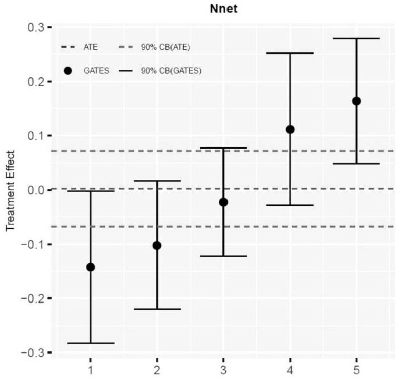
3.2.2. Generic ML analysis. We extend the analysis of HTE conducted in the original paper, by implementing the generic machine learning method developed by Chernozhukov, Demirer et al. (2018). Exploring heterogeneous treatment effects is particularly relevant for this intervention, because a small and insignificant estimate for the ATE could hide significant heterogeneity. Our aim is to dig deeper into the analysis of heterogeneous treatment effects. First, we investigate whether there is significant heterogeneity in treatment effects; second, we analyse whether causal machine learning methods, by implementing a systematic search for heterogeneity across a large number of covariates, can offer additional insights about the characteristics of those who benefited from the programme and those who did not, compared to the traditional methods used in the original paper.

In our analysis, we focus on the main outcome of interest, i.e., student math achievement. Since the results in the original paper are consistently close to zero when comparing the three different treatment arms with the control group, we choose to only analyse one of the treatment arms, corresponding to the PD intervention plus the evaluation. The sample that we use includes 10,006 students in 201 schools. We follow Loyalka et al. (2019a) and cluster standard errors at the school level. In addition to the full set of controls included in the original paper, we also add to our analysis other variables that could be treatment effect modifiers: the baseline values of a

Notes: The estimates are obtained using neural network to produce the proxy predictor . The values reported correspond to the medians over 100 splits.
number of student-level variables, plus variables indicating teachers behaviour in the classroom, evaluated by students at baseline.

The generic method can be used in conjunction with a range of ML tools and Chernozhukov, Demirer et al. (2018) provide two measures-Best BLP and Best GATES to compare the performance of the different ML methods used for the estimation of the proxy predictors. We consider the following methods: elastic net, neural network, and random forest. Based on the results of the Best BLP and Best GATES analysis, reported in Table S3.13 of the Online Appendix, we choose to further work with the neural network.

We first analyse whether overall heterogeneity in treatment effects can be detected. We present results for the best linear predictor (BLP) of the CATE in Table 5. In line with the original paper, the estimated ATE, given by the coefficient , is small (the estimated impact of the PD is 0.002 SD ) and not significantly different from zero. The estimated is instead large and significantly different from zero, which indicates that there is heterogeneity in treatment effects. Next, we estimate the group average treatment effects (GATES). We split the sample into five groups, based on the quintiles of the ML proxy predictor . This analysis reveals further insights into the extent of heterogeneity. Table S3.14 in the Online Appendix reports the GATE in the top and bottom quintile and shows that the GATE in the top quintile is positive, whereas for the bottom quintile the estimated GATE is negative. Both estimates are statistically significant at the level. The difference between the GATE for the top and the bottom quintile is significant, which confirms the presence of heterogeneity in treatment effects. Additionally, Figure 1 reports the GATES estimate and the confidence interval for the five quintiles, as well as for the whole sample (the ATE is represented as a dark dashed line, and the confidence interval as two lighter dashed lines). Notice that for the three middle quintiles the effect of the teacher training intervention is not significantly different from zero.

We then turn to analysing the possible sources of heterogeneity, by implementing the classification analysis (CLAN). Thus, we analyse further the top and bottom quintile in terms of ATE, for which the effect of the PD intervention is positive and negative, respectively. In particular, we compare the student and teacher characteristics in the two groups. As a large number of covariates is available, we focus on the ten covariates for which the correlation with the proxy predictor, , is highest, reported in Table 6. Table S3.15 in the Online Appendix shows the

CLAN analysis for the remaining covariates. Table S3.16 in the Online Appendix reports the correlation for each of the covariates with .

We start by analysing the characteristics of the teachers whose students belong to the least and most affected groups. Interestingly, the variable indicating whether the teacher has a college degree or not is the variable that is most correlated with the proxy predictor, and it was the only one among the variables tested which was found to be a treatment effect modifier across all treatment arms in the original paper. The students in the top quintile are more likely to be taught by a teacher who does not have a college degree, compared to the students in the bottom quintile. This is consistent with the results from Loyalka et al. (2019a), who found that the intervention has a negative effect on students whose teachers have a college degree, but a positive effect on students whose teachers are less qualified. Hence, the PD may help teachers who are less qualified, but, for more qualified teachers, the benefits of the intervention on their students do not outweigh the negative effect of the teachers being absent from the classroom in order to participate in the intervention. Whether or not the teacher majored in math is found to be a potential driver of heterogeneity with the generic method (the results are reported in Table S3.15 in the Online Appendix), whereas in the original paper it was not found to be significant when considering the effect of the PD plus evaluation, which we focus on. The direction of the effect is consistent with what was found in the original analysis: the students in the top quintile are more likely to have been taught by a teacher who does not have a major in math, compared to the students in the bottom quintile. It is also interesting to note that the number of hours of

Notes: This table shows the average value of the teacher and student characteristics for the most and least affected groups. The estimates are obtained using neural network to produce the proxy predictor confidence intervals are reported in parenthesis. The variables Student math score at baseline and Student baseline math anxiety are normalized. The values reported correspond to the medians over 100 splits.
training that the teacher received prior to the intervention, which is not found to be a determinant of heterogeneity in the original paper, is higher in the most affected group compared to the least affected group. This may reflect the fact that teachers who have had more training in the past may be able to better implement the suggestions from the PD intervention. Table 6 shows that teacher rank, experience, and age are higher in the most affected group compared to the least affected group. This is consistent with the existence of a similar mechanism: teachers who have more experience may be able to better implement the suggestions from the PD intervention. As the PD is mainly theoretical, having had other types of training, or having more experience, may be helpful for an effective implementation of the practices learned during the PD.

We then examine whether any of the student characteristics are potential drivers of heterogeneity. In contrast to the findings in Loyalka et al. (2019a), who did not find heterogeneity in terms of student features, we find that students in the most affected group differ in terms of several characteristics compared to students in the least affected group. Among the most correlated with the heterogeneity score (listed in Table 6) are student age and gender: students in the most affected group are on average about half a year older than students in the least affected group,

and the most affected group includes a larger share of male students. Additionally, students in the most affected group, on average, have a lower baseline math score, and tend to be more anxious about math. Thus, teacher PD could be more beneficial for weaker students, and for students who are more anxious about the subject. Finally, class size appears to be a possible determinant of heterogeneity: students who benefit more from the PD tend to be in smaller classes. This result suggests that in smaller classes it may be easier for teachers to implement some of the practices introduced during the PD training. For instance, Loyalka et al. (2019a) mention having students work together in small groups as one of the techniques that were suggested in the PD; this technique is likely to be easier to implement in smaller classes.

In conclusion, our analysis confirms the presence of heterogeneous effects of the teacher PD intervention, and uncovers a rich set of potential determinants of heterogeneity. With the GATES analysis, we are able to show that the achievement of students belonging to the bottom quintile is negatively affected by the intervention, while the achievement of students in the top quintile is positively affected by the intervention. This confirms what was suggested by Loyalka et al. (2019a): that there is a group of students who benefits from the intervention, and a group who does not. In addition, the GATES analysis shows that the effect is not significantly different from zero for the students belonging to the middle quintiles. With the CLAN analysis, we can obtain a clearer picture of the characteristics of the groups who benefit and who do not from the intervention, compared to the original HTE analysis. In line with Loyalka et al. (2019a), we find that teacher characteristics such as having a college degree or having a major in math are potential determinants of heterogeneity. However, our study uncovers additional differences (that were not identified in the original paper) between the least and the most affected groups, in terms of both teacher and student characteristics, such as teacher’s rank, experience, age, and number of training hours, as well as student’s gender, age, baseline math score, baseline math anxiety, and class size.

Our main message is that appropriately combining predictive methods with causal questions adds value to traditional methods and should be more often explored in applied research. We argue that in each revisited study the researcher would have benefited from employing causal ML methods and would have gained additional insights not provided by standard causal inference tools.

We offer the following recommendations for applied researchers about the usefulness of causal ML methods.
(a) Causal ML methods are useful in settings with many potential confounders relative to the sample size. With our revisited examples, we show the importance of taking into account all potentially relevant confounders at once, both linearly and nonlinearly. We revisit the most complete robustness checks of Djankov et al. (2010a) and Nunn and Trefler (2010a), considering all potential confounders linearly and nonlinearly, which would not be possible with traditional methods. Furthermore, our results from the Monte Carlo study suggest that, as the number of covariates used in the estimation increases relative to the sample size, the gains from using DML over OLS increase.
(b) Causal ML methods are more suitable than traditional methods to flexibly capture the effect of covariates. As the true functional form is unknown, with flexible estimation we can better capture the effect of confounders. For instance, when revisiting the results of

Djankov et al. (2010a), we show suggestive evidence that there exist relevant nonlinear terms, which were not taken into account in the original analysis, but are captured by the DML estimation. Moreover, we show with our MC simulations that in the presence of nonlinear confounders DML outperforms OLS.
(c) We further recommend using causal ML methods in settings where the researcher does not have a lot of guidance from theory on which covariates should be included. This is because they implement a systematic model selection, rather than choosing an ad hoc specification, as we discuss when revisiting the results of Djankov et al. (2010a). This argument is also important when performing sensitivity analysis and robustness checks, as highlighted by our results when revisiting Nunn and Trefler (2010a).
(d) Finally, if the researcher is interested in HTE, causal machine learning methods can ensure that relevant heterogeneity and its determinants are not missed, or falsely discovered due to multiple hypothesis testing issues. For example, our analysis of the HTEs of the papers by DellaVigna and Kaplan (2007a) and Loyalka et al. (2019a) reveals potential determinants of heterogeneity that were not considered in the original analyses, which rely on traditional methods. Moreover, causal ML methods can be used to uncover heterogeneity ex post, without being bound to explore HTE only for the specific subgroups indicated in the pre-analysis plan.

These advantages are particularly important in the context of observational studies, where causal ML methods can improve the credibility of causal analysis by making the unconfoundedness assumption more plausible. However, even if the empirical study is a randomized control trial and controlling for confounding factors is not necessarily needed, the use of causal machine learning methods can improve efficiency and provide more precise estimates with lower standard errors and tighter confidence intervals.

Baiardi acknowledges support from EU Horizon 2020, Marie Skłodowska-Curie individual grant (No. 840319). Naghi acknowledges support from EU Horizon 2020, Marie Skłodowska-Curie individual grant (No. 797286). Financial support from the United Nations Sustainable Development Funds is also gratefully acknowledged. We thank participants at the Machine Learning for Economics Workshop (at Barcelona GSE Summer Forum 2019), the Netherlands Econometrics Study Group Meeting 2020, and seminar participants at University of Amsterdam, Etla Economics Research, IMT Lucca and Wageningen University for very helpful comments. Nadja van’t Hoff, Olivier Mulkin, and Christian Wirths provided excellent research assistance.

Athey, S. and G. W. Imbens (2016). Recursive partitioning for heterogeneous causal effects. Proceedings of the National Academy of Sciences 113, 7353-60.
Athey, S. and G. W. Imbens (2017). The state of applied econometrics: Causality and policy evaluation. Journal of Economic Perspectives 31(2), 3-32.
Athey, S. and G. W. Imbens (2019). Machine learning methods that economists should know about. Annual Review of Economics 11, 685-725.

Athey, S., G. W. Imbens and S. Wager (2018). Approximate residual balancing: Debiased inference of average treatment effects in high dimensions. Journal of the Royal Statistical Society: Series B (Statistical Methodology) 80, 597-623.
Athey, S., J. Tibshirani and S. Wager (2019). Generalized random forests. Annals of Statistics 47, 1148-78.
Athey, S. and S. Wager (2019). Estimating treatment effects with causal forests: An application. Observational Studies 5, 37-51.
Bertrand, M., B. Crépon, A. Marguerie and P. Premand (2017). Contemporaneous and post-program impacts of a public works program: Evidence from Côte d’Ivoire. Working paper, University of Chicago, IL.
Chernozhukov, V., D. Chetverikov, M. Demirer, E. Duflo, C. Hansen and W. Newey (2017). Double/debiased/neyman machine learning of treatment effects. American Economic Review 107(5), 261-5.
Chernozhukov, V., D. Chetverikov, M. Demirer, E. Duflo, C. Hansen, W. Newey and J. Robins (2018). Double/debiased machine learning for treatment and structural parameters. Econometrics Journal 21, C1-68.
Chernozhukov, V., M. Demirer, E. Duflo and I. Fernandez-Val (2018). Generic machine learning inference on heterogenous treatment effects in randomized experiments. Working Paper 24678, National Bureau of Economic Research, Cambridge, MA.
Colangelo, K. and Y.-Y. Lee (2020). Double debiased machine learning nonparametric inference with continuous treatments. arXiv: Econometrics 2004.03036.
Davis, J. M. and S. B. Heller (2017). Using causal forests to predict treatment heterogeneity: An application to summer jobs. American Economic Review 107(5), 546-50.
Davis, J. M. and S. B. Heller (2020). Rethinking the benefits of youth employment programs: The heterogeneous effects of summer jobs. Review of Economics and Statistics 102, 664-77.
DellaVigna, S. and E. Kaplan (2007a). The Fox News effect: Media bias and voting. Quarterly Journal of Economics 122, 1187-234.
DellaVigna, S. and E. Kaplan (2007b). The Fox News effect: Media bias and voting [data]. Quarterly Journal of Economics. Data available at. https://eml.berkeley.edu/ sdellavi/index.html.
Deryugina, T., G. Heutel, N. H. Miller, D. Molitor. and J. Reif (2019). The mortality and medical costs of air pollution: Evidence from changes in wind direction. American Economic Review 109(12), 4178-219.
Djankov, S., T. Ganser, C. McLiesh, R. Ramalho and A. Shleifer (2010a). The effect of corporate taxes on investment and entrepreneurship. American Economic Journal: Macroeconomics 2, 31-64.
Djankov, S., T. Ganser, C. McLiesh, R. Ramalho and A. Shleifer (2010b). The effect of corporate taxes on investment and entrepreneurship [data]. American Economic Journal: Macroeconomics. Data deposited at ICPSR, https://www.openicpsr.org/openicpsr/project/114179/version/V1/view.
Fair, R. C. (1978). The effect of economic events on votes for president. Review of Economics and Statistics 60, 159-73.
Farrell, M. H., T. Liang and S. Misra (2021). Deep neural networks for estimation and inference. Econometrica 89, 181-213.
Grossman, G. M. and E. Helpman (1991). Innovation and Growth in the Global Economy. Cambridge, MA: MIT Press.
Hill, J. L. (2011). Bayesian nonparametric modeling for causal inference. Journal of Computational and Graphical Statistics 20, 217-40.
Imai, K. and M. Ratkovic (2013). Estimating treatment effect heterogeneity in randomized program evaluation. Annals of Applied Statistics 7, 443-70.
Imbens, G. W. and D. B. Rubin (2015). Causal Inference in Statistics, Social, and Biomedical Sciences. New York: Cambridge University Press.

Imbens, G. W. and J. M. Wooldridge (2009). Recent developments in the econometrics of program evaluation. Journal of Economic Literature 47, 5-86.
Knaus, M. C., M. Lechner and A. Strittmatter (2022). Heterogeneous employment effects of job search programmes: A machine learning approach. Journal of Human Resources 57, 597-636.
Kramer, G. H. (1971). Short-term fluctuations in us voting behavior, 1896-1964. American Political Science Review 65, 131-43.
Lewis-Beck, M. S. and M. Stegmaier (2000). Economic determinants of electoral outcomes. Annual Review of Political Science 3, 183-219.
List, J. A., A. M. Shaikh and Y. Xu (2019). Multiple hypothesis testing in experimental economics. Experimental Economics 22, 773-93.
Loyalka, P., A. Popova, G. Li and Z. Shi (2019a). Does teacher training actually work? Evidence from a large-scale randomized evaluation of a national teacher training program. American Economic Journal: Applied Economics 11, 128-54.
Loyalka, P., A. Popova, G. Li and Z. Shi (2019b). Does teacher training actually work? Evidence from a large-scale randomized evaluation of a national teacher training program [data]. American Economic Journal: Applied Economics. Data deposited at ICPSR, https://www.openicpsr.org/openicpsr/project/11 6356/version/V1/view.
Nunn, N. and D. Trefler (2010a). The structure of tariffs and long-term growth. American Economic Journal: Macroeconomics 2, 158-94.
Nunn, N. and D. Trefler (2010b). The structure of tariffs and long-term growth [data]. American Economic Journal: Macroeconomics. Data deposited at ICPSR, https://www.openicpsr.org/openicpsr/project/1141 83/version/V1/view.
Oprescu, M., V. Syrgkanis and Z. S. Wu (2019). Orthogonal random forest for causal inference. Proceedings of the 36th International Conference on Machine Learning PMLR 97, 4932-41.
Pissarides, C. A. (1980). British government popularity and economic performance. Economic Journal 90, 569-81.
Semenova, V., M. Goldman, V. Chernozhukov and M. Taddy (2018). Orthogonal machine learning for demand estimation: High dimensional causal inference in dynamic panels. arXiv: Machine Learning 1712.09988.

Strittmatter, A. (2019). What is the value added by using causal machine learning methods in a welfare experiment evaluation? Working paper, Global Labor Organization, Essen, Germany.
Su, X., C.-L. Tsai, H. Wang, D. M. Nickerson and B. Li (2009). Subgroup analysis via recursive partitioning. Journal of Machine Learning Research 10, 141-58.
Van der Laan, M. J. and S. Rose (2011). Targeted Learning: Causal Inference for Observational and Experimental Data. New York: Springer Science and Business Media.
Wager, S. and S. Athey (2018). Estimation and inference of heterogeneous treatment effects using random forests. Journal of the American Statistical Association 113, 1228-42.
Zeileis, A., T. Hothorn and K. Hornik (2008). Model-based recursive partitioning. Journal of Computational and Graphical Statistics 17, 492-514.

Additional Supporting Information may be found in the online version of this article at the publisher’s website:

Online Appendix
Replication Package
Co-editor Victor Chernozhukov handled this manuscript.