DOI: https://doi.org/10.64389/mjs.2025.01111
تاريخ النشر: 2025-07-12
مقالة بحثية
مقدرات ليو المعدلة الجديدة للتعامل مع التعدد الخطي في نموذج الانحدار بيتا: المحاكاة والتطبيقات
معلومات المقال
الكلمات المفتاحية:
مقدّر ليو المعدل
التعدد الخطي
مقدرات متحيزة
مقدّر ريدج
تصنيف موضوع الرياضيات:
التواريخ المهمة:
تاريخ المراجعة: 7 يوليو 2025
تاريخ القبول: 10 يوليو 2025
تاريخ النشر على الإنترنت: 12 يوليو 2025
الملخص
نموذج الانحدار بيتا (BRM) يُستخدم على نطاق واسع لتحليل المتغيرات المستجيبة المحدودة، مثل النسب والنسب المئوية. ومع ذلك، عندما يوجد تعدد خطي بين المتغيرات التفسيرية، يصبح مقدر الاحتمالية القصوى التقليدي (MLE) غير مستقر وغير فعال. لمعالجة هذه المشكلة، نقترح مقدرات ليو المعدلة الجديدة لـ BRM، المصممة لتعزيز دقة التقدير في وجود تعدد خطي مرتفع بين المتنبئين. تمتد المقدرات المقترحة مقدر ليو التقليدي من خلال دمج معلمات تحيز مرنة، مما يوفر بديلاً أكثر قوة لـ MLE. تُظهر المقارنات النظرية تفوق المقدرات الجديدة على الطرق الحالية. بالإضافة إلى ذلك، تُظهر محاكاة مونت كارلو والتطبيقات الواقعية أدائها المحسن من حيث متوسط الخطأ التربيعي (MSE) ومتوسط الخطأ المطلق (MAE). تشير النتائج إلى أن المقدرات المقترحة تقلل بشكل كبير من تحيز التقدير والتباين تحت التعدد الخطي، مما يوفر معاملات انحدار أكثر موثوقية.
1. المقدمة
أن هذه المقدرات ذات المعاملين تؤدي أداءً أفضل من البدائل ذات المعامل الواحد. بناءً على هذه الأسس، اقترحت الدراسة الحالية معلمات ليو المعدلة لـ BRM. نقترح مقدر ليو المعدل الجديد ذو المعامل الواحد والمعاملين المصمم خصيصًا لتقليل آثار التعدد الخطي في BRM. نقدم طرقًا منهجية لاختيار المعلمات المثلى ونقوم بإجراء مقارنات أداء مفصلة باستخدام المحاكاة والتطبيقات مع الطرق الحالية، بما في ذلك MLE، ريدج، ومقدرات ليو.
2. المنهجية
لمعالجة تحديات التعدد الخطي في نماذج الانحدار المتعدد، اقترح كارلسون وآخرون [23] مقدر بيتا ليو (BLE)، موضحين أدائه المتفوق مقارنةً بنموذج الانحدار التقليدي. يتم تعريف BLE رسميًا على النحو التالي:
- في
، يصبح تقدير الاحتمال البايزي (BLE) هو تقدير الاحتمال الأقصى (MLE). - لـ
يُنتج BLE معاملات متقلصة، مما يخفف بشكل فعال من آثار التعدد الخطي.
3. المقترحات المقدمة للمقدرات
3.1. مُقدِّر ليو المعدل ببارامتر واحد بيتا
3.2. مُقدِّر ليو ذو المعلمتين المعدل بيتا
3.3. المقارنة النظرية باستخدام MMSE و MSE القياسي
العبارة 1. لأي مصفوفة إيجابية محددة
برهان:
النظرية 2. MMSE
برهان:
النظرية 3. MMSE
برهان:
نظرية 4.
برهان:
3.4. اختيار معلمة التحيز
4. محاكاة مونت كارلو
|
|
ن | BRRE | BLE | بي إم أو بي إل إي | BMTPLE | |||||||
| MLE |
|
|
|
|
|
|
|
|
|
|||
| 0.80 | 30 | 0.59865 | 0.54371 | 0.49854 | 0.56211 | 0.39102 | 0.39102 | 0.37994 | 0.33192 | 0.20262 | 0.34711 | 0.28845 |
| 75 | 0.19933 | 0.19256 | 0.18632 | 0.19933 | 0.17260 | 0.17260 | 0.16869 | 0.15986 | 0.09519 | 0.16513 | 0.15060 | |
| 150 | 0.11661 | 0.11402 | 0.11265 | 0.11661 | 0.10658 | 0.10658 | 0.10331 | 0.09981 | 0.08418 | 0.10228 | 0.09610 | |
| ٢٠٠ | 0.11329 | 0.11116 | 0.10977 | 0.11329 | 0.10491 | 0.10491 | 0.10251 | 0.09944 | 0.07102 | 0.10162 | 0.09612 | |
| ٣٠٠ | 0.09902 | 0.09755 | 0.09668 | 0.09902 | 0.09322 | 0.09322 | 0.09092 | 0.08876 | 0.06318 | 0.09028 | 0.08641 | |
| ٤٠٠ | 0.06504 | 0.06430 | 0.06370 | 0.06504 | 0.06210 | 0.06210 | 0.06054 | 0.05951 | 0.05806 | 0.06027 | 0.05837 | |
| 0.85 | 30 | 0.84338 | 0.76349 | 0.71370 | 0.73158 | 0.52125 | 0.52125 | 0.49182 | 0.42789 | 0.24850 | 0.43504 | 0.36954 |
| 75 | 0.30541 | 0.29075 | 0.27662 | 0.30094 | 0.24410 | 0.24410 | 0.23899 | 0.22051 | 0.13431 | 0.23153 | 0.20178 | |
| 150 | 0.20878 | 0.20105 | 0.19498 | 0.20878 | 0.17764 | 0.17764 | 0.17393 | 0.16354 | 0.09076 | 0.17027 | 0.15263 | |
| ٢٠٠ | 0.12849 | 0.12535 | 0.12227 | 0.12849 | 0.11648 | 0.11648 | 0.11359 | 0.10901 | 0.06146 | 0.11215 | 0.10409 | |
| ٣٠٠ | 0.11050 | 0.10836 | 0.10621 | 0.11050 | 0.10211 | 0.10211 | 0.09953 | 0.09637 | 0.05833 | 0.09861 | 0.09294 | |
| ٤٠٠ | 0.10401 | 0.10245 | 0.10122 | 0.10401 | 0.09716 | 0.09716 | 0.09518 | 0.09275 | 0.06649 | 0.09466 | 0.09009 | |
| 0.90 | 30 | 0.97613 | 0.85885 | 0.74545 | 0.71295 | 0.50368 | 0.50368 | 0.48818 | 0.40588 | 0.42283 | 0.42927 | 0.33484 |
| 75 | 0.44011 | 0.40812 | 0.37435 | 0.42929 | 0.30917 | 0.30917 | 0.30259 | 0.26617 | 0.17612 | 0.28607 | 0.23098 | |
| 150 | 0.25209 | 0.24082 | 0.23379 | 0.25209 | 0.20571 | 0.20571 | 0.20091 | 0.18573 | 0.10259 | 0.19494 | 0.17021 | |
| ٢٠٠ | 0.15451 | 0.14963 | 0.14485 | 0.15451 | 0.13449 | 0.13449 | 0.13113 | 0.12405 | 0.04949 | 0.12798 | 0.11656 | |
| ٣٠٠ | 0.17619 | 0.17159 | 0.16822 | 0.17619 | 0.15751 | 0.15751 | 0.15411 | 0.14728 | 0.08178 | 0.15207 | 0.13996 | |
| ٤٠٠ | 0.12033 | 0.11756 | 0.11509 | 0.12033 | 0.10948 | 0.10948 | 0.10656 | 0.10225 | 0.05919 | 0.10534 | 0.09764 | |
| 0.95 | 30 | 1.95145 | 1.61153 | 1.33847 | 0.74971 | 0.63125 | 0.63125 | 0.60304 | 0.46309 | 0.75117 | 0.46704 | 0.36082 |
| 75 | 0.77058 | 0.68403 | 0.59467 | 0.67190 | 0.40887 | 0.40887 | 0.39664 | 0.32293 | 0.29066 | 0.34976 | 0.25791 | |
| 150 | 0.65448 | 0.61273 | 0.57333 | 0.46494 | 0.40631 | 0.40631 | 0.39867 | 0.35792 | 0.26362 | 0.37198 | 0.31806 | |
| ٢٠٠ | 0.46969 | 0.44678 | 0.43155 | 0.39893 | 0.33836 | 0.33836 | 0.33232 | 0.30280 | 0.20512 | 0.31955 | 0.27328 | |
| ٣٠٠ | 0.30380 | 0.28634 | 0.26932 | 0.30325 | 0.23318 | 0.23318 | 0.22857 | 0.20623 | 0.09539 | 0.21881 | 0.18363 | |
| ٤٠٠ | 0.24916 | 0.23768 | 0.22492 | 0.24784 | 0.20084 | 0.20084 | 0.19702 | 0.18129 | 0.09088 | 0.19109 | 0.16502 | |
| 0.99 | 30 | ١٤.١٤٤٤٤ | 10.76913 | 9.79942 | 1.91565 | 0.41671 | 0.41671 | 0.38925 | 0.27750 | ٢.٣١٢١٨ | 0.16890 | 0.22069 |
| 75 | 3.78885 | ٣.٠٢٧٣٧ | 2.62939 | 0.37407 | 0.53995 | 0.53995 | 0.50980 | 0.34694 | 1.03086 | 0.26050 | 0.24739 | |
| 150 | ٢.٢٩٢٧٤ | 1.84316 | 1.52954 | 0.57198 | 0.48478 | 0.48478 | 0.45777 | 0.30119 | 0.79692 | 0.29312 | 0.19747 | |
| ٢٠٠ | 1.70053 | 1.41316 | 1.18927 | 0.70098 | 0.49920 | 0.49920 | 0.47538 | 0.33489 | 0.64845 | 0.35025 | 0.23149 | |
| ٣٠٠ | 1.34593 | 1.15361 | 0.98523 | 0.75240 | 0.48773 | 0.48773 | 0.46838 | 0.34919 | 0.63455 | 0.38140 | 0.25647 | |
| ٤٠٠ | 1.06164 | 0.90709 | 0.76542 | 0.74014 | 0.42958 | 0.42958 | 0.41236 | 0.30474 | 0.42084 | 0.33755 | 0.21832 | |
|
|
ن | BRRE | BLE | بي إم أو بي إل إي | BMTPLE | |||||||
| MLE |
|
|
|
|
|
|
|
|
|
|||
| 0.80 | 30 | 0.64750 | 0.52111 | 0.42427 | 0.45862 | 0.45128 | 0.40733 | 0.41213 | 0.38837 | 0.16780 | 0.38943 | 0.35503 |
| 75 | 0.15702 | 0.14471 | 0.13449 | 0.15652 | 0.14051 | 0.13388 | 0.12976 | 0.12605 | 0.06906 | 0.12810 | 0.12061 | |
| 150 | 0.09021 | 0.08601 | 0.08350 | 0.09021 | 0.08440 | 0.08332 | 0.07876 | 0.07751 | 0.07712 | 0.07827 | 0.07564 | |
| ٢٠٠ | 0.08276 | 0.07930 | 0.07664 | 0.08276 | 0.07808 | 0.07656 | 0.07295 | 0.07186 | 0.05689 | 0.07260 | 0.07017 | |
| ٣٠٠ | 0.07660 | 0.07372 | 0.07153 | 0.07660 | 0.07262 | 0.07149 | 0.06802 | 0.06704 | 0.04608 | 0.06769 | 0.06554 | |
| ٤٠٠ | 0.04074 | 0.03973 | 0.03887 | 0.04074 | 0.03938 | 0.03885 | 0.03680 | 0.03649 | 0.04957 | 0.03668 | 0.03601 | |
| 0.85 | 30 | 0.56840 | 0.44911 | 0.38988 | 0.42134 | 0.38533 | 0.37133 | 0.32529 | 0.30210 | 0.12344 | 0.29520 | 0.27365 |
| 75 | 0.21368 | 0.18830 | 0.16699 | 0.20885 | 0.17881 | 0.16503 | 0.16601 | 0.15803 | 0.05910 | 0.16179 | 0.14713 | |
| 150 | 0.15136 | 0.13888 | 0.12834 | 0.14881 | 0.13404 | 0.12771 | 0.12515 | 0.12109 | 0.05286 | 0.12348 | 0.11523 | |
| ٢٠٠ | 0.09343 | 0.08869 | 0.08489 | 0.09343 | 0.08696 | 0.08478 | 0.08055 | 0.07892 | 0.04151 | 0.07996 | 0.07648 | |
| ٣٠٠ | 0.08379 | 0.07984 | 0.07630 | 0.08379 | 0.07835 | 0.07620 | 0.07292 | 0.07153 | 0.03097 | 0.07235 | 0.06944 | |
| ٤٠٠ | 0.06466 | 0.06230 | 0.06021 | 0.06466 | 0.06149 | 0.06016 | 0.05690 | 0.05612 | 0.03517 | 0.05666 | 0.05490 | |
| 0.90 | 30 | 0.83745 | 0.61988 | 0.46531 | 0.46258 | 0.48474 | 0.42572 | 0.43904 | 0.39826 | 0.17644 | 0.39233 | 0.35028 |
| 75 | 0.39174 | 0.32949 | 0.27112 | 0.33751 | 0.29292 | 0.26584 | 0.27448 | 0.25572 | 0.09356 | 0.26294 | 0.23160 | |
| 150 | 0.17707 | 0.15849 | 0.14698 | 0.17696 | 0.15092 | 0.14570 | 0.13695 | 0.13083 | 0.04159 | 0.13374 | 0.12243 | |
| ٢٠٠ | 0.12556 | 0.11622 | 0.10920 | 0.12541 | 0.11262 | 0.10893 | 0.10354 | 0.10031 | 0.03265 | 0.10212 | 0.09563 | |
| ٣٠٠ | 0.09785 | 0.09181 | 0.08699 | 0.09785 | 0.08955 | 0.08680 | 0.08262 | 0.08047 | 0.02875 | 0.08167 | 0.07733 | |
| ٤٠٠ | 0.08634 | 0.08165 | 0.07753 | 0.08634 | 0.07989 | 0.07738 | 0.07356 | 0.07187 | 0.02584 | 0.07289 | 0.06935 | |
| 0.95 | 30 | 1.68443 | 1.09561 | 0.77204 | 0.48652 | 0.68062 | 0.62751 | 0.57881 | 0.50033 | 0.32582 | 0.44611 | 0.42852 |
| 75 | 0.73111 | 0.54663 | 0.39375 | 0.47995 | 0.43239 | 0.36634 | 0.39682 | 0.35168 | 0.12190 | 0.35665 | 0.30196 | |
| 150 | 0.37054 | 0.30386 | 0.24197 | 0.31657 | 0.26622 | 0.23681 | 0.24696 | 0.22742 | 0.07983 | 0.23379 | 0.20314 | |
| ٢٠٠ | 0.27551 | 0.23754 | 0.21064 | 0.26342 | 0.21795 | 0.20874 | 0.19910 | 0.18651 | 0.05127 | 0.19220 | 0.17011 | |
| ٣٠٠ | 0.25655 | 0.22332 | 0.19001 | 0.24689 | 0.20769 | 0.18726 | 0.19444 | 0.18341 | 0.04651 | 0.18890 | 0.16850 | |
| ٤٠٠ | 0.18348 | 0.16438 | 0.14629 | 0.17802 | 0.15497 | 0.14527 | 0.14403 | 0.13731 | 0.03603 | 0.14085 | 0.12803 | |
| 0.99 | 30 | 6.93854 | 2.90235 | ٢.٢٦٣٨٤ | 0.86870 | 0.32289 | 0.31842 | 0.21776 | 0.15566 | 0.44098 | 0.16182 | 0.13505 |
| 75 | ٢.٩١٤٢٤ | 1.59392 | 1.11270 | 0.18493 | 0.51965 | 0.49462 | 0.41557 | 0.30699 | 0.41887 | 0.19873 | 0.24476 | |
| 150 | ٢.١٦٣٧٥ | 1.39194 | 1.02453 | 0.29387 | 0.57347 | 0.52891 | 0.48072 | 0.37903 | 0.35615 | 0.30998 | 0.30361 | |
| ٢٠٠ | 1.52260 | 1.01553 | 0.71168 | 0.39518 | 0.54538 | 0.49432 | 0.47786 | 0.39059 | 0.31249 | 0.36324 | 0.31620 | |
| ٣٠٠ | 1.28047 | 0.88479 | 0.59777 | 0.48224 | 0.54690 | 0.48200 | 0.48736 | 0.40500 | 0.25899 | 0.39680 | 0.33012 | |
| ٤٠٠ | 0.98168 | 0.69490 | 0.48538 | 0.47849 | 0.47422 | 0.41223 | 0.42778 | 0.36201 | 0.18815 | 0.36141 | 0.29878 | |
ال
5. التطبيقات
|
|
ن | BRRE | BLE | BMTPLE | ||||||||
| MLE |
|
|
|
|
بي إم أو بي إل إي |
|
|
|
|
|
||
| 0.80 | 30 | 2.64169 | 2.40458 | ٢.١٠٦٥٠ | 1.77960 | 1.33606 | 1.33567 | 1.29169 | 1.14548 | 0.45200 | 0.99216 | 0.80629 |
| 75 | 1.10480 | 1.07215 | 1.04870 | 0.65330 | 0.64745 | 0.64745 | 0.60047 | 0.56443 | 0.16792 | 0.51434 | 0.46595 | |
| 150 | 0.47603 | 0.46338 | 0.45160 | 0.46713 | 0.41723 | 0.41720 | 0.39379 | 0.37521 | 0.11558 | 0.37783 | 0.32299 | |
| ٢٠٠ | 0.33721 | 0.33028 | 0.32274 | 0.33721 | 0.30710 | 0.30710 | 0.28923 | 0.27844 | 0.07285 | 0.28030 | 0.24701 | |
| ٣٠٠ | 0.31110 | 0.30516 | 0.30200 | 0.28159 | 0.27915 | 0.27915 | 0.25681 | 0.24986 | 0.08806 | 0.24978 | 0.22903 | |
| ٤٠٠ | 0.28495 | 0.28147 | 0.27930 | 0.28080 | 0.26548 | 0.26548 | 0.25224 | 0.24652 | 0.08035 | 0.24759 | 0.22935 | |
| 0.85 | 30 | 2.87692 | 2.63193 | 2.33615 | 1.87831 | 1.31017 | 1.30979 | 1.24291 | 1.08697 | 0.40597 | 0.92900 | 0.73996 |
| 75 | 1.08265 | 1.03854 | 0.99123 | 0.91909 | 0.78523 | 0.78523 | 0.75382 | 0.70133 | 0.14955 | 0.67579 | 0.56095 | |
| 150 | 0.53274 | 0.51535 | 0.50001 | 0.53274 | 0.45060 | 0.45060 | 0.42550 | 0.40029 | 0.10548 | 0.40236 | 0.33068 | |
| ٢٠٠ | 0.39951 | 0.38841 | 0.37884 | 0.39951 | 0.35090 | 0.35090 | 0.32722 | 0.31093 | 0.06772 | 0.31213 | 0.26458 | |
| ٣٠٠ | 0.44089 | 0.43337 | 0.42737 | 0.39901 | 0.38634 | 0.38634 | 0.36734 | 0.35644 | 0.09867 | 0.35664 | 0.32423 | |
| ٤٠٠ | 0.24624 | 0.24185 | 0.23885 | 0.24624 | 0.22792 | 0.22792 | 0.21241 | 0.20523 | 0.04804 | 0.20649 | 0.18411 | |
| 0.90 | 30 | ٤.٤٨٤٦٢ | 3.90853 | 3.34183 | 1.76829 | 1.52439 | 1.52439 | 1.48083 | 1.25481 | 0.83019 | 0.89733 | 0.82254 |
| 75 | 1.57276 | 1.47943 | 1.32581 | 1.50402 | 1.06089 | 1.06089 | 1.02829 | 0.92375 | 0.28273 | 0.89047 | 0.66320 | |
| 150 | 0.76350 | 0.72929 | 0.69584 | 0.76350 | 0.59480 | 0.59480 | 0.56200 | 0.51623 | 0.10481 | 0.51124 | 0.39543 | |
| ٢٠٠ | 0.66836 | 0.64669 | 0.62930 | 0.61539 | 0.54225 | 0.54225 | 0.50468 | 0.47474 | 0.08066 | 0.46773 | 0.39156 | |
| ٣٠٠ | 0.65632 | 0.64172 | 0.62826 | 0.59069 | 0.54129 | 0.54129 | 0.51659 | 0.49443 | 0.13431 | 0.49182 | 0.43091 | |
| ٤٠٠ | 0.40050 | 0.39055 | 0.38242 | 0.40050 | 0.35514 | 0.35514 | 0.33309 | 0.31729 | 0.05772 | 0.31926 | 0.27206 | |
| 0.95 | 30 | 8.66006 | 7.30329 | 6.04024 | 1.49363 | 1.63259 | 1.63259 | 1.59365 | 1.31432 | 0.98935 | 0.56670 | 0.81276 |
| 75 | ٢.٤٣٢٣٨ | ٢.٢٢٣٤٤ | 1.93829 | 2.07747 | 1.24529 | 1.24529 | 1.21509 | 1.04092 | 0.39006 | 0.90334 | 0.65857 | |
| 150 | 1.79797 | 1.66360 | 1.47969 | 1.71622 | 1.06254 | 1.06254 | 1.03175 | 0.89822 | 0.29090 | 0.82312 | 0.58913 | |
| ٢٠٠ | 1.26987 | 1.19753 | 1.09461 | 1.24894 | 0.88111 | 0.88111 | 0.84936 | 0.76029 | 0.15425 | 0.73623 | 0.53766 | |
| ٣٠٠ | 0.87923 | 0.83916 | 0.79237 | 0.86756 | 0.66557 | 0.66557 | 0.63796 | 0.58192 | 0.11254 | 0.57548 | 0.43693 | |
| ٤٠٠ | ٢.٤٠٣٣٣ | ٢.٣٤١٧٢ | ٢.٣٠٦٥١ | 1.08319 | 0.98300 | 0.98300 | 0.91888 | 0.86690 | 0.11773 | 0.75832 | 0.72395 | |
| 0.99 | 30 | ٤٦.٥٣٢٦٧ | ٣٩.١٣٦٥٣ | 33.84793 | ٤.٥٦٣٦٥ | 1.02191 | 1.02191 | 1.00490 | 0.82855 | 3.30725 | ٢.٥٣٣٥٢ | 0.53972 |
| 75 | 14.31168 | 12.59060 | 10.78966 | 1.09636 | 1.51731 | 1.51731 | 1.49352 | 1.19007 | 1.50903 | 0.26156 | 0.65130 | |
| 150 | 8.56375 | 7.60768 | 6.50498 | 1.79189 | 1.48829 | 1.48829 | 1.46132 | 1.15434 | 1.17424 | 0.45137 | 0.61263 | |
| ٢٠٠ | 5.91519 | 5.27114 | ٤.٤٧٠٠٢ | 2.37686 | 1.52570 | 1.52570 | 1.50343 | 1.19409 | 0.65663 | 0.65281 | 0.60015 | |
| ٣٠٠ | ٤.٥٢٥٩٥ | ٤.٠٨٠٠٥ | 3.41682 | 2.63069 | 1.53344 | 1.53327 | 1.58315 | 1.23394 | 0.75394 | 0.87444 | 0.67794 | |
| ٤٠٠ | 5.78554 | 5.40341 | ٤.٨٩١٢٤ | ٢.٧٦٠٢٦ | 1.70205 | 1.70205 | 1.67444 | 1.41825 | 0.64502 | 0.98075 | 0.88845 | |
|
|
ن | BRRE | BLE | BMTPLE | ||||||||
| MLE |
|
|
|
|
بي إم أو بي إل إي |
|
|
|
|
|
||
| 0.80 | 30 | 1.83877 | 1.44699 | 1.06422 | 1.18693 | 1.14327 | 0.97437 | 1.01112 | 0.92170 | 0.30634 | 0.77951 | 0.71436 |
| 75 | 0.57997 | 0.53073 | 0.47991 | 0.54481 | 0.49251 | 0.46933 | 0.44340 | 0.42461 | 0.09565 | 0.41621 | 0.36792 | |
| 150 | 0.30259 | 0.28380 | 0.26640 | 0.30167 | 0.27454 | 0.26559 | 0.24252 | 0.23418 | 0.06719 | 0.23253 | 0.20836 | |
| ٢٠٠ | 0.22476 | 0.21404 | 0.20312 | 0.22476 | 0.20937 | 0.20280 | 0.18487 | 0.18010 | 0.05297 | 0.17933 | 0.16465 | |
| ٣٠٠ | 0.21275 | 0.20346 | 0.19590 | 0.21275 | 0.19948 | 0.19574 | 0.17411 | 0.16995 | 0.04857 | 0.16944 | 0.15625 | |
| ٤٠٠ | 0.14582 | 0.14092 | 0.13678 | 0.14582 | 0.13892 | 0.13671 | 0.12238 | 0.12012 | 0.04721 | 0.12006 | 0.11256 | |
| 0.85 | 30 | 1.82500 | 1.45547 | 1.07658 | 1.18792 | 1.12901 | 1.00693 | 1.01537 | 0.92390 | 0.29687 | 0.78769 | 0.71469 |
| 75 | 0.65561 | 0.58562 | 0.51427 | 0.64153 | 0.53991 | 0.50876 | 0.47695 | 0.45069 | 0.08164 | 0.43515 | 0.37568 | |
| 150 | 0.42016 | 0.38795 | 0.35740 | 0.41946 | 0.37053 | 0.35598 | 0.32902 | 0.31539 | 0.07141 | 0.31158 | 0.27418 | |
| ٢٠٠ | 0.37313 | 0.34939 | 0.32569 | 0.36966 | 0.33489 | 0.32380 | 0.29477 | 0.28452 | 0.04316 | 0.28121 | 0.25220 | |
| ٣٠٠ | 0.23383 | 0.22290 | 0.21314 | 0.23383 | 0.21750 | 0.21286 | 0.19323 | 0.18803 | 0.04010 | 0.18735 | 0.17127 | |
| ٤٠٠ | 0.21292 | 0.20401 | 0.19618 | 0.21292 | 0.19981 | 0.19603 | 0.17672 | 0.17250 | 0.03321 | 0.17197 | 0.15862 | |
| 0.90 | 30 | ٤.٢٦٤٨٨ | ٣.٠٢٣٨٩ | 2.07686 | 1.13010 | 1.65646 | 1.52159 | 1.42122 | 1.27032 | 0.71327 | 0.84827 | 0.97675 |
| 75 | 0.96233 | 0.82457 | 0.64968 | 0.85692 | 0.70945 | 0.62838 | 0.64029 | 0.58953 | 0.13196 | 0.55113 | 0.46057 | |
| 150 | 0.68256 | 0.61024 | 0.53307 | 0.67437 | 0.56186 | 0.52849 | 0.50150 | 0.47141 | 0.07558 | 0.45728 | 0.38752 | |
| ٢٠٠ | 0.48817 | 0.45086 | 0.41836 | 0.45866 | 0.41998 | 0.40534 | 0.37401 | 0.35828 | 0.04965 | 0.35098 | 0.31104 | |
| ٣٠٠ | 0.33067 | 0.30821 | 0.28691 | 0.33067 | 0.29656 | 0.28614 | 0.26091 | 0.25065 | 0.03357 | 0.24815 | 0.21923 | |
| ٤٠٠ | 0.32034 | 0.30122 | 0.28391 | 0.32034 | 0.28935 | 0.28271 | 0.25730 | 0.24801 | 0.03325 | 0.24654 | 0.21915 | |
| 0.95 | 30 | 7.49130 | 5.17984 | ٣.٥٩٢٦٢ | 0.82873 | 1.99582 | 1.93539 | 1.71198 | 1.50775 | 0.71993 | 0.63689 | 1.14818 |
| 75 | 1.85635 | 1.47272 | 1.06156 | 1.24485 | 1.05443 | 0.96045 | 0.96265 | 0.85110 | 0.19345 | 0.69663 | 0.61571 | |
| 150 | 1.52308 | 1.26653 | 0.97146 | 1.18191 | 0.98375 | 0.89465 | 0.89512 | 0.80985 | 0.15599 | 0.70891 | 0.60865 | |
| ٢٠٠ | 1.15016 | 1.01552 | 0.84704 | 0.93563 | 0.82545 | 0.75061 | 0.75308 | 0.70096 | 0.09803 | 0.65054 | 0.56469 | |
| ٣٠٠ | 0.76535 | 0.67981 | 0.57337 | 0.75647 | 0.61234 | 0.56729 | 0.55279 | 0.51534 | 0.05813 | 0.49717 | 0.41425 | |
| ٤٠٠ | 0.59861 | 0.53845 | 0.47632 | 0.59506 | 0.49941 | 0.47339 | 0.44629 | 0.42078 | 0.04042 | 0.40916 | 0.34876 | |
| 0.99 | 30 | ٣٤.٧٢٣٢٤ | 22.88346 | 16.87703 | 7.82112 | 1.20571 | 1.20513 | 1.11674 | 0.95281 | 1.61605 | 2.77552 | 0.74712 |
| 75 | 10.10960 | 6.90541 | ٤.٥٥٠٢٦ | 0.43189 | 1.59396 | 1.58933 | ١.٤٤٤٤٧ | 1.18678 | 0.72038 | 0.21227 | 0.80404 | |
| 150 | 5.68694 | 3.97307 | ٢.٦١٨٦٩ | 0.85581 | 1.38724 | 1.35887 | 1.26837 | 1.02548 | 0.47350 | 0.33012 | 0.66594 | |
| ٢٠٠ | 5.18955 | 3.97351 | ٢.٧٨٣٦٤ | 1.22267 | 1.64480 | 1.59475 | 1.51056 | 1.27291 | 0.33539 | 0.61082 | 0.86192 | |
| ٣٠٠ | 5.04496 | ٤.١٩٩٨٧ | 3.30905 | 1.48063 | 1.82360 | 1.74464 | 1.71323 | 1.50816 | 0.32844 | 0.92600 | 1.11495 | |
| ٤٠٠ | ٣.٠٠٣٨٦ | 2.30031 | 1.54180 | 1.42011 | 1.31878 | 1.24651 | 1.21399 | 1.03222 | 0.25264 | 0.70063 | 0.68973 | |
5.1. مجموعة بيانات نسبة الدهون في الجسم
|
|
ن | BRRE | BLE | بيموبل | BMTPLE | |||||||
| MLE |
|
|
|
|
|
|
|
|
|
|||
| 0.80 | 30 | 1.26890 | 1.21011 | 1.16031 | 1.20732 | 1.03130 | 1.03130 | 1.01514 | 0.95288 | 0.76332 | 0.97479 | 0.89002 |
| 75 | 0.77041 | 0.75887 | 0.74864 | 0.75442 | 0.71742 | 0.71742 | 0.70911 | 0.69288 | 0.49775 | 0.70035 | 0.67491 | |
| 150 | 0.56644 | 0.56054 | 0.55783 | 0.56644 | 0.54263 | 0.54263 | 0.53418 | 0.52629 | 0.47117 | 0.53091 | 0.51789 | |
| ٢٠٠ | 0.52310 | 0.51826 | 0.51524 | 0.52310 | 0.50332 | 0.50332 | 0.49575 | 0.48843 | 0.41674 | 0.49314 | 0.48034 | |
| ٣٠٠ | 0.43000 | 0.42691 | 0.42524 | 0.43000 | 0.41782 | 0.41782 | 0.41142 | 0.40756 | 0.40672 | 0.41009 | 0.40343 | |
| ٤٠٠ | 0.38469 | 0.38281 | 0.38136 | 0.38469 | 0.37719 | 0.37719 | 0.37225 | 0.36990 | 0.38241 | 0.37145 | 0.36739 | |
| 0.85 | 30 | 1.30810 | 1.24576 | 1.20842 | 1.24582 | 1.04219 | 1.04219 | 1.00798 | 0.93671 | 0.71812 | 0.95073 | 0.86658 |
| 75 | 0.83302 | 0.81311 | 0.79574 | 0.83276 | 0.75189 | 0.75189 | 0.74226 | 0.71360 | 0.50549 | 0.72905 | 0.68296 | |
| 150 | 0.68893 | 0.67727 | 0.66926 | 0.68264 | 0.63840 | 0.63840 | 0.63076 | 0.61395 | 0.48316 | 0.62444 | 0.59557 | |
| ٢٠٠ | 0.54907 | 0.54235 | 0.53621 | 0.54907 | 0.52213 | 0.52213 | 0.51180 | 0.50194 | 0.35977 | 0.50785 | 0.49111 | |
| ٣٠٠ | 0.55313 | 0.54809 | 0.54369 | 0.54569 | 0.52959 | 0.52959 | 0.52149 | 0.51393 | 0.38609 | 0.51844 | 0.50570 | |
| ٤٠٠ | 0.42353 | 0.42048 | 0.41842 | 0.42353 | 0.41147 | 0.41147 | 0.40400 | 0.39959 | 0.35302 | 0.40234 | 0.39473 | |
| 0.90 | 30 | 1.50798 | 1.41596 | 1.32717 | 1.38089 | 1.13144 | 1.13144 | 1.11369 | 1.01769 | 0.90307 | 1.04158 | 0.92667 |
| 75 | 1.07544 | 1.03594 | 0.99610 | 1.05919 | 0.90533 | 0.90533 | 0.89427 | 0.84024 | 0.58383 | 0.86522 | 0.78462 | |
| 150 | 0.73651 | 0.72044 | 0.71134 | 0.73478 | 0.67191 | 0.67191 | 0.65957 | 0.63608 | 0.45720 | 0.64867 | 0.61132 | |
| ٢٠٠ | 0.64727 | 0.63728 | 0.62742 | 0.64727 | 0.60640 | 0.60640 | 0.59650 | 0.58102 | 0.41143 | 0.59072 | 0.56409 | |
| ٣٠٠ | 0.57866 | 0.57122 | 0.56644 | 0.57866 | 0.54915 | 0.54915 | 0.53948 | 0.52791 | 0.36816 | 0.53474 | 0.51542 | |
| ٤٠٠ | 0.48391 | 0.47819 | 0.47374 | 0.48391 | 0.46099 | 0.46099 | 0.45213 | 0.44319 | 0.32209 | 0.44841 | 0.43341 | |
| 0.95 | 30 | ٢.٢١٤٤٦ | 2.01660 | 1.86012 | 1.45822 | 1.30063 | 1.30063 | 1.27175 | 1.10764 | 1.26915 | 1.10171 | 0.96908 |
| 75 | 1.35220 | 1.27356 | 1.19147 | 1.27807 | 1.01037 | 1.01037 | 0.99433 | 0.89924 | 0.76877 | 0.93379 | 0.80541 | |
| 150 | 1.04495 | 1.00075 | 0.95115 | 1.02642 | 0.85214 | 0.85214 | 0.84115 | 0.77941 | 0.55689 | 0.80644 | 0.71580 | |
| ٢٠٠ | 0.92189 | 0.89427 | 0.87577 | 0.91667 | 0.80368 | 0.80368 | 0.79104 | 0.75017 | 0.48922 | 0.77079 | 0.70707 | |
| ٣٠٠ | 0.85298 | 0.83027 | 0.80871 | 0.84762 | 0.75570 | 0.75570 | 0.74545 | 0.71122 | 0.49074 | 0.72970 | 0.67501 | |
| ٤٠٠ | 0.79826 | 0.78059 | 0.76236 | 0.79611 | 0.72201 | 0.72201 | 0.71300 | 0.68549 | 0.42665 | 0.70069 | 0.65556 | |
| 0.99 | 30 | ٤.٩٨٢٣٧ | ٤.٠٢٦٧٠ | 3.65209 | 1.20783 | 0.95493 | 0.95493 | 0.90750 | 0.70453 | 1.96597 | 0.65548 | 0.62437 |
| 75 | 2.66201 | ٢.٢٩٣٨١ | 2.06339 | 0.97448 | 1.04133 | 1.04133 | 1.00287 | 0.76464 | 1.32552 | 0.67422 | 0.60921 | |
| 150 | ٢.١٦٩٨٩ | 1.91179 | 1.70775 | 1.22874 | 1.04703 | 1.04703 | 1.01357 | 0.79476 | 1.19352 | 0.79766 | 0.62365 | |
| ٢٠٠ | 2.00388 | 1.81862 | 1.65616 | 1.37323 | 1.12428 | 1.12428 | 1.09644 | 0.90877 | 1.10854 | 0.92943 | 0.74470 | |
| ٣٠٠ | 1.76347 | 1.61660 | 1.47441 | 1.39948 | 1.08422 | 1.08422 | 1.06010 | 0.89471 | 0.99288 | 0.93438 | 0.74544 | |
| ٤٠٠ | 1.43292 | 1.32006 | 1.20648 | 1.26329 | 0.94104 | 0.94104 | 0.92157 | 0.78702 | 0.87413 | 0.83422 | 0.66296 | |
|
|
ن | BRRE | BLE | بي إم أو بي إل إي | BMTPLE | |||||||
| MLE |
|
|
|
|
|
|
|
|
|
|||
| 0.80 | 30 | 1.20102 | 1.07942 | 0.98547 | 1.08296 | 1.02293 | 0.96531 | 0.97588 | 0.94226 | 0.62152 | 0.94757 | 0.89928 |
| 75 | 0.62847 | 0.60414 | 0.58393 | 0.62730 | 0.59557 | 0.58287 | 0.57232 | 0.56453 | 0.37666 | 0.56788 | 0.55293 | |
| 150 | 0.51808 | 0.50642 | 0.49982 | 0.51759 | 0.50141 | 0.49922 | 0.48011 | 0.47635 | 0.42131 | 0.47791 | 0.47063 | |
| ٢٠٠ | 0.43898 | 0.43010 | 0.42358 | 0.43898 | 0.42707 | 0.42339 | 0.40950 | 0.40650 | 0.35109 | 0.40813 | 0.40193 | |
| ٣٠٠ | 0.40067 | 0.39413 | 0.38952 | 0.40067 | 0.39183 | 0.38941 | 0.37596 | 0.37389 | 0.34327 | 0.37495 | 0.37065 | |
| ٤٠٠ | 0.35227 | 0.34725 | 0.34287 | 0.35227 | 0.34530 | 0.34281 | 0.33175 | 0.33033 | 0.34379 | 0.33117 | 0.32812 | |
| 0.85 | 30 | 1.29082 | 1.14369 | 1.06572 | 1.12278 | 1.06996 | 1.04902 | 0.97668 | 0.94023 | 0.61021 | 0.93130 | 0.89322 |
| 75 | 0.77078 | 0.72884 | 0.68939 | 0.75566 | 0.71008 | 0.68611 | 0.68414 | 0.66958 | 0.41418 | 0.67628 | 0.64902 | |
| 150 | 0.59981 | 0.57739 | 0.55954 | 0.59750 | 0.56842 | 0.55842 | 0.54543 | 0.53721 | 0.35768 | 0.54114 | 0.52513 | |
| ٢٠٠ | 0.47472 | 0.46222 | 0.45158 | 0.47472 | 0.45728 | 0.45126 | 0.43833 | 0.43380 | 0.28064 | 0.43616 | 0.42688 | |
| ٣٠٠ | 0.46021 | 0.45001 | 0.44109 | 0.46021 | 0.44611 | 0.44082 | 0.42718 | 0.42331 | 0.28716 | 0.42543 | 0.41763 | |
| ٤٠٠ | 0.38468 | 0.37836 | 0.37286 | 0.38468 | 0.37614 | 0.37272 | 0.35942 | 0.35713 | 0.31092 | 0.35839 | 0.35365 | |
| 0.90 | 30 | 1.30178 | 1.10559 | 0.96340 | 1.07195 | 1.00405 | 0.92915 | 0.94412 | 0.88769 | 0.58647 | 0.88698 | 0.82756 |
| 75 | 0.96578 | 0.88232 | 0.80354 | 0.92726 | 0.84532 | 0.79315 | 0.81235 | 0.78363 | 0.41246 | 0.79397 | 0.74563 | |
| 150 | 0.63534 | 0.60321 | 0.58304 | 0.63420 | 0.58954 | 0.58125 | 0.56047 | 0.54819 | 0.31942 | 0.55370 | 0.53116 | |
| ٢٠٠ | 0.60767 | 0.58567 | 0.56800 | 0.60640 | 0.57645 | 0.56731 | 0.55273 | 0.54439 | 0.30102 | 0.54871 | 0.53203 | |
| ٣٠٠ | 0.47539 | 0.46180 | 0.45121 | 0.47506 | 0.45638 | 0.45070 | 0.43631 | 0.43145 | 0.26779 | 0.43399 | 0.42409 | |
| ٤٠٠ | 0.47170 | 0.45928 | 0.44790 | 0.47170 | 0.45459 | 0.44747 | 0.43534 | 0.43064 | 0.23023 | 0.43299 | 0.42350 | |
| 0.95 | 30 | 1.83005 | 1.45630 | 1.23577 | 1.11463 | 1.20225 | 1.11250 | 1.10589 | 1.01648 | 0.81747 | 0.97654 | 0.94343 |
| 75 | 1.22700 | 1.06302 | 0.91647 | 1.04476 | 0.96104 | 0.88208 | 0.91804 | 0.86359 | 0.51272 | 0.87100 | 0.80155 | |
| 150 | 0.95041 | 0.86043 | 0.77576 | 0.88779 | 0.80639 | 0.76242 | 0.77515 | 0.74219 | 0.36077 | 0.75068 | 0.69980 | |
| ٢٠٠ | 0.76013 | 0.70537 | 0.66685 | 0.75018 | 0.68067 | 0.66416 | 0.64638 | 0.62588 | 0.31795 | 0.63473 | 0.59833 | |
| ٣٠٠ | 0.71381 | 0.66860 | 0.62383 | 0.70786 | 0.64736 | 0.61985 | 0.62263 | 0.60483 | 0.30424 | 0.61284 | 0.58049 | |
| ٤٠٠ | 0.61864 | 0.58643 | 0.55712 | 0.61486 | 0.57235 | 0.55512 | 0.54826 | 0.53551 | 0.26198 | 0.54147 | 0.51749 | |
| 0.99 | 30 | ٤.٢٤٦٥٩ | 2.70318 | 2.33588 | 1.38630 | 1.02027 | 1.00096 | 0.80996 | 0.69668 | 1.06858 | 0.66460 | 0.65892 |
| 75 | ٢.٤٩٥٧٦ | 1.77818 | 1.42915 | 0.72584 | 1.10011 | 1.04701 | 0.96446 | 0.79525 | 0.85047 | 0.63058 | 0.70803 | |
| 150 | 1.85836 | 1.37046 | 1.05028 | 0.87711 | 1.00082 | 0.91331 | 0.90461 | 0.76735 | 0.67982 | 0.70980 | 0.67580 | |
| ٢٠٠ | 1.52931 | 1.17794 | 0.91059 | 1.00260 | 0.94180 | 0.82212 | 0.86911 | 0.75558 | 0.56272 | 0.74145 | 0.66780 | |
| ٣٠٠ | 1.53819 | 1.24739 | 1.00811 | 1.06542 | 1.02429 | 0.91281 | 0.96187 | 0.86691 | 0.55260 | 0.85668 | 0.77820 | |
| ٤٠٠ | 1.34894 | 1.11942 | 0.91973 | 1.01351 | 0.95024 | 0.86294 | 0.89853 | 0.82166 | 0.52176 | 0.82139 | 0.74386 | |
5.2. مجموعة بيانات تعادل القوة الشرائية
|
|
ن | BRRE | BLE | BMTPLE | ||||||||
| MLE |
|
|
|
|
بي إم أو بي إل إي |
|
|
|
|
|
||
| 0.80 | 30 | ٣.٢٤٧٩٩ | 3.08053 | 2.85583 | 2.94721 | ٢.٤١٠٨٧ | ٢.٤١٠٧٠ | ٢.٣٥٧٤٢ | ٢.١٨٨٦١ | 1.33807 | 2.05595 | 1.76812 |
| 75 | 1.74786 | 1.71512 | 1.68389 | 1.74414 | 1.59687 | 1.59687 | 1.54989 | 1.49964 | 0.79421 | 1.49936 | 1.35277 | |
| 150 | 1.40415 | 1.38557 | 1.37019 | 1.40415 | 1.32853 | 1.32827 | 1.28713 | 1.25726 | 0.72518 | 1.26156 | 1.16980 | |
| ٢٠٠ | 1.22838 | 1.21521 | 1.20215 | 1.22838 | 1.17186 | 1.17186 | 1.13117 | 1.10977 | 0.56402 | 1.11263 | 1.04520 | |
| ٣٠٠ | 1.13470 | 1.12453 | 1.11817 | 1.13470 | 1.09200 | 1.09200 | 1.05431 | 1.03685 | 0.60762 | 1.04026 | 0.98387 | |
| ٤٠٠ | 1.06166 | 1.05424 | 1.04908 | 1.06166 | 1.02848 | 1.02848 | 0.99503 | 0.98221 | 0.64253 | 0.98517 | 0.94380 | |
| 0.85 | 30 | 3.32003 | ٣.١٥٤٢٣ | ٢.٩٣٦٥٣ | ٣.٠١٩٧٦ | ٢.٤٥٦٠٣ | ٢.٤٥٦٠٣ | ٢.٤٠٩٩٥ | ٢.٢٤١١٨ | 1.44773 | ٢.١١١٩٨ | 1.82642 |
| 75 | 1.94119 | 1.89526 | 1.84847 | 1.93804 | 1.71866 | 1.71866 | 1.67016 | 1.60078 | 0.75255 | 1.59290 | 1.40111 | |
| 150 | 1.57452 | 1.54828 | 1.52645 | 1.57118 | 1.45563 | 1.45563 | 1.40841 | 1.36681 | 0.71037 | 1.36927 | 1.24424 | |
| ٢٠٠ | 1.46038 | 1.44062 | 1.42239 | 1.46002 | 1.37123 | 1.37123 | 1.32778 | 1.29490 | 0.63052 | 1.29809 | 1.19841 | |
| ٣٠٠ | 1.36833 | 1.35463 | 1.34384 | 1.36639 | 1.30397 | 1.30397 | 1.26249 | 1.23829 | 0.60330 | 1.24184 | 1.16469 | |
| ٤٠٠ | 1.18628 | 1.17595 | 1.16843 | 1.17376 | 1.13376 | 1.13376 | 1.09659 | 1.07906 | 0.54197 | 1.08061 | 1.02623 | |
| 0.90 | 30 | ٤.٩٥١١١ | ٤.٥٩٨١٩ | ٤.٢١٤٢٦ | ٣.٠٤٢٢٤ | 2.77626 | 2.77626 | 2.70271 | ٢.٤٦٦٢٨ | 2.03762 | ٢.٠٥٧١٠ | 1.95137 |
| 75 | ٢.٥٢٤٤٣ | ٢.٤٤٢٣٣ | ٢.٣٢٧٤٨ | 2.46072 | 2.08021 | 2.08021 | 2.02783 | 1.91455 | 0.96594 | 1.86849 | 1.60415 | |
| 150 | 1.95810 | 1.91313 | 1.86840 | 1.95810 | 1.74215 | 1.74215 | 1.69180 | 1.61906 | 0.74618 | 1.61312 | 1.41014 | |
| ٢٠٠ | 1.68183 | 1.65411 | 1.63239 | 1.63469 | 1.53720 | 1.53720 | 1.49094 | 1.44564 | 0.64937 | 1.44350 | 1.31198 | |
| ٣٠٠ | 1.41144 | 1.39030 | 1.37342 | 1.41144 | 1.32072 | 1.32072 | 1.27195 | 1.23629 | 0.52391 | 1.23893 | 1.13070 | |
| ٤٠٠ | 1.36814 | 1.35116 | 1.33877 | 1.34238 | 1.27888 | 1.27888 | 1.23284 | 1.20340 | 0.54546 | 1.20130 | 1.11532 | |
| 0.95 | 30 | 6.36047 | 5.86540 | 5.30170 | ٢.٧٠٤٩٠ | 2.85906 | 2.85906 | 2.82608 | ٢.٥٤٠٧٤ | ٢.٢٣٦٩١ | 1.72164 | 1.93672 |
| 75 | ٣.٤٧٥١٥ | 3.31046 | 3.08062 | ٣.١٩٧٦٤ | 2.48206 | 2.48206 | ٢.٤٤٨١٤ | ٢.٢٤٦١٥ | 1.33838 | ٢.٠٩٣٨١ | 1.73250 | |
| 150 | 2.83382 | ٢.٧١٨٦٦ | ٢.٥٦٥٨٣ | 2.79501 | 2.20403 | 2.20403 | 2.16392 | 2.00662 | 1.06873 | 1.92546 | 1.58642 | |
| ٢٠٠ | 2.33735 | 2.26664 | ٢.١٧٤٩٦ | 2.32031 | 1.95612 | 1.95612 | 1.90973 | 1.80133 | 0.82688 | 1.77198 | 1.49797 | |
| ٣٠٠ | ٢.١٥٦٤٧ | ٢.١٠٥٦٥ | ٢.٠٥٠٠٤ | ٢.١٠٥١٢ | 1.86854 | 1.86854 | 1.82478 | 1.74034 | 0.79401 | 1.73157 | 1.50232 | |
| ٤٠٠ | 1.93583 | 1.89494 | 1.85675 | 1.90890 | 1.72115 | 1.72115 | 1.67443 | 1.60643 | 0.63354 | 1.59843 | 1.40904 | |
| 0.99 | 30 | ٢٩.٤٣٠٣٢ | 28.09644 | ٢٧.١٥٩٧٨ | 20.76124 | 15.21159 | 15.21159 | 15.19198 | 14.96431 | 19.92645 | 16.52488 | 14.55843 |
| 75 | 7.76743 | 7.19508 | 6.52711 | 2.27509 | 2.61244 | 2.61244 | ٢.٥٨٨٩٦ | ٢.٢٦٦٠٨ | 2.66858 | 1.09297 | 1.59797 | |
| 150 | 6.01823 | 5.59398 | 5.08032 | ٢.٩٨٥٩٠ | 2.63256 | 2.63256 | ٢.٦٠٥٢٢ | ٢.٢٧١٤٢ | ٢.١٤١٥١ | 1.40223 | 1.54772 | |
| ٢٠٠ | ٤.٩٤٢٩٢ | ٤.٦٢٥٩٧ | ٤.١٧٠٣٣ | 3.45573 | ٢.٥٨٨٢٥ | ٢.٥٨٨٢٥ | ٢.٥٦٣٧١ | ٢.٢٣٩٦٣ | 1.68152 | 1.67689 | 1.49666 | |
| ٣٠٠ | ٤.٤٣١٩٤ | ٤.١٨١٥٩ | ٣.٧٩٨٥٥ | ٣.٥٦٦٤٥ | ٢.٥٨٩٨٧ | ٢.٥٨٩٨٧ | ٢.٥٦٧٥٩ | 2.27986 | 1.53233 | 1.89905 | 1.57876 | |
| ٤٠٠ | ٤.٢٩٤٥٨ | ٤.٠٧٦٦٨ | 3.75254 | 3.49893 | ٢.٥٥١٠٤ | ٢.٥٥١٠٤ | ٢.٥٢٩٤٨ | 2.26805 | 1.56940 | 1.94286 | 1.64311 | |
|
|
ن | BRRE | BLE | بي إم أو بي إل إي | BMTPLE | |||||||
| MLE |
|
|
|
|
|
|
|
|
|
|||
| 0.80 | 30 | 3.06977 | 2.72208 | ٢.٣٢٣٢٢ | ٢.٥١٢٥٦ | ٢.٤٤١٧٥ | ٢.٢٥٤٨٠ | ٢.٢٩٢٨٨ | 2.18688 | 1.26524 | 2.01780 | 1.92012 |
| 75 | 1.57188 | 1.50419 | 1.43823 | 1.54891 | 1.45953 | 1.42610 | 1.37602 | 1.34568 | 0.66671 | 1.33135 | 1.25154 | |
| 150 | 1.30434 | 1.26314 | 1.22484 | 1.29827 | 1.24182 | 1.22186 | 1.16635 | 1.14668 | 0.58363 | 1.14197 | 1.08269 | |
| ٢٠٠ | 1.03715 | 1.01275 | 0.98776 | 1.03715 | 1.00252 | 0.98699 | 0.93771 | 0.92620 | 0.47825 | 0.92366 | 0.88828 | |
| ٣٠٠ | 0.99708 | 0.97614 | 0.96036 | 0.99708 | 0.96754 | 0.96001 | 0.90607 | 0.89593 | 0.48873 | 0.89442 | 0.86216 | |
| ٤٠٠ | 0.87160 | 0.85688 | 0.84511 | 0.87160 | 0.85074 | 0.84493 | 0.79452 | 0.78734 | 0.43387 | 0.78637 | 0.76252 | |
| 0.85 | 30 | ٢.٩٠٤٣٥ | ٢.٥٦٢٣٩ | 2.18665 | 2.38330 | ٢.٢٨٢٥٢ | 2.12291 | 2.14391 | 2.03302 | 1.17625 | 1.86955 | 1.76835 |
| 75 | 1.73006 | 1.63230 | 1.53148 | 1.72512 | 1.57511 | 1.52278 | 1.47539 | 1.43195 | 0.62651 | 1.40889 | 1.30368 | |
| 150 | 1.39073 | 1.33514 | 1.28574 | 1.39045 | 1.30903 | 1.28313 | 1.22629 | 1.19995 | 0.60049 | 1.19266 | 1.11768 | |
| ٢٠٠ | 1.24848 | 1.20602 | 1.16657 | 1.24848 | 1.18600 | 1.16512 | 1.10558 | 1.08479 | 0.45033 | 1.07969 | 1.01813 | |
| ٣٠٠ | 1.08720 | 1.06112 | 1.03884 | 1.08720 | 1.04963 | 1.03814 | 0.98558 | 0.97213 | 0.45184 | 0.97010 | 0.92826 | |
| ٤٠٠ | 1.00853 | 0.98690 | 0.96856 | 1.00853 | 0.97740 | 0.96817 | 0.91253 | 0.90169 | 0.38289 | 0.89992 | 0.86499 | |
| 0.90 | 30 | ٤.٣٤٢٧٩ | ٣.٦١٥٢٣ | 2.96063 | 2.29236 | 2.72079 | ٢.٥٦٦٦٥ | ٢.٤٩٧٦٣ | 2.32644 | 1.72486 | 1.89891 | 1.99297 |
| 75 | ٢.١٢١٠٠ | 1.96053 | 1.75115 | ٢.٠٥٧٢٦ | 1.83769 | 1.72841 | 1.73237 | 1.66074 | 0.75384 | 1.60597 | 1.46614 | |
| 150 | 1.74714 | 1.65273 | 1.55347 | 1.74350 | 1.59258 | 1.54585 | 1.50225 | 1.45622 | 0.62532 | 1.43514 | 1.32198 | |
| ٢٠٠ | 1.38030 | 1.32186 | 1.26899 | 1.37549 | 1.28803 | 1.26605 | 1.20208 | 1.17288 | 0.43788 | 1.16279 | 1.08291 | |
| ٣٠٠ | 1.32476 | 1.27876 | 1.23515 | 1.32183 | 1.25351 | 1.23243 | 1.16974 | 1.14657 | 0.40274 | 1.13974 | 1.07289 | |
| ٤٠٠ | 1.19504 | 1.15883 | 1.12855 | 1.19504 | 1.14095 | 1.12769 | 1.06501 | 1.04635 | 0.38924 | 1.04202 | 0.98588 | |
| 0.95 | 30 | 5.57959 | ٤.٥٣٢٠٥ | ٣.٦١٣٨٧ | ٢.١٠٩٦٤ | 2.92063 | 2.82975 | 2.72637 | ٢.٥٠٦٦٠ | 1.82752 | 1.63808 | 2.13143 |
| 75 | ٢.٩٣٧٦٨ | ٢.٦٠٣٧١ | ٢.٢٠٥٤٠ | ٢.٤٨٣٨٤ | 2.23810 | ٢.١١٢٩٧ | ٢.١٢٤٦٦ | 1.99064 | 0.93469 | 1.80039 | 1.68141 | |
| 150 | 2.51183 | ٢.٢٧٦٣٧ | 1.97316 | ٢.٣٤٢٣٤ | 2.05272 | 1.93463 | 1.95548 | 1.85165 | 0.82805 | 1.74688 | 1.59046 | |
| ٢٠٠ | 1.96269 | 1.82300 | 1.63962 | 1.94234 | 1.72016 | 1.62159 | 1.62541 | 1.55737 | 0.58400 | 1.51475 | 1.37070 | |
| ٣٠٠ | 1.97183 | 1.85416 | 1.71607 | 1.94011 | 1.76216 | 1.69858 | 1.66093 | 1.60387 | 0.49759 | 1.57106 | 1.43882 | |
| ٤٠٠ | 1.76146 | 1.67260 | 1.57910 | 1.74739 | 1.60797 | 1.57130 | 1.51682 | 1.47074 | 0.46672 | 1.45135 | 1.33393 | |
| 0.99 | 30 | 12.90898 | 10.07630 | 8.50341 | 5.17374 | 2.60617 | 2.60192 | ٢.٤٨١٦٣ | 2.28355 | 2.81291 | ٣.٩٣١٣٢ | ٢.٠٢٥٨٩ |
| 75 | 6.78525 | ٥.٥٥٩٨٥ | ٤.٤٧٤٩٩ | 1.51568 | 2.66866 | 2.64585 | ٢.٥٤٣٧٠ | 2.26573 | 1.81811 | 0.96967 | 1.84240 | |
| 150 | 5.14398 | ٤.٢١٣٦٤ | 3.32341 | 2.07371 | ٢.٥٦٤٢٤ | ٢.٥٢٨٤٦ | ٢.٤٤١٢٩ | 2.16676 | 1.47741 | 1.21890 | 1.73253 | |
| ٢٠٠ | ٤.٦٣٨١٩ | 3.93703 | ٣.١٠٨٠٣ | ٢.٤٩١٤٥ | 2.68109 | 2.63082 | ٢.٥٦٦٥٧ | 2.31891 | 1.14649 | 1.61297 | 1.85509 | |
| ٣٠٠ | ٤.٠٦٣٩٤ | ٣.٥١٧٥٥ | 2.84436 | 2.71097 | 2.62946 | ٢.٥٣٦١٥ | ٢.٥٢٧٠٦ | 2.31097 | 1.07647 | 1.83945 | 1.87378 | |
| ٤٠٠ | ٣.٥١٨٨٨ | ٣.٠٣٥٤٨ | ٢.٤٣٢٥٦ | ٢.٦٤٩٦٠ | 2.37764 | ٢.٢٧٢٥٤ | ٢.٢٨٥٢٢ | 2.08469 | 1.05807 | 1.73566 | 1.68070 | |
| المعاملات | BRRE | BLE | بي إم أو بي إل إي | BMTPLE | |||||||
| MLE |
|
|
|
|
|
|
|
|
|
||
| اعتراض | -6.04713 | -5.86905 | -3.84281 | -3.59520 | -3.63024 | -3.59520 | -3.48789 | -3.51856 | -3.44050 | -3.52981 | -3.51647 |
|
|
0.59196 | 0.49288 | 0.37621 | 0.38519 | 0.38814 | 0.38519 | 0.37614 | 0.37872 | 0.37214 | 0.37967 | 0.37855 |
|
|
-1.01820 | -0.95353 | -0.21128 | -0.09924 | -0.11237 | -0.09924 | -0.05902 | -0.07052 | -0.04126 | -0.07473 | -0.06973 |
|
|
0.41960 | 0.16398 | -1.16384 | -1.31217 | -1.28742 | -1.31217 | -1.38796 | -1.36629 | -1.42143 | -1.35835 | -1.36777 |
|
|
-3.61075 | -3.66336 | -1.80205 | -1.60011 | -1.62885 | -1.60011 | -1.51211 | -1.53727 | -1.47325 | -1.54648 | -1.53555 |
|
|
0.49157 | 0.45852 | 0.27813 | 0.27368 | 0.27680 | 0.27368 | 0.26414 | 0.26687 | 0.25993 | 0.26787 | 0.26668 |
|
|
6.32854 | 6.26187 | ٤.٨١٨٢٤ | ٤.٥٢٦٤٨ | ٤.٥٥٢٢٣ | ٤.٥٢٦٤٨ | ٤.٤٤٧٦١ | ٤.٤٧٠١٥ | ٤.٤١٢٧٨ | ٤.٤٧٨٤١ | ٤.٤٦٨٦١ |
|
|
-2.21088 | -2.22225 | -1.65262 | -1.52966 | -1.53939 | -1.52966 | -1.49984 | -1.50837 | -1.48668 | -1.51149 | -1.50778 |
|
|
٣.٥٧٥٦٩ | 3.38767 | 1.56409 | 1.31407 | 1.34639 | 1.31407 | 1.21508 | 1.24338 | 1.17137 | 1.25375 | 1.24145 |
|
|
1.71547 | 1.41875 | 0.05445 | -0.06435 | -0.03892 | -0.06435 | -0.14225 | -0.11998 | -0.17665 | -0.11182 | -0.12150 |
|
|
1.39685 | 0.72461 | -0.44090 | -0.48343 | -0.45656 | -0.48343 | -0.56573 | -0.54220 | -0.60207 | -0.53358 | -0.54380 |
|
|
0.94867 | 0.90375 | 0.32248 | 0.22955 | 0.23982 | 0.22955 | 0.19807 | 0.20707 | 0.18417 | 0.21037 | 0.20646 |
|
|
٤.١٤٤٦٣ | 3.35558 | 0.75473 | 0.54565 | 0.59709 | 0.54565 | 0.38814 | 0.43316 | 0.31858 | 0.44966 | 0.43010 |
|
|
-8.70369 | -4.96782 | -1.11736 | -0.98425 | -1.09458 | -0.98425 | -0.64639 | -0.74297 | -0.49719 | -0.77836 | -0.73639 |
| MSE | 2056.13905 | 1111.12601 | 229.31655 | 205.37265 | 209.67093 | 205.37265 | 196.20629 | 198.21173 | 194.07602 | 199.06978 | 198.05940 |
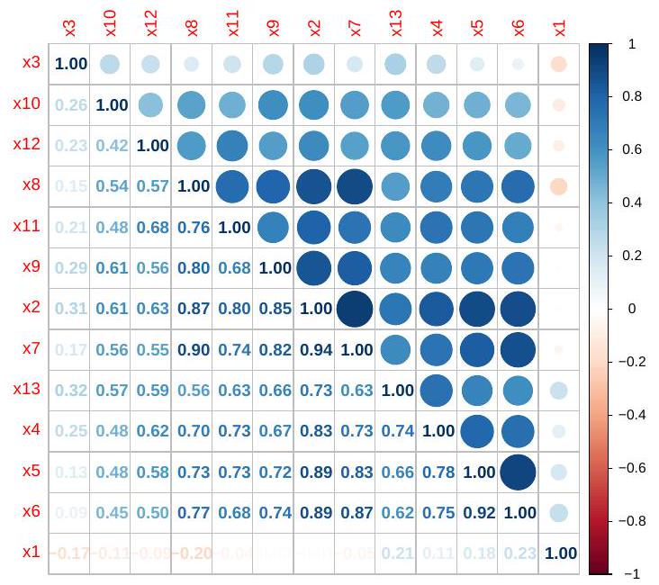
معدلات التغيير مقابل الدولار الأمريكي (x1)، مستويات الأسعار اللوغاريتمية (x2)، ومعدلات الفائدة القصيرة الأجل (x3) والطويلة الأجل (x4). بالإضافة إلى ذلك، تحتوي مجموعة البيانات على الفروقات السعرية اللوغاريتمية مقارنة بالولايات المتحدة (x5) ومعدلات الفائدة القصيرة الأجل في الولايات المتحدة (x6)، مما يسمح بإجراء فحص متعمق للديناميات المالية الدولية.
| المعاملات | BRRE | BLE | بي إم أو بي إل إي | BMTPLE | |||||||
| MLE |
|
|
|
|
|
|
|
|
|
||
| اعتراض | -3.75619 | -3.75044 | -3.34645 | -3.73475 | -3.73753 | -3.36101 | -3.20130 | -3.24421 | -2.78289 | -3.24745 | -3.24348 |
|
|
0.25804 | 0.25828 | 0.27220 | 0.25891 | 0.25880 | 0.27414 | 0.28064 | 0.27890 | 0.29769 | 0.27876 | 0.27892 |
|
|
0.17325 | 0.17224 | 0.10060 | 0.16950 | 0.16999 | 0.10425 | 0.07637 | 0.08386 | 0.00331 | 0.08442 | 0.08373 |
|
|
-0.03786 | -0.02717 | 0.49916 | 0.00141 | -0.00369 | 0.68604 | 0.97860 | 0.90001 | 1.74507 | 0.89408 | 0.90134 |
|
|
2.13191 | ٢.١١٩٦٣ | 1.51439 | 2.08689 | ٢.٠٩٢٧٣ | 1.30198 | 0.96657 | 1.05667 | 0.08783 | 1.06347 | 1.05514 |
|
|
-0.42388 | -0.42320 | -0.36898 | -0.42133 | -0.42166 | -0.37694 | -0.35797 | -0.36307 | -0.30827 | -0.36345 | -0.36298 |
|
|
٥.٠٣٧٦٧ | 5.02138 | ٣.٨٨٥٦٤ | ٤.٩٧٦٨٩ | ٤.٩٨٤٧٨ | 3.91712 | ٣.٤٦٤٢٦ | ٣.٥٨٥٩٢ | ٢.٢٧٧٨٢ | ٣.٥٩٥١٠ | ٣.٥٨٣٨٦ |
| MSE | ٣٥.١٤٥٢٥ | ٣٤.٦٥٢٧٦ | 17.09468 | ٣٣.٣٦٢٣٨ | ٣٣.٥٨٩٥٩ | 14.04834 | 12.58487 | 12.57863 | ٢٨.٠٢٩٢٢ | 12.59006 | 12.57629 |
6. الخاتمة
تتأكد الفائدة العملية لمقدّر ليو المعدل من خلال تطبيقين تجريبيين، حيث أنتج باستمرار قيم MSE أقل مقارنةً بأساليب MLE وBRRE وBLE. تشير هذه النتائج مجتمعة إلى أن مقدّر TPBR يمثل حلاً فعالاً لتحليل الانحدار الذي يتضمن متنبئين متداخلين، مما يوفر دقة تقدير محسّنة عبر كل من مجموعات البيانات المحاكية والواقعية.
مساهمات المؤلفين
بيان توفر البيانات
تعارض المصالح
References
2.Abdelwahab, M. M., Abonazel, M. R., Hammad, A. T., and El-Masry, A. M. (2024). Modified twoparameter liu estimator for addressing multicollinearity in the poisson regression model. Axioms, 13(1):46.
3.Abonazel, M. R. (2023). New modified two-parameter liu estimator for the conway-maxwell poisson regression model. Journal of Statistical Computation and Simulation, 93(12):1976-1996.
4.Abonazel, M. R. (2025). A new biased estimation class to combat the multicollinearity in regression models: Modified two-parameter liu estimator. Computational Journal of Mathematical and Statistical Sciences, 4(1):316-347.
5.Abonazel, M. R., Awwad, F. A., Tag Eldin, E., Kibria, B. M. G., and Khattab, I. G. (2023). Developing a two-parameter liu estimator for the com-poisson regression model: Application and simulation. Frontiers in Applied Mathematics and Statistics, 9:956963.
6.Abonazel, M. R. and Taha, I. M. (2023). Beta ridge regression estimators: simulation and application. Communications in Statistics-Simulation and Computation, 52(9):4280-4292.
7.Akhtar, N. and Alharthi, M. F. (2024). A comparative study of the performance of new ridge estimators for multicollinearity: Insights from simulation and real data application. AIP Advances, 14(11).
8.Algamal, Z. Y. (2019). A particle swarm optimization method for variable selection in beta regression model. Electronic Journal of Applied Statistical Analysis, 12(2).
9.Algamal, Z. Y. and Abonazel, M. R. (2022). Developing a liu-type estimator in beta regression model. Concurrency and Computation: Practice and Experience, 34(5):e6685.
10.Allenbrand, C. and Sherwood, B. (2023). Model selection uncertainty and stability in beta regression models: A study of bootstrap-based model averaging with an empirical application to clickstream data. The Annals of Applied Statistics, 17(1):680-710.
11.Amin, M., Akram, M. N., and Kibria, B. M. G. (2021). A new adjusted liu estimator for the poisson regression model. Concurrency and computation: Practice and experience, 33(20):e6340.
12.Amin, M., Ashraf, H., Bakouch, H. S., and Qarmalah, N. (2023). James stein estimator for the beta regression model with application to heat-treating test and body fat datasets. Axioms, 12(6):526.
13.Coakley, J., Fuertes, A., and Smith, R. (2006). Unobserved heterogeneity in panel time series models. Computational Statistics & Data Analysis, 50(9):2361-2380.
14.Dawoud, I. and Kibria, B. M. G. (2020). A new biased estimator to combat the multicollinearity of the gaussian linear regression model. Stats, 3(4):526-541.
15.Dertli, H. I., Hayes, D. B., and Zorn, T. G. (2024). Effects of multicollinearity and data granularity on regression models of stream temperature. Journal of Hydrology, 639:131572.
16.Dobson, A. J. and Barnett, A. G. (2018). An introduction to generalized linear models. Chapman and Hall/CRC.
17.Erkoç, A., Ertan, E., Algamal, Z. Y., and Akay, K. U. (2023). The beta liu-type estimator: simulation and application. Hacettepe Journal of Mathematics and Statistics, 52(3):828-840.
18.Farebrother, R. W. (1976). Further results on the mean square error of ridge regression. Journal of the Royal Statistical Society. Series B (Methodological), pages 248-250.
19.Ferrari, S. and Cribari-Neto, F. (2004). Beta regression for modelling rates and proportions. Journal of applied statistics, 31(7):799-815.
20.Frisch, R. (1997). Statistical confluence analysis by means of complete regression systems (1934). The Foundations of Econometric Analysis, page 271.
21.Geissinger, E. A., Khoo, C. L. L., Richmond, I. C., Faulkner, S. J. M., and Schneider, D. C. (2022). A case for beta regression in the natural sciences. Ecosphere, 13(2):e3940.
22.Hoerl, A. E. and Kennard, R. W. (1970). Ridge regression: Biased estimation for nonorthogonal problems. Technometrics, 12(1):55-67.
23. Karlsson, P., Månsson, K., and Kibria, B. M. G. (2020). A liu estimator for the beta regression model and its application to chemical data. Journal of Chemometrics, 34(10):e3300.
24.Khan, M. S., Ali, A., Suhail, M., Awwad, F. A., Ismail, E. A. A., and Ahmad, H. (2023). On the performance of two-parameter ridge estimators for handling multicollinearity problem in linear regression: Simulation and application. AIP Advances, 13(11).
25.Kibria, B. M. G. and Lukman, A. F. et al. (2020). A new ridge-type estimator for the linear regression model: Simulations and applications. Scientifica, 2020.
26.Koç, T. and Dünder, E. (2024). Jackknife kibria-lukman estimator for the beta regression model. Communications in Statistics-Theory and Methods, 53(21):7789-7805.
27.Kyriazos, T. and Poga, M. (2023). Dealing with multicollinearity in factor analysis: the problem, detections, and solutions. Open Journal of Statistics, 13(3):404-424.
28.Liu, K. (1993). A new class of biased estimate in linear regression. Communications in Statistics-Theory and Methods, 22(2):393-402.
29.Liu, K. (2003). Using liu-type estimator to combat collinearity. Communications in Statistics-Theory and Methods, 32(5):1009-1020.
30.Lukman, A. F., Ayinde, K., Binuomote, S., and Clement, O. A. (2019). Modified ridge-type estimator to combat multicollinearity: Application to chemical data. Journal of Chemometrics, 33(5):e3125.
31.Lukman, A. F., Ayinde, K., Kibria, B. M. G., and Adewuyi, E. T. (2022). Modified ridge-type estimator for the gamma regression model. Communications in Statistics-Simulation and Computation, 51(9):50095023.
32.Lukman, A. F., Kibria, B. M. G., Ayinde, K., and Jegede, S. L. (2020). Modified one-parameter liu estimator for the linear regression model. Modelling and Simulation in Engineering, 2020:1-17.
33.Mahmood, S. W., Seyala, N. N., and Algamal, Z. Y. (2020). Adjusted r2-type measures for beta regression model. Electron J Appl Stat Anal, 13(2):350-357.
34.Özkale, M. R. and Kaciranlar, S. (2007). The restricted and unrestricted two-parameter estimators. Communications in Statistics-Theory and Methods, 36(15):2707-2725.
35.Penrose, K. W., Nelson, A. G., and Fisher, A. G. (1985). Generalized body composition prediction equation for men using simple measurement techniques. Medicine & Science in Sports E Exercise, 17(2):189.
36.Qasim, M., Månsson, K., and Kibria, B. M. G. (2021). On some beta ridge regression estimators: method, simulation and application. Journal of Statistical Computation and Simulation, 91(9):1699-1712.
37.Segerstedt, B. (1992). On ordinary ridge regression in generalized linear models. Communications in Statistics-Theory and Methods, 21(8):2227-2246.
38.Stein, C. (1956). Inadmissibility of the usual estimator for the mean of a multivariate normal distribution. Technical report, Stanford University, Stanford, CA, USA.
39.Trenkler, G. and Toutenburg, H. (1990). Mean squared error matrix comparisons between biased esti-mators-an overview of recent results. Statistical papers, 31(1):165-179.
40.Tsagris, M. and Pandis, N. (2021). Multicollinearity. American journal of orthodontics and dentofacial orthopedics, 159(5):695-696.
© 2025 by the authors. Disclaimer/Publisher’s Note: The content in all publications reflects the views, opinions, and data of the respective individual author(s) and contributor(s), and not those of Sphinx Scientific Press (SSP) or the editor(s). SSP and/or the editor(s) explicitly state that they are not liable for any harm to individuals or property arising from the ideas, methods, instructions, or products mentioned in the content.
DOI: https://doi.org/10.64389/mjs.2025.01111
Publication Date: 2025-07-12
Research article
New Modified Liu Estimators to Handle the Multicollinearity in the Beta Regression Model: Simulation and Applications
ARTICLE INFO
Keywords:
Modified Liu estimator
Multicollinearity
Biased estimators
Ridge estimator
Mathematics Subject Classification:
Important Dates:
Revised: 7 July 2025
Accepted: 10 July 2025
Online: 12 July 2025
Abstract
The beta regression model (BRM) is widely used for analyzing bounded response variables, such as proportions, percentages. However, when multicollinearity exists among explanatory variables, the conventional maximum likelihood estimator (MLE) becomes unstable and inefficient. To address this issue, we propose new modified Liu estimators for the BRM, designed to enhance estimation accuracy in the presence of high multicollinearity among predictors. The proposed estimators extend the traditional Liu estimator by incorporating flexible biasing parameters, offering a more robust alternative to the MLE. Theoretical comparisons demonstrate the superiority of the new estimators over existing methods. Additionally, Monte Carlo simulations and real-world applications evidence their improved performance in terms of mean squared error (MSE) and mean absolute error (MAE). The results indicate that the proposed estimators significantly reduce estimation bias and variance under multicollinearity, providing more reliable regression coefficients.
1. Introduction
reported that these two-parameter estimators perform better than single-parameter alternatives. Building on this foundation, the present study proposed modified Liu parameters for BRM. We propose a new modified one and two-parameter Liu estimator specifically designed to reduce the effects of multicollinearity in BRM. We present systematic methods for selecting the optimal parameters and conduct detailed performance comparisons using simulation and applications with existing methods, including MLE, ridge, and Liu estimators.
2. Methodology
To address multicollinearity challenges in BRM, Karlsson et al. [23] proposed the Beta Liu Estimator (BLE), demonstrating superior performance compared to traditional BRRE. The BLE is formally defined as:
- At
, the BLE simplifies to the MLE. - For
, the BLE produces shrunken coefficients, effectively mitigating multicollinearity effects.
3. Proposed Estimators
3.1. Beta modified one-parameter Liu estimator
3.2. Beta modified two-parameter Liu estimator
3.3. Theoretical comparison using MMSE and scalar MSE
Lemma 1. For any positive definite matrix
Proof:
Theorem 2. MMSE
Proof:
Theorem 3. MMSE
Proof:
Theorem 4.
Proof:
3.4. Selection of biasing parameter
4. Monte Carlo Simulation
|
|
n | BRRE | BLE | BMOPLE | BMTPLE | |||||||
| MLE |
|
|
|
|
|
|
|
|
|
|||
| 0.80 | 30 | 0.59865 | 0.54371 | 0.49854 | 0.56211 | 0.39102 | 0.39102 | 0.37994 | 0.33192 | 0.20262 | 0.34711 | 0.28845 |
| 75 | 0.19933 | 0.19256 | 0.18632 | 0.19933 | 0.17260 | 0.17260 | 0.16869 | 0.15986 | 0.09519 | 0.16513 | 0.15060 | |
| 150 | 0.11661 | 0.11402 | 0.11265 | 0.11661 | 0.10658 | 0.10658 | 0.10331 | 0.09981 | 0.08418 | 0.10228 | 0.09610 | |
| 200 | 0.11329 | 0.11116 | 0.10977 | 0.11329 | 0.10491 | 0.10491 | 0.10251 | 0.09944 | 0.07102 | 0.10162 | 0.09612 | |
| 300 | 0.09902 | 0.09755 | 0.09668 | 0.09902 | 0.09322 | 0.09322 | 0.09092 | 0.08876 | 0.06318 | 0.09028 | 0.08641 | |
| 400 | 0.06504 | 0.06430 | 0.06370 | 0.06504 | 0.06210 | 0.06210 | 0.06054 | 0.05951 | 0.05806 | 0.06027 | 0.05837 | |
| 0.85 | 30 | 0.84338 | 0.76349 | 0.71370 | 0.73158 | 0.52125 | 0.52125 | 0.49182 | 0.42789 | 0.24850 | 0.43504 | 0.36954 |
| 75 | 0.30541 | 0.29075 | 0.27662 | 0.30094 | 0.24410 | 0.24410 | 0.23899 | 0.22051 | 0.13431 | 0.23153 | 0.20178 | |
| 150 | 0.20878 | 0.20105 | 0.19498 | 0.20878 | 0.17764 | 0.17764 | 0.17393 | 0.16354 | 0.09076 | 0.17027 | 0.15263 | |
| 200 | 0.12849 | 0.12535 | 0.12227 | 0.12849 | 0.11648 | 0.11648 | 0.11359 | 0.10901 | 0.06146 | 0.11215 | 0.10409 | |
| 300 | 0.11050 | 0.10836 | 0.10621 | 0.11050 | 0.10211 | 0.10211 | 0.09953 | 0.09637 | 0.05833 | 0.09861 | 0.09294 | |
| 400 | 0.10401 | 0.10245 | 0.10122 | 0.10401 | 0.09716 | 0.09716 | 0.09518 | 0.09275 | 0.06649 | 0.09466 | 0.09009 | |
| 0.90 | 30 | 0.97613 | 0.85885 | 0.74545 | 0.71295 | 0.50368 | 0.50368 | 0.48818 | 0.40588 | 0.42283 | 0.42927 | 0.33484 |
| 75 | 0.44011 | 0.40812 | 0.37435 | 0.42929 | 0.30917 | 0.30917 | 0.30259 | 0.26617 | 0.17612 | 0.28607 | 0.23098 | |
| 150 | 0.25209 | 0.24082 | 0.23379 | 0.25209 | 0.20571 | 0.20571 | 0.20091 | 0.18573 | 0.10259 | 0.19494 | 0.17021 | |
| 200 | 0.15451 | 0.14963 | 0.14485 | 0.15451 | 0.13449 | 0.13449 | 0.13113 | 0.12405 | 0.04949 | 0.12798 | 0.11656 | |
| 300 | 0.17619 | 0.17159 | 0.16822 | 0.17619 | 0.15751 | 0.15751 | 0.15411 | 0.14728 | 0.08178 | 0.15207 | 0.13996 | |
| 400 | 0.12033 | 0.11756 | 0.11509 | 0.12033 | 0.10948 | 0.10948 | 0.10656 | 0.10225 | 0.05919 | 0.10534 | 0.09764 | |
| 0.95 | 30 | 1.95145 | 1.61153 | 1.33847 | 0.74971 | 0.63125 | 0.63125 | 0.60304 | 0.46309 | 0.75117 | 0.46704 | 0.36082 |
| 75 | 0.77058 | 0.68403 | 0.59467 | 0.67190 | 0.40887 | 0.40887 | 0.39664 | 0.32293 | 0.29066 | 0.34976 | 0.25791 | |
| 150 | 0.65448 | 0.61273 | 0.57333 | 0.46494 | 0.40631 | 0.40631 | 0.39867 | 0.35792 | 0.26362 | 0.37198 | 0.31806 | |
| 200 | 0.46969 | 0.44678 | 0.43155 | 0.39893 | 0.33836 | 0.33836 | 0.33232 | 0.30280 | 0.20512 | 0.31955 | 0.27328 | |
| 300 | 0.30380 | 0.28634 | 0.26932 | 0.30325 | 0.23318 | 0.23318 | 0.22857 | 0.20623 | 0.09539 | 0.21881 | 0.18363 | |
| 400 | 0.24916 | 0.23768 | 0.22492 | 0.24784 | 0.20084 | 0.20084 | 0.19702 | 0.18129 | 0.09088 | 0.19109 | 0.16502 | |
| 0.99 | 30 | 14.14444 | 10.76913 | 9.79942 | 1.91565 | 0.41671 | 0.41671 | 0.38925 | 0.27750 | 2.31218 | 0.16890 | 0.22069 |
| 75 | 3.78885 | 3.02737 | 2.62939 | 0.37407 | 0.53995 | 0.53995 | 0.50980 | 0.34694 | 1.03086 | 0.26050 | 0.24739 | |
| 150 | 2.29274 | 1.84316 | 1.52954 | 0.57198 | 0.48478 | 0.48478 | 0.45777 | 0.30119 | 0.79692 | 0.29312 | 0.19747 | |
| 200 | 1.70053 | 1.41316 | 1.18927 | 0.70098 | 0.49920 | 0.49920 | 0.47538 | 0.33489 | 0.64845 | 0.35025 | 0.23149 | |
| 300 | 1.34593 | 1.15361 | 0.98523 | 0.75240 | 0.48773 | 0.48773 | 0.46838 | 0.34919 | 0.63455 | 0.38140 | 0.25647 | |
| 400 | 1.06164 | 0.90709 | 0.76542 | 0.74014 | 0.42958 | 0.42958 | 0.41236 | 0.30474 | 0.42084 | 0.33755 | 0.21832 | |
|
|
n | BRRE | BLE | BMOPLE | BMTPLE | |||||||
| MLE |
|
|
|
|
|
|
|
|
|
|||
| 0.80 | 30 | 0.64750 | 0.52111 | 0.42427 | 0.45862 | 0.45128 | 0.40733 | 0.41213 | 0.38837 | 0.16780 | 0.38943 | 0.35503 |
| 75 | 0.15702 | 0.14471 | 0.13449 | 0.15652 | 0.14051 | 0.13388 | 0.12976 | 0.12605 | 0.06906 | 0.12810 | 0.12061 | |
| 150 | 0.09021 | 0.08601 | 0.08350 | 0.09021 | 0.08440 | 0.08332 | 0.07876 | 0.07751 | 0.07712 | 0.07827 | 0.07564 | |
| 200 | 0.08276 | 0.07930 | 0.07664 | 0.08276 | 0.07808 | 0.07656 | 0.07295 | 0.07186 | 0.05689 | 0.07260 | 0.07017 | |
| 300 | 0.07660 | 0.07372 | 0.07153 | 0.07660 | 0.07262 | 0.07149 | 0.06802 | 0.06704 | 0.04608 | 0.06769 | 0.06554 | |
| 400 | 0.04074 | 0.03973 | 0.03887 | 0.04074 | 0.03938 | 0.03885 | 0.03680 | 0.03649 | 0.04957 | 0.03668 | 0.03601 | |
| 0.85 | 30 | 0.56840 | 0.44911 | 0.38988 | 0.42134 | 0.38533 | 0.37133 | 0.32529 | 0.30210 | 0.12344 | 0.29520 | 0.27365 |
| 75 | 0.21368 | 0.18830 | 0.16699 | 0.20885 | 0.17881 | 0.16503 | 0.16601 | 0.15803 | 0.05910 | 0.16179 | 0.14713 | |
| 150 | 0.15136 | 0.13888 | 0.12834 | 0.14881 | 0.13404 | 0.12771 | 0.12515 | 0.12109 | 0.05286 | 0.12348 | 0.11523 | |
| 200 | 0.09343 | 0.08869 | 0.08489 | 0.09343 | 0.08696 | 0.08478 | 0.08055 | 0.07892 | 0.04151 | 0.07996 | 0.07648 | |
| 300 | 0.08379 | 0.07984 | 0.07630 | 0.08379 | 0.07835 | 0.07620 | 0.07292 | 0.07153 | 0.03097 | 0.07235 | 0.06944 | |
| 400 | 0.06466 | 0.06230 | 0.06021 | 0.06466 | 0.06149 | 0.06016 | 0.05690 | 0.05612 | 0.03517 | 0.05666 | 0.05490 | |
| 0.90 | 30 | 0.83745 | 0.61988 | 0.46531 | 0.46258 | 0.48474 | 0.42572 | 0.43904 | 0.39826 | 0.17644 | 0.39233 | 0.35028 |
| 75 | 0.39174 | 0.32949 | 0.27112 | 0.33751 | 0.29292 | 0.26584 | 0.27448 | 0.25572 | 0.09356 | 0.26294 | 0.23160 | |
| 150 | 0.17707 | 0.15849 | 0.14698 | 0.17696 | 0.15092 | 0.14570 | 0.13695 | 0.13083 | 0.04159 | 0.13374 | 0.12243 | |
| 200 | 0.12556 | 0.11622 | 0.10920 | 0.12541 | 0.11262 | 0.10893 | 0.10354 | 0.10031 | 0.03265 | 0.10212 | 0.09563 | |
| 300 | 0.09785 | 0.09181 | 0.08699 | 0.09785 | 0.08955 | 0.08680 | 0.08262 | 0.08047 | 0.02875 | 0.08167 | 0.07733 | |
| 400 | 0.08634 | 0.08165 | 0.07753 | 0.08634 | 0.07989 | 0.07738 | 0.07356 | 0.07187 | 0.02584 | 0.07289 | 0.06935 | |
| 0.95 | 30 | 1.68443 | 1.09561 | 0.77204 | 0.48652 | 0.68062 | 0.62751 | 0.57881 | 0.50033 | 0.32582 | 0.44611 | 0.42852 |
| 75 | 0.73111 | 0.54663 | 0.39375 | 0.47995 | 0.43239 | 0.36634 | 0.39682 | 0.35168 | 0.12190 | 0.35665 | 0.30196 | |
| 150 | 0.37054 | 0.30386 | 0.24197 | 0.31657 | 0.26622 | 0.23681 | 0.24696 | 0.22742 | 0.07983 | 0.23379 | 0.20314 | |
| 200 | 0.27551 | 0.23754 | 0.21064 | 0.26342 | 0.21795 | 0.20874 | 0.19910 | 0.18651 | 0.05127 | 0.19220 | 0.17011 | |
| 300 | 0.25655 | 0.22332 | 0.19001 | 0.24689 | 0.20769 | 0.18726 | 0.19444 | 0.18341 | 0.04651 | 0.18890 | 0.16850 | |
| 400 | 0.18348 | 0.16438 | 0.14629 | 0.17802 | 0.15497 | 0.14527 | 0.14403 | 0.13731 | 0.03603 | 0.14085 | 0.12803 | |
| 0.99 | 30 | 6.93854 | 2.90235 | 2.26384 | 0.86870 | 0.32289 | 0.31842 | 0.21776 | 0.15566 | 0.44098 | 0.16182 | 0.13505 |
| 75 | 2.91424 | 1.59392 | 1.11270 | 0.18493 | 0.51965 | 0.49462 | 0.41557 | 0.30699 | 0.41887 | 0.19873 | 0.24476 | |
| 150 | 2.16375 | 1.39194 | 1.02453 | 0.29387 | 0.57347 | 0.52891 | 0.48072 | 0.37903 | 0.35615 | 0.30998 | 0.30361 | |
| 200 | 1.52260 | 1.01553 | 0.71168 | 0.39518 | 0.54538 | 0.49432 | 0.47786 | 0.39059 | 0.31249 | 0.36324 | 0.31620 | |
| 300 | 1.28047 | 0.88479 | 0.59777 | 0.48224 | 0.54690 | 0.48200 | 0.48736 | 0.40500 | 0.25899 | 0.39680 | 0.33012 | |
| 400 | 0.98168 | 0.69490 | 0.48538 | 0.47849 | 0.47422 | 0.41223 | 0.42778 | 0.36201 | 0.18815 | 0.36141 | 0.29878 | |
The
5. Applications
|
|
n | BRRE | BLE | BMTPLE | ||||||||
| MLE |
|
|
|
|
BMOPLE |
|
|
|
|
|
||
| 0.80 | 30 | 2.64169 | 2.40458 | 2.10650 | 1.77960 | 1.33606 | 1.33567 | 1.29169 | 1.14548 | 0.45200 | 0.99216 | 0.80629 |
| 75 | 1.10480 | 1.07215 | 1.04870 | 0.65330 | 0.64745 | 0.64745 | 0.60047 | 0.56443 | 0.16792 | 0.51434 | 0.46595 | |
| 150 | 0.47603 | 0.46338 | 0.45160 | 0.46713 | 0.41723 | 0.41720 | 0.39379 | 0.37521 | 0.11558 | 0.37783 | 0.32299 | |
| 200 | 0.33721 | 0.33028 | 0.32274 | 0.33721 | 0.30710 | 0.30710 | 0.28923 | 0.27844 | 0.07285 | 0.28030 | 0.24701 | |
| 300 | 0.31110 | 0.30516 | 0.30200 | 0.28159 | 0.27915 | 0.27915 | 0.25681 | 0.24986 | 0.08806 | 0.24978 | 0.22903 | |
| 400 | 0.28495 | 0.28147 | 0.27930 | 0.28080 | 0.26548 | 0.26548 | 0.25224 | 0.24652 | 0.08035 | 0.24759 | 0.22935 | |
| 0.85 | 30 | 2.87692 | 2.63193 | 2.33615 | 1.87831 | 1.31017 | 1.30979 | 1.24291 | 1.08697 | 0.40597 | 0.92900 | 0.73996 |
| 75 | 1.08265 | 1.03854 | 0.99123 | 0.91909 | 0.78523 | 0.78523 | 0.75382 | 0.70133 | 0.14955 | 0.67579 | 0.56095 | |
| 150 | 0.53274 | 0.51535 | 0.50001 | 0.53274 | 0.45060 | 0.45060 | 0.42550 | 0.40029 | 0.10548 | 0.40236 | 0.33068 | |
| 200 | 0.39951 | 0.38841 | 0.37884 | 0.39951 | 0.35090 | 0.35090 | 0.32722 | 0.31093 | 0.06772 | 0.31213 | 0.26458 | |
| 300 | 0.44089 | 0.43337 | 0.42737 | 0.39901 | 0.38634 | 0.38634 | 0.36734 | 0.35644 | 0.09867 | 0.35664 | 0.32423 | |
| 400 | 0.24624 | 0.24185 | 0.23885 | 0.24624 | 0.22792 | 0.22792 | 0.21241 | 0.20523 | 0.04804 | 0.20649 | 0.18411 | |
| 0.90 | 30 | 4.48462 | 3.90853 | 3.34183 | 1.76829 | 1.52439 | 1.52439 | 1.48083 | 1.25481 | 0.83019 | 0.89733 | 0.82254 |
| 75 | 1.57276 | 1.47943 | 1.32581 | 1.50402 | 1.06089 | 1.06089 | 1.02829 | 0.92375 | 0.28273 | 0.89047 | 0.66320 | |
| 150 | 0.76350 | 0.72929 | 0.69584 | 0.76350 | 0.59480 | 0.59480 | 0.56200 | 0.51623 | 0.10481 | 0.51124 | 0.39543 | |
| 200 | 0.66836 | 0.64669 | 0.62930 | 0.61539 | 0.54225 | 0.54225 | 0.50468 | 0.47474 | 0.08066 | 0.46773 | 0.39156 | |
| 300 | 0.65632 | 0.64172 | 0.62826 | 0.59069 | 0.54129 | 0.54129 | 0.51659 | 0.49443 | 0.13431 | 0.49182 | 0.43091 | |
| 400 | 0.40050 | 0.39055 | 0.38242 | 0.40050 | 0.35514 | 0.35514 | 0.33309 | 0.31729 | 0.05772 | 0.31926 | 0.27206 | |
| 0.95 | 30 | 8.66006 | 7.30329 | 6.04024 | 1.49363 | 1.63259 | 1.63259 | 1.59365 | 1.31432 | 0.98935 | 0.56670 | 0.81276 |
| 75 | 2.43238 | 2.22344 | 1.93829 | 2.07747 | 1.24529 | 1.24529 | 1.21509 | 1.04092 | 0.39006 | 0.90334 | 0.65857 | |
| 150 | 1.79797 | 1.66360 | 1.47969 | 1.71622 | 1.06254 | 1.06254 | 1.03175 | 0.89822 | 0.29090 | 0.82312 | 0.58913 | |
| 200 | 1.26987 | 1.19753 | 1.09461 | 1.24894 | 0.88111 | 0.88111 | 0.84936 | 0.76029 | 0.15425 | 0.73623 | 0.53766 | |
| 300 | 0.87923 | 0.83916 | 0.79237 | 0.86756 | 0.66557 | 0.66557 | 0.63796 | 0.58192 | 0.11254 | 0.57548 | 0.43693 | |
| 400 | 2.40333 | 2.34172 | 2.30651 | 1.08319 | 0.98300 | 0.98300 | 0.91888 | 0.86690 | 0.11773 | 0.75832 | 0.72395 | |
| 0.99 | 30 | 46.53267 | 39.13653 | 33.84793 | 4.56365 | 1.02191 | 1.02191 | 1.00490 | 0.82855 | 3.30725 | 2.53352 | 0.53972 |
| 75 | 14.31168 | 12.59060 | 10.78966 | 1.09636 | 1.51731 | 1.51731 | 1.49352 | 1.19007 | 1.50903 | 0.26156 | 0.65130 | |
| 150 | 8.56375 | 7.60768 | 6.50498 | 1.79189 | 1.48829 | 1.48829 | 1.46132 | 1.15434 | 1.17424 | 0.45137 | 0.61263 | |
| 200 | 5.91519 | 5.27114 | 4.47002 | 2.37686 | 1.52570 | 1.52570 | 1.50343 | 1.19409 | 0.65663 | 0.65281 | 0.60015 | |
| 300 | 4.52595 | 4.08005 | 3.41682 | 2.63069 | 1.53344 | 1.53327 | 1.58315 | 1.23394 | 0.75394 | 0.87444 | 0.67794 | |
| 400 | 5.78554 | 5.40341 | 4.89124 | 2.76026 | 1.70205 | 1.70205 | 1.67444 | 1.41825 | 0.64502 | 0.98075 | 0.88845 | |
|
|
n | BRRE | BLE | BMTPLE | ||||||||
| MLE |
|
|
|
|
BMOPLE |
|
|
|
|
|
||
| 0.80 | 30 | 1.83877 | 1.44699 | 1.06422 | 1.18693 | 1.14327 | 0.97437 | 1.01112 | 0.92170 | 0.30634 | 0.77951 | 0.71436 |
| 75 | 0.57997 | 0.53073 | 0.47991 | 0.54481 | 0.49251 | 0.46933 | 0.44340 | 0.42461 | 0.09565 | 0.41621 | 0.36792 | |
| 150 | 0.30259 | 0.28380 | 0.26640 | 0.30167 | 0.27454 | 0.26559 | 0.24252 | 0.23418 | 0.06719 | 0.23253 | 0.20836 | |
| 200 | 0.22476 | 0.21404 | 0.20312 | 0.22476 | 0.20937 | 0.20280 | 0.18487 | 0.18010 | 0.05297 | 0.17933 | 0.16465 | |
| 300 | 0.21275 | 0.20346 | 0.19590 | 0.21275 | 0.19948 | 0.19574 | 0.17411 | 0.16995 | 0.04857 | 0.16944 | 0.15625 | |
| 400 | 0.14582 | 0.14092 | 0.13678 | 0.14582 | 0.13892 | 0.13671 | 0.12238 | 0.12012 | 0.04721 | 0.12006 | 0.11256 | |
| 0.85 | 30 | 1.82500 | 1.45547 | 1.07658 | 1.18792 | 1.12901 | 1.00693 | 1.01537 | 0.92390 | 0.29687 | 0.78769 | 0.71469 |
| 75 | 0.65561 | 0.58562 | 0.51427 | 0.64153 | 0.53991 | 0.50876 | 0.47695 | 0.45069 | 0.08164 | 0.43515 | 0.37568 | |
| 150 | 0.42016 | 0.38795 | 0.35740 | 0.41946 | 0.37053 | 0.35598 | 0.32902 | 0.31539 | 0.07141 | 0.31158 | 0.27418 | |
| 200 | 0.37313 | 0.34939 | 0.32569 | 0.36966 | 0.33489 | 0.32380 | 0.29477 | 0.28452 | 0.04316 | 0.28121 | 0.25220 | |
| 300 | 0.23383 | 0.22290 | 0.21314 | 0.23383 | 0.21750 | 0.21286 | 0.19323 | 0.18803 | 0.04010 | 0.18735 | 0.17127 | |
| 400 | 0.21292 | 0.20401 | 0.19618 | 0.21292 | 0.19981 | 0.19603 | 0.17672 | 0.17250 | 0.03321 | 0.17197 | 0.15862 | |
| 0.90 | 30 | 4.26488 | 3.02389 | 2.07686 | 1.13010 | 1.65646 | 1.52159 | 1.42122 | 1.27032 | 0.71327 | 0.84827 | 0.97675 |
| 75 | 0.96233 | 0.82457 | 0.64968 | 0.85692 | 0.70945 | 0.62838 | 0.64029 | 0.58953 | 0.13196 | 0.55113 | 0.46057 | |
| 150 | 0.68256 | 0.61024 | 0.53307 | 0.67437 | 0.56186 | 0.52849 | 0.50150 | 0.47141 | 0.07558 | 0.45728 | 0.38752 | |
| 200 | 0.48817 | 0.45086 | 0.41836 | 0.45866 | 0.41998 | 0.40534 | 0.37401 | 0.35828 | 0.04965 | 0.35098 | 0.31104 | |
| 300 | 0.33067 | 0.30821 | 0.28691 | 0.33067 | 0.29656 | 0.28614 | 0.26091 | 0.25065 | 0.03357 | 0.24815 | 0.21923 | |
| 400 | 0.32034 | 0.30122 | 0.28391 | 0.32034 | 0.28935 | 0.28271 | 0.25730 | 0.24801 | 0.03325 | 0.24654 | 0.21915 | |
| 0.95 | 30 | 7.49130 | 5.17984 | 3.59262 | 0.82873 | 1.99582 | 1.93539 | 1.71198 | 1.50775 | 0.71993 | 0.63689 | 1.14818 |
| 75 | 1.85635 | 1.47272 | 1.06156 | 1.24485 | 1.05443 | 0.96045 | 0.96265 | 0.85110 | 0.19345 | 0.69663 | 0.61571 | |
| 150 | 1.52308 | 1.26653 | 0.97146 | 1.18191 | 0.98375 | 0.89465 | 0.89512 | 0.80985 | 0.15599 | 0.70891 | 0.60865 | |
| 200 | 1.15016 | 1.01552 | 0.84704 | 0.93563 | 0.82545 | 0.75061 | 0.75308 | 0.70096 | 0.09803 | 0.65054 | 0.56469 | |
| 300 | 0.76535 | 0.67981 | 0.57337 | 0.75647 | 0.61234 | 0.56729 | 0.55279 | 0.51534 | 0.05813 | 0.49717 | 0.41425 | |
| 400 | 0.59861 | 0.53845 | 0.47632 | 0.59506 | 0.49941 | 0.47339 | 0.44629 | 0.42078 | 0.04042 | 0.40916 | 0.34876 | |
| 0.99 | 30 | 34.72324 | 22.88346 | 16.87703 | 7.82112 | 1.20571 | 1.20513 | 1.11674 | 0.95281 | 1.61605 | 2.77552 | 0.74712 |
| 75 | 10.10960 | 6.90541 | 4.55026 | 0.43189 | 1.59396 | 1.58933 | 1.44447 | 1.18678 | 0.72038 | 0.21227 | 0.80404 | |
| 150 | 5.68694 | 3.97307 | 2.61869 | 0.85581 | 1.38724 | 1.35887 | 1.26837 | 1.02548 | 0.47350 | 0.33012 | 0.66594 | |
| 200 | 5.18955 | 3.97351 | 2.78364 | 1.22267 | 1.64480 | 1.59475 | 1.51056 | 1.27291 | 0.33539 | 0.61082 | 0.86192 | |
| 300 | 5.04496 | 4.19987 | 3.30905 | 1.48063 | 1.82360 | 1.74464 | 1.71323 | 1.50816 | 0.32844 | 0.92600 | 1.11495 | |
| 400 | 3.00386 | 2.30031 | 1.54180 | 1.42011 | 1.31878 | 1.24651 | 1.21399 | 1.03222 | 0.25264 | 0.70063 | 0.68973 | |
5.1. Body fat dataset
|
|
n | BRRE | BLE | BMOPLE | BMTPLE | |||||||
| MLE |
|
|
|
|
|
|
|
|
|
|||
| 0.80 | 30 | 1.26890 | 1.21011 | 1.16031 | 1.20732 | 1.03130 | 1.03130 | 1.01514 | 0.95288 | 0.76332 | 0.97479 | 0.89002 |
| 75 | 0.77041 | 0.75887 | 0.74864 | 0.75442 | 0.71742 | 0.71742 | 0.70911 | 0.69288 | 0.49775 | 0.70035 | 0.67491 | |
| 150 | 0.56644 | 0.56054 | 0.55783 | 0.56644 | 0.54263 | 0.54263 | 0.53418 | 0.52629 | 0.47117 | 0.53091 | 0.51789 | |
| 200 | 0.52310 | 0.51826 | 0.51524 | 0.52310 | 0.50332 | 0.50332 | 0.49575 | 0.48843 | 0.41674 | 0.49314 | 0.48034 | |
| 300 | 0.43000 | 0.42691 | 0.42524 | 0.43000 | 0.41782 | 0.41782 | 0.41142 | 0.40756 | 0.40672 | 0.41009 | 0.40343 | |
| 400 | 0.38469 | 0.38281 | 0.38136 | 0.38469 | 0.37719 | 0.37719 | 0.37225 | 0.36990 | 0.38241 | 0.37145 | 0.36739 | |
| 0.85 | 30 | 1.30810 | 1.24576 | 1.20842 | 1.24582 | 1.04219 | 1.04219 | 1.00798 | 0.93671 | 0.71812 | 0.95073 | 0.86658 |
| 75 | 0.83302 | 0.81311 | 0.79574 | 0.83276 | 0.75189 | 0.75189 | 0.74226 | 0.71360 | 0.50549 | 0.72905 | 0.68296 | |
| 150 | 0.68893 | 0.67727 | 0.66926 | 0.68264 | 0.63840 | 0.63840 | 0.63076 | 0.61395 | 0.48316 | 0.62444 | 0.59557 | |
| 200 | 0.54907 | 0.54235 | 0.53621 | 0.54907 | 0.52213 | 0.52213 | 0.51180 | 0.50194 | 0.35977 | 0.50785 | 0.49111 | |
| 300 | 0.55313 | 0.54809 | 0.54369 | 0.54569 | 0.52959 | 0.52959 | 0.52149 | 0.51393 | 0.38609 | 0.51844 | 0.50570 | |
| 400 | 0.42353 | 0.42048 | 0.41842 | 0.42353 | 0.41147 | 0.41147 | 0.40400 | 0.39959 | 0.35302 | 0.40234 | 0.39473 | |
| 0.90 | 30 | 1.50798 | 1.41596 | 1.32717 | 1.38089 | 1.13144 | 1.13144 | 1.11369 | 1.01769 | 0.90307 | 1.04158 | 0.92667 |
| 75 | 1.07544 | 1.03594 | 0.99610 | 1.05919 | 0.90533 | 0.90533 | 0.89427 | 0.84024 | 0.58383 | 0.86522 | 0.78462 | |
| 150 | 0.73651 | 0.72044 | 0.71134 | 0.73478 | 0.67191 | 0.67191 | 0.65957 | 0.63608 | 0.45720 | 0.64867 | 0.61132 | |
| 200 | 0.64727 | 0.63728 | 0.62742 | 0.64727 | 0.60640 | 0.60640 | 0.59650 | 0.58102 | 0.41143 | 0.59072 | 0.56409 | |
| 300 | 0.57866 | 0.57122 | 0.56644 | 0.57866 | 0.54915 | 0.54915 | 0.53948 | 0.52791 | 0.36816 | 0.53474 | 0.51542 | |
| 400 | 0.48391 | 0.47819 | 0.47374 | 0.48391 | 0.46099 | 0.46099 | 0.45213 | 0.44319 | 0.32209 | 0.44841 | 0.43341 | |
| 0.95 | 30 | 2.21446 | 2.01660 | 1.86012 | 1.45822 | 1.30063 | 1.30063 | 1.27175 | 1.10764 | 1.26915 | 1.10171 | 0.96908 |
| 75 | 1.35220 | 1.27356 | 1.19147 | 1.27807 | 1.01037 | 1.01037 | 0.99433 | 0.89924 | 0.76877 | 0.93379 | 0.80541 | |
| 150 | 1.04495 | 1.00075 | 0.95115 | 1.02642 | 0.85214 | 0.85214 | 0.84115 | 0.77941 | 0.55689 | 0.80644 | 0.71580 | |
| 200 | 0.92189 | 0.89427 | 0.87577 | 0.91667 | 0.80368 | 0.80368 | 0.79104 | 0.75017 | 0.48922 | 0.77079 | 0.70707 | |
| 300 | 0.85298 | 0.83027 | 0.80871 | 0.84762 | 0.75570 | 0.75570 | 0.74545 | 0.71122 | 0.49074 | 0.72970 | 0.67501 | |
| 400 | 0.79826 | 0.78059 | 0.76236 | 0.79611 | 0.72201 | 0.72201 | 0.71300 | 0.68549 | 0.42665 | 0.70069 | 0.65556 | |
| 0.99 | 30 | 4.98237 | 4.02670 | 3.65209 | 1.20783 | 0.95493 | 0.95493 | 0.90750 | 0.70453 | 1.96597 | 0.65548 | 0.62437 |
| 75 | 2.66201 | 2.29381 | 2.06339 | 0.97448 | 1.04133 | 1.04133 | 1.00287 | 0.76464 | 1.32552 | 0.67422 | 0.60921 | |
| 150 | 2.16989 | 1.91179 | 1.70775 | 1.22874 | 1.04703 | 1.04703 | 1.01357 | 0.79476 | 1.19352 | 0.79766 | 0.62365 | |
| 200 | 2.00388 | 1.81862 | 1.65616 | 1.37323 | 1.12428 | 1.12428 | 1.09644 | 0.90877 | 1.10854 | 0.92943 | 0.74470 | |
| 300 | 1.76347 | 1.61660 | 1.47441 | 1.39948 | 1.08422 | 1.08422 | 1.06010 | 0.89471 | 0.99288 | 0.93438 | 0.74544 | |
| 400 | 1.43292 | 1.32006 | 1.20648 | 1.26329 | 0.94104 | 0.94104 | 0.92157 | 0.78702 | 0.87413 | 0.83422 | 0.66296 | |
|
|
n | BRRE | BLE | BMOPLE | BMTPLE | |||||||
| MLE |
|
|
|
|
|
|
|
|
|
|||
| 0.80 | 30 | 1.20102 | 1.07942 | 0.98547 | 1.08296 | 1.02293 | 0.96531 | 0.97588 | 0.94226 | 0.62152 | 0.94757 | 0.89928 |
| 75 | 0.62847 | 0.60414 | 0.58393 | 0.62730 | 0.59557 | 0.58287 | 0.57232 | 0.56453 | 0.37666 | 0.56788 | 0.55293 | |
| 150 | 0.51808 | 0.50642 | 0.49982 | 0.51759 | 0.50141 | 0.49922 | 0.48011 | 0.47635 | 0.42131 | 0.47791 | 0.47063 | |
| 200 | 0.43898 | 0.43010 | 0.42358 | 0.43898 | 0.42707 | 0.42339 | 0.40950 | 0.40650 | 0.35109 | 0.40813 | 0.40193 | |
| 300 | 0.40067 | 0.39413 | 0.38952 | 0.40067 | 0.39183 | 0.38941 | 0.37596 | 0.37389 | 0.34327 | 0.37495 | 0.37065 | |
| 400 | 0.35227 | 0.34725 | 0.34287 | 0.35227 | 0.34530 | 0.34281 | 0.33175 | 0.33033 | 0.34379 | 0.33117 | 0.32812 | |
| 0.85 | 30 | 1.29082 | 1.14369 | 1.06572 | 1.12278 | 1.06996 | 1.04902 | 0.97668 | 0.94023 | 0.61021 | 0.93130 | 0.89322 |
| 75 | 0.77078 | 0.72884 | 0.68939 | 0.75566 | 0.71008 | 0.68611 | 0.68414 | 0.66958 | 0.41418 | 0.67628 | 0.64902 | |
| 150 | 0.59981 | 0.57739 | 0.55954 | 0.59750 | 0.56842 | 0.55842 | 0.54543 | 0.53721 | 0.35768 | 0.54114 | 0.52513 | |
| 200 | 0.47472 | 0.46222 | 0.45158 | 0.47472 | 0.45728 | 0.45126 | 0.43833 | 0.43380 | 0.28064 | 0.43616 | 0.42688 | |
| 300 | 0.46021 | 0.45001 | 0.44109 | 0.46021 | 0.44611 | 0.44082 | 0.42718 | 0.42331 | 0.28716 | 0.42543 | 0.41763 | |
| 400 | 0.38468 | 0.37836 | 0.37286 | 0.38468 | 0.37614 | 0.37272 | 0.35942 | 0.35713 | 0.31092 | 0.35839 | 0.35365 | |
| 0.90 | 30 | 1.30178 | 1.10559 | 0.96340 | 1.07195 | 1.00405 | 0.92915 | 0.94412 | 0.88769 | 0.58647 | 0.88698 | 0.82756 |
| 75 | 0.96578 | 0.88232 | 0.80354 | 0.92726 | 0.84532 | 0.79315 | 0.81235 | 0.78363 | 0.41246 | 0.79397 | 0.74563 | |
| 150 | 0.63534 | 0.60321 | 0.58304 | 0.63420 | 0.58954 | 0.58125 | 0.56047 | 0.54819 | 0.31942 | 0.55370 | 0.53116 | |
| 200 | 0.60767 | 0.58567 | 0.56800 | 0.60640 | 0.57645 | 0.56731 | 0.55273 | 0.54439 | 0.30102 | 0.54871 | 0.53203 | |
| 300 | 0.47539 | 0.46180 | 0.45121 | 0.47506 | 0.45638 | 0.45070 | 0.43631 | 0.43145 | 0.26779 | 0.43399 | 0.42409 | |
| 400 | 0.47170 | 0.45928 | 0.44790 | 0.47170 | 0.45459 | 0.44747 | 0.43534 | 0.43064 | 0.23023 | 0.43299 | 0.42350 | |
| 0.95 | 30 | 1.83005 | 1.45630 | 1.23577 | 1.11463 | 1.20225 | 1.11250 | 1.10589 | 1.01648 | 0.81747 | 0.97654 | 0.94343 |
| 75 | 1.22700 | 1.06302 | 0.91647 | 1.04476 | 0.96104 | 0.88208 | 0.91804 | 0.86359 | 0.51272 | 0.87100 | 0.80155 | |
| 150 | 0.95041 | 0.86043 | 0.77576 | 0.88779 | 0.80639 | 0.76242 | 0.77515 | 0.74219 | 0.36077 | 0.75068 | 0.69980 | |
| 200 | 0.76013 | 0.70537 | 0.66685 | 0.75018 | 0.68067 | 0.66416 | 0.64638 | 0.62588 | 0.31795 | 0.63473 | 0.59833 | |
| 300 | 0.71381 | 0.66860 | 0.62383 | 0.70786 | 0.64736 | 0.61985 | 0.62263 | 0.60483 | 0.30424 | 0.61284 | 0.58049 | |
| 400 | 0.61864 | 0.58643 | 0.55712 | 0.61486 | 0.57235 | 0.55512 | 0.54826 | 0.53551 | 0.26198 | 0.54147 | 0.51749 | |
| 0.99 | 30 | 4.24659 | 2.70318 | 2.33588 | 1.38630 | 1.02027 | 1.00096 | 0.80996 | 0.69668 | 1.06858 | 0.66460 | 0.65892 |
| 75 | 2.49576 | 1.77818 | 1.42915 | 0.72584 | 1.10011 | 1.04701 | 0.96446 | 0.79525 | 0.85047 | 0.63058 | 0.70803 | |
| 150 | 1.85836 | 1.37046 | 1.05028 | 0.87711 | 1.00082 | 0.91331 | 0.90461 | 0.76735 | 0.67982 | 0.70980 | 0.67580 | |
| 200 | 1.52931 | 1.17794 | 0.91059 | 1.00260 | 0.94180 | 0.82212 | 0.86911 | 0.75558 | 0.56272 | 0.74145 | 0.66780 | |
| 300 | 1.53819 | 1.24739 | 1.00811 | 1.06542 | 1.02429 | 0.91281 | 0.96187 | 0.86691 | 0.55260 | 0.85668 | 0.77820 | |
| 400 | 1.34894 | 1.11942 | 0.91973 | 1.01351 | 0.95024 | 0.86294 | 0.89853 | 0.82166 | 0.52176 | 0.82139 | 0.74386 | |
5.2. Purchasing power parity dataset
|
|
n | BRRE | BLE | BMTPLE | ||||||||
| MLE |
|
|
|
|
BMOPLE |
|
|
|
|
|
||
| 0.80 | 30 | 3.24799 | 3.08053 | 2.85583 | 2.94721 | 2.41087 | 2.41070 | 2.35742 | 2.18861 | 1.33807 | 2.05595 | 1.76812 |
| 75 | 1.74786 | 1.71512 | 1.68389 | 1.74414 | 1.59687 | 1.59687 | 1.54989 | 1.49964 | 0.79421 | 1.49936 | 1.35277 | |
| 150 | 1.40415 | 1.38557 | 1.37019 | 1.40415 | 1.32853 | 1.32827 | 1.28713 | 1.25726 | 0.72518 | 1.26156 | 1.16980 | |
| 200 | 1.22838 | 1.21521 | 1.20215 | 1.22838 | 1.17186 | 1.17186 | 1.13117 | 1.10977 | 0.56402 | 1.11263 | 1.04520 | |
| 300 | 1.13470 | 1.12453 | 1.11817 | 1.13470 | 1.09200 | 1.09200 | 1.05431 | 1.03685 | 0.60762 | 1.04026 | 0.98387 | |
| 400 | 1.06166 | 1.05424 | 1.04908 | 1.06166 | 1.02848 | 1.02848 | 0.99503 | 0.98221 | 0.64253 | 0.98517 | 0.94380 | |
| 0.85 | 30 | 3.32003 | 3.15423 | 2.93653 | 3.01976 | 2.45603 | 2.45603 | 2.40995 | 2.24118 | 1.44773 | 2.11198 | 1.82642 |
| 75 | 1.94119 | 1.89526 | 1.84847 | 1.93804 | 1.71866 | 1.71866 | 1.67016 | 1.60078 | 0.75255 | 1.59290 | 1.40111 | |
| 150 | 1.57452 | 1.54828 | 1.52645 | 1.57118 | 1.45563 | 1.45563 | 1.40841 | 1.36681 | 0.71037 | 1.36927 | 1.24424 | |
| 200 | 1.46038 | 1.44062 | 1.42239 | 1.46002 | 1.37123 | 1.37123 | 1.32778 | 1.29490 | 0.63052 | 1.29809 | 1.19841 | |
| 300 | 1.36833 | 1.35463 | 1.34384 | 1.36639 | 1.30397 | 1.30397 | 1.26249 | 1.23829 | 0.60330 | 1.24184 | 1.16469 | |
| 400 | 1.18628 | 1.17595 | 1.16843 | 1.17376 | 1.13376 | 1.13376 | 1.09659 | 1.07906 | 0.54197 | 1.08061 | 1.02623 | |
| 0.90 | 30 | 4.95111 | 4.59819 | 4.21426 | 3.04224 | 2.77626 | 2.77626 | 2.70271 | 2.46628 | 2.03762 | 2.05710 | 1.95137 |
| 75 | 2.52443 | 2.44233 | 2.32748 | 2.46072 | 2.08021 | 2.08021 | 2.02783 | 1.91455 | 0.96594 | 1.86849 | 1.60415 | |
| 150 | 1.95810 | 1.91313 | 1.86840 | 1.95810 | 1.74215 | 1.74215 | 1.69180 | 1.61906 | 0.74618 | 1.61312 | 1.41014 | |
| 200 | 1.68183 | 1.65411 | 1.63239 | 1.63469 | 1.53720 | 1.53720 | 1.49094 | 1.44564 | 0.64937 | 1.44350 | 1.31198 | |
| 300 | 1.41144 | 1.39030 | 1.37342 | 1.41144 | 1.32072 | 1.32072 | 1.27195 | 1.23629 | 0.52391 | 1.23893 | 1.13070 | |
| 400 | 1.36814 | 1.35116 | 1.33877 | 1.34238 | 1.27888 | 1.27888 | 1.23284 | 1.20340 | 0.54546 | 1.20130 | 1.11532 | |
| 0.95 | 30 | 6.36047 | 5.86540 | 5.30170 | 2.70490 | 2.85906 | 2.85906 | 2.82608 | 2.54074 | 2.23691 | 1.72164 | 1.93672 |
| 75 | 3.47515 | 3.31046 | 3.08062 | 3.19764 | 2.48206 | 2.48206 | 2.44814 | 2.24615 | 1.33838 | 2.09381 | 1.73250 | |
| 150 | 2.83382 | 2.71866 | 2.56583 | 2.79501 | 2.20403 | 2.20403 | 2.16392 | 2.00662 | 1.06873 | 1.92546 | 1.58642 | |
| 200 | 2.33735 | 2.26664 | 2.17496 | 2.32031 | 1.95612 | 1.95612 | 1.90973 | 1.80133 | 0.82688 | 1.77198 | 1.49797 | |
| 300 | 2.15647 | 2.10565 | 2.05004 | 2.10512 | 1.86854 | 1.86854 | 1.82478 | 1.74034 | 0.79401 | 1.73157 | 1.50232 | |
| 400 | 1.93583 | 1.89494 | 1.85675 | 1.90890 | 1.72115 | 1.72115 | 1.67443 | 1.60643 | 0.63354 | 1.59843 | 1.40904 | |
| 0.99 | 30 | 29.43032 | 28.09644 | 27.15978 | 20.76124 | 15.21159 | 15.21159 | 15.19198 | 14.96431 | 19.92645 | 16.52488 | 14.55843 |
| 75 | 7.76743 | 7.19508 | 6.52711 | 2.27509 | 2.61244 | 2.61244 | 2.58896 | 2.26608 | 2.66858 | 1.09297 | 1.59797 | |
| 150 | 6.01823 | 5.59398 | 5.08032 | 2.98590 | 2.63256 | 2.63256 | 2.60522 | 2.27142 | 2.14151 | 1.40223 | 1.54772 | |
| 200 | 4.94292 | 4.62597 | 4.17033 | 3.45573 | 2.58825 | 2.58825 | 2.56371 | 2.23963 | 1.68152 | 1.67689 | 1.49666 | |
| 300 | 4.43194 | 4.18159 | 3.79855 | 3.56645 | 2.58987 | 2.58987 | 2.56759 | 2.27986 | 1.53233 | 1.89905 | 1.57876 | |
| 400 | 4.29458 | 4.07668 | 3.75254 | 3.49893 | 2.55104 | 2.55104 | 2.52948 | 2.26805 | 1.56940 | 1.94286 | 1.64311 | |
|
|
n | BRRE | BLE | BMOPLE | BMTPLE | |||||||
| MLE |
|
|
|
|
|
|
|
|
|
|||
| 0.80 | 30 | 3.06977 | 2.72208 | 2.32322 | 2.51256 | 2.44175 | 2.25480 | 2.29288 | 2.18688 | 1.26524 | 2.01780 | 1.92012 |
| 75 | 1.57188 | 1.50419 | 1.43823 | 1.54891 | 1.45953 | 1.42610 | 1.37602 | 1.34568 | 0.66671 | 1.33135 | 1.25154 | |
| 150 | 1.30434 | 1.26314 | 1.22484 | 1.29827 | 1.24182 | 1.22186 | 1.16635 | 1.14668 | 0.58363 | 1.14197 | 1.08269 | |
| 200 | 1.03715 | 1.01275 | 0.98776 | 1.03715 | 1.00252 | 0.98699 | 0.93771 | 0.92620 | 0.47825 | 0.92366 | 0.88828 | |
| 300 | 0.99708 | 0.97614 | 0.96036 | 0.99708 | 0.96754 | 0.96001 | 0.90607 | 0.89593 | 0.48873 | 0.89442 | 0.86216 | |
| 400 | 0.87160 | 0.85688 | 0.84511 | 0.87160 | 0.85074 | 0.84493 | 0.79452 | 0.78734 | 0.43387 | 0.78637 | 0.76252 | |
| 0.85 | 30 | 2.90435 | 2.56239 | 2.18665 | 2.38330 | 2.28252 | 2.12291 | 2.14391 | 2.03302 | 1.17625 | 1.86955 | 1.76835 |
| 75 | 1.73006 | 1.63230 | 1.53148 | 1.72512 | 1.57511 | 1.52278 | 1.47539 | 1.43195 | 0.62651 | 1.40889 | 1.30368 | |
| 150 | 1.39073 | 1.33514 | 1.28574 | 1.39045 | 1.30903 | 1.28313 | 1.22629 | 1.19995 | 0.60049 | 1.19266 | 1.11768 | |
| 200 | 1.24848 | 1.20602 | 1.16657 | 1.24848 | 1.18600 | 1.16512 | 1.10558 | 1.08479 | 0.45033 | 1.07969 | 1.01813 | |
| 300 | 1.08720 | 1.06112 | 1.03884 | 1.08720 | 1.04963 | 1.03814 | 0.98558 | 0.97213 | 0.45184 | 0.97010 | 0.92826 | |
| 400 | 1.00853 | 0.98690 | 0.96856 | 1.00853 | 0.97740 | 0.96817 | 0.91253 | 0.90169 | 0.38289 | 0.89992 | 0.86499 | |
| 0.90 | 30 | 4.34279 | 3.61523 | 2.96063 | 2.29236 | 2.72079 | 2.56665 | 2.49763 | 2.32644 | 1.72486 | 1.89891 | 1.99297 |
| 75 | 2.12100 | 1.96053 | 1.75115 | 2.05726 | 1.83769 | 1.72841 | 1.73237 | 1.66074 | 0.75384 | 1.60597 | 1.46614 | |
| 150 | 1.74714 | 1.65273 | 1.55347 | 1.74350 | 1.59258 | 1.54585 | 1.50225 | 1.45622 | 0.62532 | 1.43514 | 1.32198 | |
| 200 | 1.38030 | 1.32186 | 1.26899 | 1.37549 | 1.28803 | 1.26605 | 1.20208 | 1.17288 | 0.43788 | 1.16279 | 1.08291 | |
| 300 | 1.32476 | 1.27876 | 1.23515 | 1.32183 | 1.25351 | 1.23243 | 1.16974 | 1.14657 | 0.40274 | 1.13974 | 1.07289 | |
| 400 | 1.19504 | 1.15883 | 1.12855 | 1.19504 | 1.14095 | 1.12769 | 1.06501 | 1.04635 | 0.38924 | 1.04202 | 0.98588 | |
| 0.95 | 30 | 5.57959 | 4.53205 | 3.61387 | 2.10964 | 2.92063 | 2.82975 | 2.72637 | 2.50660 | 1.82752 | 1.63808 | 2.13143 |
| 75 | 2.93768 | 2.60371 | 2.20540 | 2.48384 | 2.23810 | 2.11297 | 2.12466 | 1.99064 | 0.93469 | 1.80039 | 1.68141 | |
| 150 | 2.51183 | 2.27637 | 1.97316 | 2.34234 | 2.05272 | 1.93463 | 1.95548 | 1.85165 | 0.82805 | 1.74688 | 1.59046 | |
| 200 | 1.96269 | 1.82300 | 1.63962 | 1.94234 | 1.72016 | 1.62159 | 1.62541 | 1.55737 | 0.58400 | 1.51475 | 1.37070 | |
| 300 | 1.97183 | 1.85416 | 1.71607 | 1.94011 | 1.76216 | 1.69858 | 1.66093 | 1.60387 | 0.49759 | 1.57106 | 1.43882 | |
| 400 | 1.76146 | 1.67260 | 1.57910 | 1.74739 | 1.60797 | 1.57130 | 1.51682 | 1.47074 | 0.46672 | 1.45135 | 1.33393 | |
| 0.99 | 30 | 12.90898 | 10.07630 | 8.50341 | 5.17374 | 2.60617 | 2.60192 | 2.48163 | 2.28355 | 2.81291 | 3.93132 | 2.02589 |
| 75 | 6.78525 | 5.55985 | 4.47499 | 1.51568 | 2.66866 | 2.64585 | 2.54370 | 2.26573 | 1.81811 | 0.96967 | 1.84240 | |
| 150 | 5.14398 | 4.21364 | 3.32341 | 2.07371 | 2.56424 | 2.52846 | 2.44129 | 2.16676 | 1.47741 | 1.21890 | 1.73253 | |
| 200 | 4.63819 | 3.93703 | 3.10803 | 2.49145 | 2.68109 | 2.63082 | 2.56657 | 2.31891 | 1.14649 | 1.61297 | 1.85509 | |
| 300 | 4.06394 | 3.51755 | 2.84436 | 2.71097 | 2.62946 | 2.53615 | 2.52706 | 2.31097 | 1.07647 | 1.83945 | 1.87378 | |
| 400 | 3.51888 | 3.03548 | 2.43256 | 2.64960 | 2.37764 | 2.27254 | 2.28522 | 2.08469 | 1.05807 | 1.73566 | 1.68070 | |
| Coefficients | BRRE | BLE | BMOPLE | BMTPLE | |||||||
| MLE |
|
|
|
|
|
|
|
|
|
||
| Intercept | -6.04713 | -5.86905 | -3.84281 | -3.59520 | -3.63024 | -3.59520 | -3.48789 | -3.51856 | -3.44050 | -3.52981 | -3.51647 |
|
|
0.59196 | 0.49288 | 0.37621 | 0.38519 | 0.38814 | 0.38519 | 0.37614 | 0.37872 | 0.37214 | 0.37967 | 0.37855 |
|
|
-1.01820 | -0.95353 | -0.21128 | -0.09924 | -0.11237 | -0.09924 | -0.05902 | -0.07052 | -0.04126 | -0.07473 | -0.06973 |
|
|
0.41960 | 0.16398 | -1.16384 | -1.31217 | -1.28742 | -1.31217 | -1.38796 | -1.36629 | -1.42143 | -1.35835 | -1.36777 |
|
|
-3.61075 | -3.66336 | -1.80205 | -1.60011 | -1.62885 | -1.60011 | -1.51211 | -1.53727 | -1.47325 | -1.54648 | -1.53555 |
|
|
0.49157 | 0.45852 | 0.27813 | 0.27368 | 0.27680 | 0.27368 | 0.26414 | 0.26687 | 0.25993 | 0.26787 | 0.26668 |
|
|
6.32854 | 6.26187 | 4.81824 | 4.52648 | 4.55223 | 4.52648 | 4.44761 | 4.47015 | 4.41278 | 4.47841 | 4.46861 |
|
|
-2.21088 | -2.22225 | -1.65262 | -1.52966 | -1.53939 | -1.52966 | -1.49984 | -1.50837 | -1.48668 | -1.51149 | -1.50778 |
|
|
3.57569 | 3.38767 | 1.56409 | 1.31407 | 1.34639 | 1.31407 | 1.21508 | 1.24338 | 1.17137 | 1.25375 | 1.24145 |
|
|
1.71547 | 1.41875 | 0.05445 | -0.06435 | -0.03892 | -0.06435 | -0.14225 | -0.11998 | -0.17665 | -0.11182 | -0.12150 |
|
|
1.39685 | 0.72461 | -0.44090 | -0.48343 | -0.45656 | -0.48343 | -0.56573 | -0.54220 | -0.60207 | -0.53358 | -0.54380 |
|
|
0.94867 | 0.90375 | 0.32248 | 0.22955 | 0.23982 | 0.22955 | 0.19807 | 0.20707 | 0.18417 | 0.21037 | 0.20646 |
|
|
4.14463 | 3.35558 | 0.75473 | 0.54565 | 0.59709 | 0.54565 | 0.38814 | 0.43316 | 0.31858 | 0.44966 | 0.43010 |
|
|
-8.70369 | -4.96782 | -1.11736 | -0.98425 | -1.09458 | -0.98425 | -0.64639 | -0.74297 | -0.49719 | -0.77836 | -0.73639 |
| MSE | 2056.13905 | 1111.12601 | 229.31655 | 205.37265 | 209.67093 | 205.37265 | 196.20629 | 198.21173 | 194.07602 | 199.06978 | 198.05940 |
change rates versus the USD (x1), log price levels (x2), and both short-term (x3) and long-term (x4) interest rates. Additionally, the dataset features log price differentials compared to the U.S. (x5) and U.S. short-term interest rates (x6), allowing for an in-depth examination of international financial dynamics.
| Coefficients | BRRE | BLE | BMOPLE | BMTPLE | |||||||
| MLE |
|
|
|
|
|
|
|
|
|
||
| Intercept | -3.75619 | -3.75044 | -3.34645 | -3.73475 | -3.73753 | -3.36101 | -3.20130 | -3.24421 | -2.78289 | -3.24745 | -3.24348 |
|
|
0.25804 | 0.25828 | 0.27220 | 0.25891 | 0.25880 | 0.27414 | 0.28064 | 0.27890 | 0.29769 | 0.27876 | 0.27892 |
|
|
0.17325 | 0.17224 | 0.10060 | 0.16950 | 0.16999 | 0.10425 | 0.07637 | 0.08386 | 0.00331 | 0.08442 | 0.08373 |
|
|
-0.03786 | -0.02717 | 0.49916 | 0.00141 | -0.00369 | 0.68604 | 0.97860 | 0.90001 | 1.74507 | 0.89408 | 0.90134 |
|
|
2.13191 | 2.11963 | 1.51439 | 2.08689 | 2.09273 | 1.30198 | 0.96657 | 1.05667 | 0.08783 | 1.06347 | 1.05514 |
|
|
-0.42388 | -0.42320 | -0.36898 | -0.42133 | -0.42166 | -0.37694 | -0.35797 | -0.36307 | -0.30827 | -0.36345 | -0.36298 |
|
|
5.03767 | 5.02138 | 3.88564 | 4.97689 | 4.98478 | 3.91712 | 3.46426 | 3.58592 | 2.27782 | 3.59510 | 3.58386 |
| MSE | 35.14525 | 34.65276 | 17.09468 | 33.36238 | 33.58959 | 14.04834 | 12.58487 | 12.57863 | 28.02922 | 12.59006 | 12.57629 |
6. Conclusion
dictor variables. The practical utility of the modified Liu estimator is further substantiated through two empirical applications, where it consistently produced lower MSE values compared to MLE, BRRE, and BLE methods. These findings collectively suggest that the TPBR estimator represents an effective solution for regression analysis involving collinear predictors, offering improved estimation accuracy across both simulated and real-world datasets.
Authors’ Contributions
Data Availability Statement
Conflicts of Interest
References
2.Abdelwahab, M. M., Abonazel, M. R., Hammad, A. T., and El-Masry, A. M. (2024). Modified twoparameter liu estimator for addressing multicollinearity in the poisson regression model. Axioms, 13(1):46.
3.Abonazel, M. R. (2023). New modified two-parameter liu estimator for the conway-maxwell poisson regression model. Journal of Statistical Computation and Simulation, 93(12):1976-1996.
4.Abonazel, M. R. (2025). A new biased estimation class to combat the multicollinearity in regression models: Modified two-parameter liu estimator. Computational Journal of Mathematical and Statistical Sciences, 4(1):316-347.
5.Abonazel, M. R., Awwad, F. A., Tag Eldin, E., Kibria, B. M. G., and Khattab, I. G. (2023). Developing a two-parameter liu estimator for the com-poisson regression model: Application and simulation. Frontiers in Applied Mathematics and Statistics, 9:956963.
6.Abonazel, M. R. and Taha, I. M. (2023). Beta ridge regression estimators: simulation and application. Communications in Statistics-Simulation and Computation, 52(9):4280-4292.
7.Akhtar, N. and Alharthi, M. F. (2024). A comparative study of the performance of new ridge estimators for multicollinearity: Insights from simulation and real data application. AIP Advances, 14(11).
8.Algamal, Z. Y. (2019). A particle swarm optimization method for variable selection in beta regression model. Electronic Journal of Applied Statistical Analysis, 12(2).
9.Algamal, Z. Y. and Abonazel, M. R. (2022). Developing a liu-type estimator in beta regression model. Concurrency and Computation: Practice and Experience, 34(5):e6685.
10.Allenbrand, C. and Sherwood, B. (2023). Model selection uncertainty and stability in beta regression models: A study of bootstrap-based model averaging with an empirical application to clickstream data. The Annals of Applied Statistics, 17(1):680-710.
11.Amin, M., Akram, M. N., and Kibria, B. M. G. (2021). A new adjusted liu estimator for the poisson regression model. Concurrency and computation: Practice and experience, 33(20):e6340.
12.Amin, M., Ashraf, H., Bakouch, H. S., and Qarmalah, N. (2023). James stein estimator for the beta regression model with application to heat-treating test and body fat datasets. Axioms, 12(6):526.
13.Coakley, J., Fuertes, A., and Smith, R. (2006). Unobserved heterogeneity in panel time series models. Computational Statistics & Data Analysis, 50(9):2361-2380.
14.Dawoud, I. and Kibria, B. M. G. (2020). A new biased estimator to combat the multicollinearity of the gaussian linear regression model. Stats, 3(4):526-541.
15.Dertli, H. I., Hayes, D. B., and Zorn, T. G. (2024). Effects of multicollinearity and data granularity on regression models of stream temperature. Journal of Hydrology, 639:131572.
16.Dobson, A. J. and Barnett, A. G. (2018). An introduction to generalized linear models. Chapman and Hall/CRC.
17.Erkoç, A., Ertan, E., Algamal, Z. Y., and Akay, K. U. (2023). The beta liu-type estimator: simulation and application. Hacettepe Journal of Mathematics and Statistics, 52(3):828-840.
18.Farebrother, R. W. (1976). Further results on the mean square error of ridge regression. Journal of the Royal Statistical Society. Series B (Methodological), pages 248-250.
19.Ferrari, S. and Cribari-Neto, F. (2004). Beta regression for modelling rates and proportions. Journal of applied statistics, 31(7):799-815.
20.Frisch, R. (1997). Statistical confluence analysis by means of complete regression systems (1934). The Foundations of Econometric Analysis, page 271.
21.Geissinger, E. A., Khoo, C. L. L., Richmond, I. C., Faulkner, S. J. M., and Schneider, D. C. (2022). A case for beta regression in the natural sciences. Ecosphere, 13(2):e3940.
22.Hoerl, A. E. and Kennard, R. W. (1970). Ridge regression: Biased estimation for nonorthogonal problems. Technometrics, 12(1):55-67.
23. Karlsson, P., Månsson, K., and Kibria, B. M. G. (2020). A liu estimator for the beta regression model and its application to chemical data. Journal of Chemometrics, 34(10):e3300.
24.Khan, M. S., Ali, A., Suhail, M., Awwad, F. A., Ismail, E. A. A., and Ahmad, H. (2023). On the performance of two-parameter ridge estimators for handling multicollinearity problem in linear regression: Simulation and application. AIP Advances, 13(11).
25.Kibria, B. M. G. and Lukman, A. F. et al. (2020). A new ridge-type estimator for the linear regression model: Simulations and applications. Scientifica, 2020.
26.Koç, T. and Dünder, E. (2024). Jackknife kibria-lukman estimator for the beta regression model. Communications in Statistics-Theory and Methods, 53(21):7789-7805.
27.Kyriazos, T. and Poga, M. (2023). Dealing with multicollinearity in factor analysis: the problem, detections, and solutions. Open Journal of Statistics, 13(3):404-424.
28.Liu, K. (1993). A new class of biased estimate in linear regression. Communications in Statistics-Theory and Methods, 22(2):393-402.
29.Liu, K. (2003). Using liu-type estimator to combat collinearity. Communications in Statistics-Theory and Methods, 32(5):1009-1020.
30.Lukman, A. F., Ayinde, K., Binuomote, S., and Clement, O. A. (2019). Modified ridge-type estimator to combat multicollinearity: Application to chemical data. Journal of Chemometrics, 33(5):e3125.
31.Lukman, A. F., Ayinde, K., Kibria, B. M. G., and Adewuyi, E. T. (2022). Modified ridge-type estimator for the gamma regression model. Communications in Statistics-Simulation and Computation, 51(9):50095023.
32.Lukman, A. F., Kibria, B. M. G., Ayinde, K., and Jegede, S. L. (2020). Modified one-parameter liu estimator for the linear regression model. Modelling and Simulation in Engineering, 2020:1-17.
33.Mahmood, S. W., Seyala, N. N., and Algamal, Z. Y. (2020). Adjusted r2-type measures for beta regression model. Electron J Appl Stat Anal, 13(2):350-357.
34.Özkale, M. R. and Kaciranlar, S. (2007). The restricted and unrestricted two-parameter estimators. Communications in Statistics-Theory and Methods, 36(15):2707-2725.
35.Penrose, K. W., Nelson, A. G., and Fisher, A. G. (1985). Generalized body composition prediction equation for men using simple measurement techniques. Medicine & Science in Sports E Exercise, 17(2):189.
36.Qasim, M., Månsson, K., and Kibria, B. M. G. (2021). On some beta ridge regression estimators: method, simulation and application. Journal of Statistical Computation and Simulation, 91(9):1699-1712.
37.Segerstedt, B. (1992). On ordinary ridge regression in generalized linear models. Communications in Statistics-Theory and Methods, 21(8):2227-2246.
38.Stein, C. (1956). Inadmissibility of the usual estimator for the mean of a multivariate normal distribution. Technical report, Stanford University, Stanford, CA, USA.
39.Trenkler, G. and Toutenburg, H. (1990). Mean squared error matrix comparisons between biased esti-mators-an overview of recent results. Statistical papers, 31(1):165-179.
40.Tsagris, M. and Pandis, N. (2021). Multicollinearity. American journal of orthodontics and dentofacial orthopedics, 159(5):695-696.
© 2025 by the authors. Disclaimer/Publisher’s Note: The content in all publications reflects the views, opinions, and data of the respective individual author(s) and contributor(s), and not those of Sphinx Scientific Press (SSP) or the editor(s). SSP and/or the editor(s) explicitly state that they are not liable for any harm to individuals or property arising from the ideas, methods, instructions, or products mentioned in the content.